The Moran model as a dynamical process on networks and its implications for neutral speciation

Abstract

In genetics the Moran model describes the neutral evolution of a bi-allelic gene in a population of haploid individuals subjected to mutations. We show in this paper that this model can be mapped into an influence dynamical process on networks subjected to external influences. The panmictic case considered by Moran corresponds to fully connected networks and can be completely solved in terms of hypergeometric functions. Other types of networks correspond to structured populations, for which approximate solutions are also available. This new approach to the classic Moran model leads to a relation between regular networks based on spatial grids and the mechanism of isolation by distance. We discuss the consequences of this connection for topopatric speciation and the theory of neutral speciation and biodiversity. We show that the effect of mutations in structured populations, where individuals can mate only with neighbors, is greatly enhanced with respect to the panmictic case. If mating is further constrained by genetic proximity between individuals, a balance of opposing tendencies take place: increasing diversity promoted by enhanced effective mutations versus decreasing diversity promoted by similarity between mates. Stabilization occurs with speciation via pattern formation. We derive an explicit relation involving the parameters characterizing the population that indicates when speciation is possible.

I Introduction

A basic problem in population genetics is to predict how allele frequencies change in a population according to the underlying rules governing reproduction. For very large populations the Hardy-Weinberg law applies and no change is expected between consecutive generations. However, for finite populations this is not necessarily true, and drift can play an important role.

One of the first models to describe genetic drift in a finite population is the Wright-Fisher model ewens . It considers a population of $N$ diploid individuals and a single gene with two alleles $A_{0}$ and $A_{1}$, so that there are a total of $2N$ genes. Given that the number of alleles $A_{1}$ in the population at time $t$ is $i$, one can easily compute the probability to have $j$ alleles $A_{1}$ at time $t+1$. Assuming that reproduction occurs by randomly picking $2N$ genes among the previous population with replacement and that there is no mutation, this probability is given by the binomial distribution

$$p_{ij}=\left(\begin{array}[]{c}2N\\ j\end{array}\right)(i/2N)^{j}[1-(i/2N)]^{2N-j}.$$

These transition probabilities form a matrix whose eigenvalues and eigenvectors contain all the information about the evolution of the system. Although the Wright-Fisher matrix is rather complicated, several analytical results can be extracted from it and even mutations can be included ewens .

Other models were developed later that allowed for simpler mathematical treatment than the Wright-Fisher model or its generalization by Cannings cann74 . Of particular importance is the Moran model moran ; ewens ; jw , which considers haploid individuals and overlapping generations. Here a single hermaphroditic individual reproduces at each time step, with the offspring replacing the expiring parent. The transition probabilities can also be written down explicitly and all its eigenvalues and eigenvectors can be calculated for the case of zero mutations wat61 ; glad78 . When mutations are included the eigenvalues of the transition matrix and the stationary probability distribution, corresponding to the first eigenvector, can still be calculated cann74 ; gill .

Here we show that the Moran model can be mapped into a dynamical problem on networks, putting this classic model of population genetics in a broader and modern perspective. The mapping takes a panmictic population into a fully connected network, where the dynamical problem can be completely solved in terms of generating functions aguiar2005 ; aguiar2007 . This provides a simple and elegant representation of the complete set of eigenvectors of the problem. The connection with the network dynamics gives, to our knowledge, the first complete solution of the Moran model.

Networks that are not fully connected map into non-random mating in structured populations. In particular, regular networks based on two-dimensional grids relate to spatially structured populations where mating is allowed only between neighbors. This, in turn, provides the basic mechanism of isolation by distance, as first proposed by Sewall Wright wright1943 . It has been recently shown aguiar2009 that this process can lead to speciation, termed topopatric speciation, and that the patterns of diversity that arise are fully compatible with the characteristics of biodiversity observed across many types of species in nature rosenzweig1995 . Although no exact solution exists for the Moran model for structured populations, approximate solutions do exist for the equivalent network problem aguiar2007 . In this paper we explore this connection to discuss the mechanisms underlying topopatric speciation aguiar2009 .

The paper is organized as follows: in sections II and III we define the network dynamical system associated to the Moran process and write down its master equation and transition probabilities. In section IV we show how the Moran model can be mapped into this network problem. In section V we summarize the Moran-network properties: the distribution of allele frequencies at equilibrium, with its mean value and variance, and the limit of large populations. In section VI we discuss approximations for other network topologies and, in section VII, their consequences for speciation.

II The network dynamical system

Networks are mathematical structures composed of nodes and links between the nodes. The nodes often represent parts of a system and the links the interaction between the parts. Networks can model a wide range of systems in biology, engineering and the social sciences bararev . In this work we will associate nodes to a particular gene carried by individuals in a population and links will be established between individuals that can mate with each other. In this section networks will be treated as mathematical abstractions with a particular dynamics of network states; the connection with population genetics will be established in section IV, although the correspondence with the Moran process is going to become evident as we proceed.

Consider a network with $N+N_{0}+N_{1}$ nodes. To each node $i$ we assign an internal state $x_{i}$ which can take only the values $0$ or $1$. The nodes are divided into three categories: $N$ nodes are free to change their internal state (according to the rule stated below); $N_{1}$ nodes are frozen in the state $x_{i}=1$ and $N_{0}$ nodes are frozen in $x_{i}=0$. The frozen nodes are assumed to be connected to all free nodes and we consider them as perturbations to the ‘free’ network, composed of the free nodes only. The information about the free network topology is contained in its adjacency matrix ${\cal A}$ defined as ${\cal A}_{ij}=1$ if nodes $i$ and $j$ are connected, ${\cal A}_{ij}=0$ if they are not and ${\cal A}_{ii}=0$. We refer to the free nodes connected to $i$ as their neighbors. The degree $k_{i}=\sum_{j}{\cal A}_{ij}$ is the number of neighbors of node $i$.

The dynamics on the free nodes is defined as follows: at each time step a node is selected at random to be updated. With probability $p$ the state of the node does not change, and with probability $1-p$ it copies the state of one of its connected nodes, selected randomly among the $k_{i}$ free neighbors or $N_{0}+N_{1}$ frozen nodes. If the node to be updated is $i$, then

$$x_{i}^{t+1}=\left\{\begin{array}[]{l}x_{i}^{t}\qquad\mbox{with probability }p\\ x_{j}^{t}\qquad\mbox{with probability }\frac{1-p}{k_{i}+N_{0}+N_{1}}\end{array}\right.$$

where $j$ is connected to $i$.

We call this process an influence dynamics, since the state of a node changes according to the state of its neighbors. This system can model a number of interesting situations, such as, for example:

(a) An election with two candidates where part of the voters have a fixed opinion while the others change their intention according to the opinion of the others.

(b) A sexually reproducing population of $N$ haploid individuals where the internal state represents two alleles of a gene. Taking $p=1/2$, the update of a node mimics the mating of the focal individual with one of its neighbors. The focal individual is replaced by the offspring, which can take the allele of each parent with $50\%$ probability. Since the free node can also copy the state of a frozen node, the values of $N_{0}$ and $N_{1}$ can be associated with mutation rates, as we will show later.

(c) A ferromagnetic material composed of atoms with magnetic moment $\pm 1/2$ interacting with an external magnetic field.

Although the influence process is very simple, its analysis can be quite complicated for networks of arbitrary topology. We will first consider the simpler case of fully connected networks, where ${\cal A}_{ij}=1$ if $i\neq j$, ${\cal A}_{ii}=0$ and $k_{i}=N-1$. Later we will discuss the consequences of other topologies and provide approximate results for these cases using the fully connected case as a basis.

III Master equation and transition probabilities

For fully connected networks the nodes are indistinguishable and there are only $N+1$ global states, that we call $\sigma_{k}$, $k=0,1,...,N$. The state $\sigma_{k}$ has $k$ free nodes in the state $1$ and $N-k$ free nodes in the state $0$. There is no need to count the frozen nodes, since they never change. If $P_{t}(m)$ is the probability of finding the network in the state $\sigma_{m}$ at the time $t$ then, $P_{t+1}(m)$ can depend only on $P_{t}(m)$, $P_{t}(m+1)$ and $P_{t}(m-1)$, since only one node is updated per time step. According to the updating rule above, the dynamic of the probabilities is described by the following equation:

$$\begin{array}[]{ll}P_{t+1}(m)&=\displaystyle{P_{t}(m)\left\{p+\frac{(1-p)}{N(N+N_{0}+N_{1}-1)}\left[m(m+N_{1}-1)+(N-m)(N+N_{0}-m-1)\right]\right\}+}\\ \\ &P_{t}(m-1)\displaystyle{\frac{(1-p)}{N(N+N_{0}+N_{1}-1)}(m+N_{1}-1)(N-m+1)}\,+\\ \\ &P_{t}(m+1)\displaystyle{\frac{(1-p)}{N(N+N_{0}+N_{1}-1)}(m+1)(N+N_{0}-m-1)}\;.\end{array}$$

The term inside the first brackets gives the probability that the state $\sigma_{m}$ does not change in that time step and is divided into two contributions: the probability $p$ that the node does not change plus the probability $1-p$ that the node does change. In latter case, the state of the node is $x_{i}=1$ with probability $m/N$, and it may copy a different node in the same state, $x_{j}=1$, with probability $(m-1+N_{1})/(N+N_{0}+N_{1}-1)$. Also, if $x_{i}=0$, which has probability $(N-m)/N$, it may copy another node $x_{j}=0$ with probability $(N-m-1+N_{0})/(N+N_{0}+N_{1}-1)$. The other terms are obtained similarly.

The probabilities $P_{t}(m)$ define a $P_{t}$ vector of $N+1$ components. In terms of $P_{t}$ the above master equation can be written in matrix form as

$$P_{t+1}=UP_{t}\equiv\left[1-\frac{(1-p)}{N(N+N_{0}+N_{1}-1)}A\right]P_{t}$$

where the evolution matrix $U$, and also the auxiliary matrix $A$, is tri-diagonal. The non-zero elements of $A$ are independent of $p$ and are given by

$$\begin{array}[]{l}A_{m,m}=2m(N-m)+N_{1}(N-m)+N_{0}m\\ A_{m,m+1}=-(m+1)(N+N_{0}-m-1)\\ A_{m,m-1}=-(N-m+1)(N_{1}+m-1).\end{array}$$

These transition elements are the analogue of the Wright-Fisher transition probabilities described in the Introduction for the network dynamics.

Let $\vec{a}_{r}$ and $\vec{b}_{r}$ be the right and left eigenvectors of $U$ (and therefore of $A$) and $\lambda_{r}$ the corresponding eigenvalues, so that $U\vec{a}_{r}=\lambda_{r}\vec{a}_{r}$ and $U^{T}\vec{b}_{r}=\lambda_{r}\vec{b}_{r}$. The transition probability between two states $\sigma_{M}$ and $\sigma_{L}$ after the time $t$ can be written as

$$P(L,t;M,0)=\sum_{r=0}^{N}b_{rM}a_{rL}\lambda_{r}^{t}\;.$$ (1)

where $a_{rL}$ and $b_{rM}$ are the components of the right and left r-th eigenvectors. The eigenvalues of $U$ are given by

$$\lambda_{r}=1-\frac{(1-p)}{N(N+N_{0}+N_{1}-1)}\mu_{r}$$

where $\mu_{r}$ are the eigenvalues of $A$. Equation (1) indicates that the $\lambda_{r}$ have to be smaller or equal to 1, otherwise $P(L,t;M,0)$ would eventually become larger than 1. Moreover, the eigenvectors corresponding to $\lambda=1$ completely determine the asymptotic behavior of the system, since the contributions of all the others to $P(L,t;M,0)$ die out at large times.

The eigenvalues of $A$ are given by aguiar2007

$$\mu_{r}=r(r-1+N_{0}+N_{1})\;,$$

which indeed implies that $0\leq p\leq\lambda_{r}\leq 1$. Therefore, if and only if $N_{0}=N_{1}=0$ there are two asymptotic (absorbing) states, corresponding to $r=0$ and $r=1$, given by $\sigma_{0}$ (all node in state 0) and $\sigma_{N}$ (all nodes in state 1). Otherwise there is only one possible asymptotic state, corresponding to $r=0$. All other eigenvectors, related to the transient dynamics, can be calculated explicitly in terms of hypergeometric generating functions aguiar2007 . We do not write them down here because we are only interested in equilibrium properties.

IV Mapping the Moran model onto network dynamics

In order to map the evolution of a panmictic population of $N$ hermaphroditic individuals into the fully connected network problem described above we use the following notation: we associate $x_{i}$ to the allele of the haploid individual $i$, which is either 0 for allele $A_{0}$ or 1 for allele $A_{1}$. At each time step a random individual $i$ is chosen to reproduce, and a random mate $j$ is selected among the remaining $N-1$ individuals. The focal individual $i$ is then replaced by the offspring.

Reproduction is carried out in two steps. The first step is the sexual reproduction itself: with probability $1/2$ the allele $x_{i}$ is passed to the offspring and with probability $1/2$ it takes the value $x_{j}$. The second step takes mutation into account: after having taken the allele of the focal individual or its mate, the allele might change, from 0 to 1 with probability $\mu_{-}$ or from 1 to 0 with probability $\mu_{+}$. This corresponds to the Moran model with asymmetric mutations and is very similar to the influence process previously described for networks. In the framework of networks, the update of the node by keeping its own state or copying the state of a free neighbor corresponds to sexual reproduction. Copying the state of a frozen node represents mutation and depends on $N_{0}$ and $N_{1}$.

However, the two processes are not quite the same: in the network dynamics the frozen nodes play a role only if the node ‘decides’ to copy a neighbor (probability $1-p$). Here mutation acts even if the allele is passed from the focal individual $i$ to the offspring. The master equation that includes mutation is therefore slightly different. Using $p=1/2$, which is appropriate for unbiased reproduction, we have:

$$\begin{array}[]{ll}P_{t+1}(m)&=\displaystyle{P_{t}(m)\left\{\frac{1}{2}\left(\frac{m}{N}\right)(1-\mu_{+})+\frac{1}{2}\left(\frac{N-m}{N}\right)(1-\mu_{-})+\right.}\\ \\ &\displaystyle{\frac{1}{2}\left(\frac{m}{N}\right)\left[\left(\frac{m-1}{N-1}\right)(1-\mu_{+})+\left(\frac{N-m}{N-1}\right)\mu_{-}\right]+}\\ \\ &\displaystyle{\left.\frac{1}{2}\left(\frac{N-m}{N}\right)\left[\left(\frac{N-m-1}{N-1}\right)(1-\mu_{-})+\left(\frac{m}{N-1}\right)\mu_{+}\right]\right\}+}\\ \\ &P_{t}(m-1)\displaystyle{\left(\frac{N-m+1}{N}\right)\left[\frac{\mu_{-}}{2}+\frac{1}{2}\left(\frac{m-1}{N-1}\right)(1-\mu_{+})+\frac{1}{2}\left(\frac{N-m}{N-1}\right)\mu_{-}\right]}\,+\\ \\ &P_{t}(m+1)\displaystyle{\left(\frac{m+1}{N}\right)\left[\frac{\mu_{+}}{2}+\frac{1}{2}\left(\frac{N-m-1}{N-1}\right)(1-\mu_{-})+\frac{1}{2}\left(\frac{m}{N-1}\right)\mu_{+}\right]}\;.\end{array}$$

The first terms can be understood as follows: if the population has $m$ individuals with allele $A_{1}$ at time $t$, it can remain that way in the next time step in several ways. First, if $x_{i}=1$ (probability $m/N$) the offspring can keep the allele $A_{1}$ if it gets it from individual $i$ (probability $1/2$) and it does not mutate after reproduction (probability $1-\mu_{+}$). Similarly, if $x_{i}=0$ (probability $(N-m)/N$) the offspring can keep the allele $A_{0}$ if it gets it from individual $i$ (probability $1/2$) and does not mutate after reproduction (probability $1-\mu_{-}$). The other terms have similar interpretations.

This equation is greatly simplified when written in matrix form. We obtain

$$P_{t+1}=UP_{t}\equiv\left[1-\frac{(1+2\bar{\mu})}{2N(N-1)}A\right]P_{t}$$ (2)

where the non-zero elements of $A$ are given by

$$\begin{array}[]{l}A_{m,m}=2m(N-m)+N_{1}(N-m)+N_{0}m\\ A_{m,m+1}=-(m+1)(N-m-1+N_{0})\\ A_{m,m-1}=-(N-m+1)(m-1+N_{1})\end{array}$$

with

$$\begin{array}[]{ll}N_{1}&\equiv\displaystyle{\frac{2\mu_{-}(N-1)}{1-2\bar{\mu}}}\\ \\ N_{0}&\equiv\displaystyle{\frac{2\mu_{+}(N-1)}{1-2\bar{\mu}}}\\ \\ \end{array}$$ (3)

and

$$\bar{\mu}=\displaystyle{\frac{\mu_{+}+\mu_{-}}{2}}.$$ (4)

This is identical to the original matrix $A$ of the network dynamics! Therefore, all the known solutions of the network problem can be directly transferred to the genetic problem via the above relation between the mutation rates $\mu_{-}$ and $\mu_{+}$ and the frozen nodes $N_{0}$ and $N_{1}$. These solutions are described in the next section.

V Equilibrium distribution

The cases $N_{0}=0$ or $N_{1}=0$, corresponding to $\mu_{+}=0$ or $\mu_{-}=0$, are trivial since all individuals in the population will eventually become identical, with allele $A_{0}$ or $A_{1}$ respectively. If $N_{0}$ and $N_{1}$ are both zero the individuals will also eventually become identical, but the probability of each outcome, all $A_{0}$ or all $A_{1}$, depend on the initial distribution of alleles in the population.

If $N_{0}$ and $N_{1}$ are both non-zero, the probability of finding $m$ nodes in state $1$, or $m$ individuals with allele $A_{1}$, in equilibrium is given by aguiar2007 ; ewens ; gill

$$\rho(k)=A(N,N_{0},N_{1})~{}\frac{\Gamma(N_{1}+k)~{}\Gamma(N+N_{0}-k)}{\Gamma(N-k+1)~{}\Gamma(k+1)}.$$ (5)

where

$$A(N,N_{0},N_{1})=\frac{\Gamma(N+1)~{}\Gamma(N_{0}+N_{1})}{\Gamma(N+N_{0}+N_{1})~{}\Gamma(N_{1})~{}\Gamma(N_{0})}.$$ (6)

is a normalization constant and $\Gamma(x)$ is the Gamma function. This result is valid even if $N_{0}$ and $N_{1}$ are not integers. In a real network system, when $N_{0}$ and $N_{1}$ are integer numbers, the Gamma functions can be replaced by factorials.

Notice that, because of the mutation rates (or frozen nodes), a particular realization of the dynamics will never stabilize in any state: the number of individuals with allele $A_{1}$ will always change. The probability of finding the population with $m$ alleles $A_{1}$, however, is independent of the time, and given by the expression above. One interesting feature of this solution is that for $N_{0}=N_{1}=1$ we obtain $\rho(m)=1/(N+1)$ for all values of $m$, meaning that all states are equally likely, no matter how large is the population.

The mean value $m_{0}=\sum_{m}m\rho(m)$ and the variance $\sigma_{2}=\sum_{m}m^{2}\rho(m)-\bar{m}^{2}$ can also be calculated explicitly. We obtain

$$m_{0}=N\frac{N_{1}}{N_{0}+N_{1}}.$$ (7)

and

$${\sigma_{2}=\frac{NN_{1}N_{0}(N_{1}+N_{0}+N)}{(N_{1}+N_{0})^{2}(1+N_{1}+N_{0})}}$$ (8)

Higher order correlations can also be calculated explicitly, but the results become progressively more complicated.

Figures 1 and 2 show a few examples of the distribution $\rho(m)$ for a network with $N=100$ and various values of $N_{0}$ and $N_{1}$.

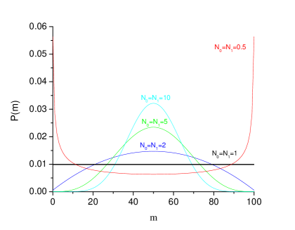
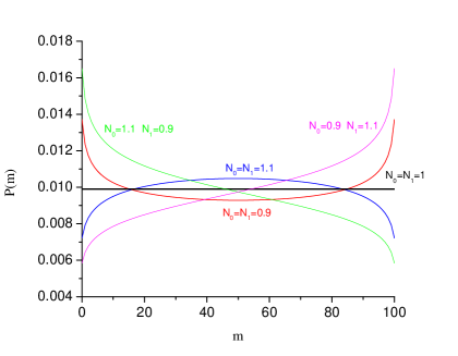
Figure 1: Asymptotic probability distribution for a network with $N=100$ nodes and several values of $N_{0}$ and $N_{1}$.

If $N$ is very large $\rho(m)$ peaks around $m_{0}$ and can be approximated by a Gaussian:

$$\rho(m)=\rho_{0}~{}\exp{-\left[\frac{(m-m_{0})^{2}}{2\Delta^{2}}\right]}.$$

with

$$\Delta=\left[\frac{NN_{0}N_{1}(N+N_{0}+N_{1})}{(N_{0}+N_{1})^{3}}\right]^{1/2}$$

and

$$\rho_{0}=\frac{1}{\sqrt{2\pi}\Delta}.$$

In terms of the continuous variables $x=m/N$, $n_{0}=N_{0}/N$ and $n_{1}=N_{1}/N$ we can also write

$$\rho(x)=\rho_{0}~{}\exp{-\left[\frac{(x-x_{0})^{2}}{2\delta^{2}}\right]}.$$

with

$$\delta=\left[\frac{n_{0}n_{1}(1+n_{0}+n_{1})}{N(n_{0}+n_{1})^{3}}\right]^{1/2}$$

$x_{0}=m_{0}/N$ and $\rho_{0}=1/\sqrt{2\pi}\delta$, showing that the width of the distribution goes to zero as $N$ goes to infinity, in agreement with the Hardy-Weinberg law.

VI Structured networks

For networks that are not fully connected the effect of the frozen nodes is amplified. To see this we note that the probability that a free node copies a frozen node is $P_{i}=(N_{0}+N_{1})/(N_{0}+N_{1}+k_{i})$ where $k_{i}$ is the degree of the node. For fully connected networks $k_{i}=N-1$ and $P_{i}\equiv P_{FC}$. For general networks an average value $P_{av}$ can be calculated by replacing $k_{i}$ by the average degree $k_{av}$. We can then define effective numbers of frozen nodes, $N_{0ef}$ and $N_{1ef}$, as being the values of $N_{0}$ and $N_{1}$ in $P_{FC}$ for which $P_{av}\equiv P_{FC}$. This leads to

$$N_{0ef}=fN_{0},\qquad\qquad N_{1ef}=fN_{1}$$ (9)

where $f=(N-1)/k_{av}$. Corrections involving higher moments can be obtained by integrating $P_{i}$ with the degree distribution and expanding around $k_{av}$.

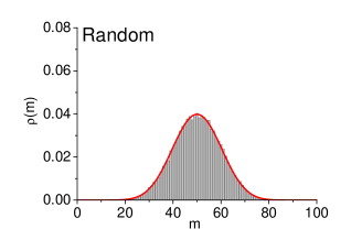
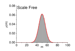
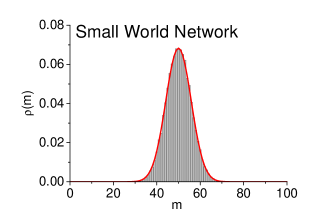
Figure 2: Equilibrium probability distribution for networks with different topologies. In all cases $N=100$, $N_{0}=N_{1}=5$, $t=10,000$, and the number of simulations is $50,000$. The theoretical (red) curve is drawn with effective numbers of frozen nodes $N_{0ef}=fN_{0}$ and $N_{1ef}=fN_{1}$: (a) random network $N_{0ef}=N_{1ef}=17$; (b) scale-free $N_{0ef}=N_{1ef}=82$; (c) regular 2-D lattice $N_{0ef}=N_{1ef}=140$; (d) small world network $N_{0ef}=N_{1ef}=140$.

Figure 2 shows examples of the equilibrium distribution for four different networks with $N=100$ and $N_{0}=N_{1}=5$. Panel (a) shows the result for a random network constructed by connecting any pair of nodes with probability $0.3$. In this case $k_{av}=29.7$ and $f=3.3$. The theoretical result was obtained with Eq. (5) with $N_{0ef}=N_{1ef}=17$. For a scale-free network (panel (b)) grown from an initial cluster of 6 nodes adding nodes with 3 connections each following the preferential attachment rule bararev , $f=99/6$ and the effective values of $N_{0}$ and $N_{1}$ are approximately 82. Panel (c) shows the probability distribution for a 2-D regular lattice with $10\times 10$ nodes connected to nearest neighbors for which $k_{a}v=3.6$ (the nodes near the border have less than 4 links) $f=99/3.6\approx 28$. Finally, panel (d) shows a small world version of the regular lattice bararev , where 30 connections were randomly re-allocated, creating shortcuts between otherwise distant nodes. These results show that the approximate re-scaling of frozen nodes (or, equivalently, the mutation rates) is accurate for many network topologies. Still, extreme cases such as a star network do present different distributions and this is confirmed by simulations.

VII Speciation and biodiversity

In the last sections we derived two important theoretical results: (a) the connection between the process of influence dynamics on networks and the Moran model; (b) the approximate equilibrium distribution for structured networks, obtained by re-scaling the number of frozen nodes. We will show now that these two results allow us to infer important properties about the genetic evolution of spatially extended populations.

It has been recently shown doursat2008 ; aguiar2009 that when mating is constrained by both spatial and genetic proximity between individuals, neutral evolution by drift alone might lead to speciation, i.e., to the spontaneous break up of the population into reproductively isolated clusters. Moreover, the patterns of abundance distributions generated by this mechanism are compatible with those observed in nature aguiar2009 .

Neutral theories of biodiversity have become rather sophisticated hubbell2001 , heating the neutralist-selectionist debate gavrilets2000 ; banavar2009 ; kopp2010 ; terSteege2010 ; etienne2010 . In what follows we discuss the process of neutral speciation promoted by spatial and genetic constraints, termed topopatric speciation, in the light of the theory developed above.

To make the analysis simpler we will restrict ourselves to the case of symmetric mutation rates, $\mu_{-}=\mu_{+}\equiv\mu$ or, equivalently, equal number of frozen nodes $N_{0}=N_{1}\equiv N_{z}$. In this case the connection between mutations and frozen nodes simplifies to

$$N_{z}=\displaystyle{\frac{2\mu(N-1)}{1-2\mu}}.$$ (10)

Let $P_{id}$ be the probability that two individuals picked at random in the population have identical genes at equilibrium. This is given by the sum of the probabilities that their alleles are are both $A_{1}$ or both $A_{0}$:

$$\begin{array}[]{ll}P_{id}&=\sum_{m=0}^{N}\rho(m)\left[\frac{m}{N}\frac{m-1}{N-1}+\frac{N-m}{N}\frac{N-m-1}{N-1}\right]\\ \\ &=1+\frac{2}{N(N-1)}\left[\sigma^{2}+\langle m\rangle^{2}-N\langle m\rangle\right].\end{array}$$

Using equations (7), (8) and (10) we obtain

$$P_{id}=\frac{1+N_{z}}{1+2N_{z}}=\frac{1+2\mu(N-2)}{1+2\mu(2N-3)}.$$ (11)

The probability that the two individuals are different, which is the heterozigosity, is

$$P_{ht}=1-P_{id}=\frac{2\mu(N-1)}{1+2\mu(2N-3)}\approx\frac{2\mu N}{1+4\mu N}$$ (12)

where the approximation holds for $N>>1$.

Consider now a population in equilibrium where the $N$ individuals have $B$ independent genes higgs1991 ; zhang1997 ; jensen2002 ; jain2007 ; doursat2008 ; aguiar2009 . The average genetic distance between two individuals is

$$\langle d\,\rangle=BP_{ht}\approx\frac{B}{2}\left(\frac{4\mu N}{1+4\mu N}\right).$$ (13)

This expression provides a connection between the size of the population and the average genetic distance between individuals, which is a measure of diversity within the population. Two interesting relations can be derived from this equation: first, for given $B$ and $\mu$ we can calculate the size $N_{G}$ that corresponds to a particular average genetic distance $\langle d\,\rangle=G$:

$$N_{G}=\frac{G}{2\mu(B-2G)}.$$ (14)

Second, for given $N$ and $B$ we calculate the mutation rate $\mu_{G}$ that corresponds to $\langle d\,\rangle=G$:

$$\mu_{G}=\frac{G}{2N(B-2G)}.$$ (15)

Notice that $N_{G}\mu=N\mu_{G}$.

When mating in panmictic populations is constrained by genetic proximity between individuals, so that pairs whose genetic distance is larger than $G$ are incompatible, the distribution of genetic distances stays very close to $\langle d\,\rangle=G$, as if the genome had an effective size $B_{ef}=2G$. On the other hand, if mating is constrained by spatial proximity, the effective mutation rate tends to increase. Indeed, spatial restriction in mating corresponds to influence processes on networks constructed over regular lattices, which amplifies the effect of frozen nodes and, therefore, of mutations.

Consider a square lattice with $L^{2}$ nodes and periodic boundary conditions where each node is connected only to neighbors which are within a distance $S$ from itself (measured in units of lattice spacing). Let $N$ be the number of individuals in the population, so that the density is $\rho=N/L^{2}$. The area where an individual can look for a mate, its ‘mating neighborhood’, is approximately $\pi S^{2}$, which is also the average degree $k_{av}$ of the network.

According to our discussion in section VI, this can be modeled as fully connected network with effective number of frozen nodes

$$N_{ef}=fN_{z}=\frac{N-1}{k_{av}}\,N_{z}\approx\frac{N}{\pi S^{2}}N_{z}.$$ (16)

The corresponding effective mutation rate is obtained from (10)

$$N_{ef}=\frac{2\mu_{ef}(N-1)}{1-2\mu_{ef}}$$

which gives

$$\mu_{ef}=\frac{f}{1+2\mu(f-1)}\mu\approx\frac{\mu f}{1+2\mu f}.$$ (17)

Note that $\mu_{ef}\rightarrow 1/2$ if $\mu f>>1$.

When mating between individuals is constrained by their spatial distance, as measured by the parameter $S$, the effective mutation rate (17) can be dramatically enhanced with respect to a panmictic population. This, in turn, increases the average genetic distance between individuals, which approaches $B/2$ for large populations and fixed $k_{av}$ (corresponding to large values of $N_{z}$). The distribution of genetic distances approaches a broad symmetric distribution.

On the other hand, if mating is constrained only by the genetic distance between individuals, the distribution of genetic distances shrinks to about $G$. This corresponds to an effective shrink in genome size from $B$ to $2G$.

When both spatial and genetic restrictions are present, as in aguiar2009 , the population feels a large effective mutation rate, tending to spread out the genome distribution. On the other hand, the individuals are compelled by the mating condition to stay genetically close to each other. The only stable outcome of these opposing forces is the formation of local groups where $\langle d\,\rangle\leq G$ within the group but $\langle d\,\rangle>G$ among groups. This characterizes the groups as reproductively isolated from each other and, therefore, as separate species.

The average number of individuals in each group is given approximately by $N_{G}$ (14), which is usually much smaller than $N$. This also implies that the individuals within groups are highly connected to each other, so that $f\approx 1$ and $\mu_{ef}\approx\mu$, restoring the equilibrium of the system.

The conditions for speciation can be estimated as follows. When $S$ is very large, the effect of the genetic mating restriction is to reduce the effective size of the genome, $B_{ef}$, from $B$ to $2G$, so that, from equation (13), $\langle d\,\rangle$ is at most $G$. As $S$ is reduced, the effective mutation rate increases and new genes are incorporated into the effective genome, increasing the average genetic distance between individuals. When $\langle d\,\rangle$ becomes larger than about $2G$ the population can no longer hold itself together and splits. This has been confirmed by numerical simulations. We write

$$B_{ef}=2G+(B-2G){\cal P}$$ (18)

where ${\cal P}$ is the probability that a new gene is fixed into the effective genome.

${\cal P}$ goes to zero for large values of $S$ and reaches one for small $S$. It must depend only on the mutation rate $\mu$, genome length $B$ and the size of the local mating population $N_{S}\equiv\pi S^{2}\rho=\pi S^{2}N/L^{2}$. This local mating population has to be at least 2, otherwise mating is not possible. More generally, if the minimum number of potential mates for reproduction is $P$ we can define the minimum $S$ by $\pi S_{min}^{2}\rho=P$, or

$$S_{min}=L\sqrt{P/\pi N}.$$ (19)

${\cal P}$ must be small if the local mating population is large. On the other hand, it must increase with the mutation rate and size of the genome. We may therefore write the ansatz

$${\cal P}=\exp{\left\{-c\left[\frac{\pi(S-S_{min})^{2}N/L^{2})}{B\mu}\right]^{2}\right\}}$$

or

$${\cal P}=\exp{\left\{-\frac{\pi^{2}(S-S_{min})^{4}N^{2}}{\gamma^{4}L^{4}B^{2}\mu^{2}}\right\}}.$$ (20)

where the constant of proportionality $c$ is rewritten by as $\gamma^{-4}$ for convenience. The exponential dependence of ${\cal P}$ on the square of $N_{S}/B\mu$ is suggested by numerical simulations.

Figure 3: Parameter region where speciation is possible according with equation (22). In this example $N=2000$, $\mu=0.001$, $B=125$, $L=128$ and $P=8$ ($S_{min}=4.6$) and $\gamma=6.6$ (see aguiar2009 ).

The condition for speciation is

$$\langle d\,\rangle=\frac{B_{ef}}{2}\left(\frac{4\mu_{ef}N}{1+4\mu_{ef}N}\right)\gtrsim 2G.$$

Since the $\mu N$ is usually of order 1 in most simulations, and $\mu_{ef}>>\mu$, the factor $4\mu_{ef}N/(1+4\mu_{ef}N)$ can be safely approximated by 1. Using equations (18) and (20) we obtain

$$\frac{\pi^{2}(S-S_{min})^{4}N^{2}}{\gamma^{4}L^{4}\mu^{2}B^{2}}\lesssim\log{\left(\frac{B-2G}{2G}\right)}$$

or

$$S\lesssim S_{min}+\gamma L\sqrt{\frac{B\mu}{N\pi}}\left[\log{\left(\frac{B-2G}{2G}\right)}\right]^{1/4}\equiv S_{c}(G).$$ (21)

Inverting this equation we obtain

$$G\lesssim\frac{B/2}{1+\exp{\left(\frac{\pi^{2}N^{2}(S-S_{min})^{4}}{\gamma^{4}\mu^{2}B^{2}L^{4}}\right)}}\equiv G_{c}(S)$$ (22)

which gives the minimum value of $G$ for a given $S$.

Equation (21) gives the maximum size of the mating neighborhood for which speciation is possible. This analytical result describes the dependence of speciation on 6 model parameters: $B$, $G$, $\mu$, $P$, $L$ and $N$. It provides a very good quantitative estimate for the parameter region where speciation is possible, as illustrated in figure 3. The result also incorporates cutoffs at $G=B/4$ and at $S_{min}$, which are in agreement with numerical simulations aguiar2009 . Furthermore it also gives the scaling dependence of $S_{c}$ on these various parameters. In particular, it predicts speciation at large values of $S$ if $B$ is sufficiently large. This corroborates the results in higgs1991 ; higgs1992 but shows that such space-independent speciation occurs only for very large values of $B$, since $S$ increases with $B^{1/2}$.

Our analytical result constitute an important addition to the simulations presented in aguiar2009 and contribute to the understanding of the significant role of drift in speciation coyne ; aguiar2009 ; doursat2008 ; hubbell2001 ; higgs1991 ; kopp2010 ; terSteege2010 . Equation (21) identifies the combination of parameters that makes this possible. For example, low mutation rates, that hinder speciation, can be compensated by a large number of participating genes or by low population density.

VIII Conclusions

The process of speciation underlies the creation of the tree of life. Fossil records and molecular analysis allow the construction of detailed phylogenetic trees linking species to their ancestors, identifying the branching points of speciation. The way speciation occurred in each case, however, is rarely known with certainty and several mechanisms have been considered. A recently proposed mechanism of speciation (aguiar2009, ) demonstrated that a spatially extended population can break up spontaneously into species when subjected to mutations and to spatial and genetic mating restrictions, even in the absence of natural selection. Numerical simulations have shown that this mechanism, termed topopatry, occurs for a restricted range of parameters, that include population size $N$, mutation rate $\mu$ and the parameters $S$ and $G$ controlling the spatial and genetic mating restrictions.

In this paper we have introduced a mapping of genetic dynamics in an evolving population onto the dynamics of influence on a network, and used this mapping to analytically study the process of topopatric speciation. This mapping gives, to our knowledge, the first complete solution of the Moran model, providing an elegant representation of the complete set of eigenvectors of the problem.

We have shown that, while fully connected networks correspond to panmictic populations, certain structured networks can be mapped into dynamic spatially extended populations. Moreover, the mapping shows that limiting mating to a fraction of the total population by network connections increases the effective mutation rate as compared to the panmictic case, and increases the genetic diversity of the population. By extending the model from one to multiple independent biallelic genes, we have shown that a genetic restriction on mating decreases the effective size of the genome, decreasing diversity. These opposing forces are resolved not by compromise but by pattern formation, breaking up the population into multiple species. This process, and its dependence on the most relevant characteristics of the population, is accurately described by equation (22). This equation provides a new and important tool to understand neutral speciation, revealing explicitly the relationships among the parameters involved in the process, and the interplay of genetic processes whose opposition leads to spontaneous speciation.

ACKNOWLEDGMENTS

It is a pleasure to thank Elizabeth M. Baptestini for helpful comments. MAMA acknowledges financial support from CNPq and FAPESP.

References

- (1) W.J. Ewens Mathematical Population Genetics I. Theoretical Introduction Series: Biomathematics, Vol. 9 (New York: Springer Verlag, 1979).
- (2) C. Cannings, Adv. Appl. Prob. 6 260 (1974).
- (3) P.A.P. Moran, Proc. Cam. Phil. Soc. 54 60 (1958).
- (4) J. Wakeley Coalescent theory (Roberts & Company Publishers, 2009).
- (5) G.A. Watterson, The Annals of Mathematical Statistics 32, 716 (1961).
- (6) K. Gladstien, Siam J. Appl. Math 34 630 (1978).
- (7) J.H. Gillespie. Population Genetics: A concise guide (The Johns Hopkins University Press, 2004).
- (8) M.A.M. de Aguiar, I.R. Epstein and Y. Bar-Yam, Phys. Rev. E 72 067102 (2005).
- (9) D.D. Chinellato, M.A.M. de Aguiar, I.R. Epstein, D. Braha and Y. Bar-Yam, arXiv:0705.4607v2 [nlin.SI]
- (10) S. Wright, Genetics 28 114 (1943).
- (11) M.A.M. de Aguiar, M. Baranger, E.M. Baptestini, L. Kaufman, and Y. Bar-Yam, Nature 460 384 (2009).
- (12) M.L. Rosenzweig, Species diversity in space and time, (Cambridge University Press, 1995)
- (13) R. Albert and A.-L. Barabási, Rev. Mod. Phys. 74, 47 (2002).
- (14) G.A. Hoelzer, R. Drewes, J. Meier and R. Doursat, PLoS Comput. Biol. 4 e1000126 (2008).
- (15) S.P. Hubbell, The Unified Neutral Theory of Biodiversity and Biogeography, (Princeton University Press, New Jersey, 2001).
- (16) M. Kopp, BioEssays 32 564 (2010).
- (17) H. Ter Steege, Biotropica 42 631 (2010)
- (18) S. Gavrilets, Li Hai and M.D. Vose, Evolution 54 1126 (2000).
- (19) R.S. Etienne and B. Haegeman, Theor. Ecol. 4 87 (2011).
- (20) J.R. Banavar and A. Maritan, Nature 460 334 (2009).
- (21) P.G. Higgs and B.Derrida, J. Phys. A. 24, L985 (1991).
- (22) P.G. Higgs and B.Derrida, J. Mol. Evol., 35, 454 (1992).
- (23) Yi-Cheng Zhang, Phys. Rev. E 55, R3817 (1997).
- (24) M. Hall, K. Christensen, S. A. di Collobiano, and H. J. Jensen, Phys. Rev. E 66, 011904 (2002).
- (25) K. Jain, Phys. Rev. E 76, 031922 (2007).
- (26) J.A. Coyne and H.A. Orr Speciation, (Sinauer Associates, MA, 2004).