Anomalous temperature dependence of the order parameter of a superconductor with weakly correlated impurities

I. A. Fomin
P. L. Kapitza Institute for Physical Problems,
Kosygina 2, 119334 Moscow, Russia;
Moscow Institute of Physics and Technology,
Dolgoprudny, Mosow region
Abstract

It is shown that weak correlations between pair-breaking impurities in superconductors influence the temperature dependence of the order parameter within the Ginzburg and Landau region if correlation radius of impurities $R$ is greater than the coherence length of the superconductor $\xi_{0}$. Dependence of a square of the average order parameter on the temperature difference $T_{c}-T$ changes its slope in a region $\xi_{0}\sqrt{T_{c}/(T_{c}-T)}\sim R$. Influence of correlations of impurities on other thermodynamic properties of superconductors is discussed.

Impurities make the condensate of Cooper pairs spatially nonuniform. Manifestation of this non-uniformity is particularly strong in unconventional superconductors and in conventional superconductors with magnetic impurities. In a vicinity of the transition temperature $T_{c}$ free energy of such superconductor can be written as Ginzburg and Landau functional with coefficients, which are random functions of coordinate. For a scalar order parameter $\Psi(\textbf{r})$

$$\emph{F}_{s}\{\Psi(\textbf{r})\}=\emph{F}_{n}+\int\{a(\textbf{r})|\Psi(\textbf{r})|^{2}+\frac{1}{2}b(\textbf{r})|\Psi(\textbf{r})|^{4}+c(\textbf{r})|\nabla\Psi(\textbf{r})|^{2}\}d^{3}r.$$ (1)1

According to the analysis of Larkin and Ovchinnikov [1] the most strong effect on the average order parameter have fluctuations of the coefficient $a(\textbf{r})$ i.e. fluctuations of the local transition temperature $T_{c}(\textbf{r})$: $a(\textbf{r})=\alpha(T-T_{c}(\textbf{r}))$. Because of these fluctuations the temperature dependence of the average order parameter $\langle\Psi\rangle$ deviates from the linear dependence $\langle\Psi\rangle^{2}\sim(T_{c}-T)/T_{c}$ characteristic of the uniform superconductor and becomes singular in a narrow interval below the superfluid transition temperature $(T_{c}-T)/T_{c}\sim(\xi_{0}/l)^{4}(1/(n\xi_{0})^{2})$, where $l$ is the mean free path and $n$ - the density of impurities. The linear dependence is preserved outside of this region. This result is obtained under assumption that impurities are not correlated. It has been shown recently, that correlations with a radius $R$ which is greater than $\xi_{0}$ strongly affect suppression of $T_{c}$ by impurities [2, 3]. Such situation is realized for the superfluid 3He in aerogel. Experimental data for thermodynamic properties of superfluid 3He in aerogel, such as the square of the Leggett frequency $\Omega_{L}^{2}$ and ρssubscriptπœŒπ‘ \rho_{s} [4, 5] deviate from the linear dependence on $T_{c}-T$ in a much wider interval of temperatures than that, estimated on a basis of Ref.[1]. The observed dependence of these quantities bends upward when $T_{c}-T$ increases. The aim of this paper is to show that this anomaly can be interpreted as the effect of correlations among the impurities. The effect of correlations is general in a sense, that presence and a character of deviations do not depend on a particular form of the order parameter. For demonstration of the effect the simplest example of a superconductor with the scalar order parameter $\Psi(\textbf{r})$ will be considered.

Let us follow the argument of Ref.[1] with the modifications required by the presence of correlations. Free energy (1) can be rewritten in terms of the dimensionless order parameter $\psi(\textbf{r})=\Psi(\textbf{r})/\Psi_{0}$, where $\Psi_{0}$ is the absolute value of the order parameter for pure superconductor at $T=0$ obtained by extrapolation of linear dependence of $|\Psi|^{2}$ on $(T_{c0}-T)$ from the transition temperature of the pure superconductor $T_{c0}$:

Fs​{Οˆβ€‹(r)}=Fn+Tc​0​Δ​c0β€‹βˆ«{[Ο„βˆ’Ξ·β€‹(r)]​|Οˆβ€‹(r)|2+12​|Οˆβ€‹(r)|4+ΞΎs2​|βˆ‡Οˆβ€‹(r)|2}​d3​r.subscriptFπ‘ πœ“rsubscriptF𝑛subscript𝑇𝑐0Ξ”subscript𝑐0delimited-[]πœπœ‚rsuperscriptπœ“r212superscriptπœ“r4superscriptsubscriptπœ‰π‘ 2superscriptβˆ‡πœ“r2superscript𝑑3π‘Ÿ\emph{F}_{s}\{\psi(\textbf{r})\}=\emph{F}_{n}+T_{c0}\Delta c_{0}\int\{[\tau-\eta(\textbf{r})]|\psi(\textbf{r})|^{2}+\frac{1}{2}|\psi(\textbf{r})|^{4}+\xi_{s}^{2}|\nabla\psi(\textbf{r})|^{2}\}d^{3}r. (2)2

Other notations here are: $\Delta c_{0}$ – the specific heat jump in the pure superconductor, $\tau=(T-T_{c1})/T_{c0}$, $T_{c1}=\langle T_{c}(\textbf{r})\rangle$, so that the relative fluctuation of local transition temperature $\eta(\textbf{r})=(T_{c}(\textbf{r})-T_{c1})/T_{c0}$, it vanishes after averaging. The elasticity coefficient ΞΎs2=7​΢​(3)12​ξ02superscriptsubscriptπœ‰π‘ 27𝜁312superscriptsubscriptπœ‰02\xi_{s}^{2}=\frac{7\zeta(3)}{12}\xi_{0}^{2} in the BCS theory. In these notations Ginzburg and Landau equation reads as:

[Ο„βˆ’Ξ·β€‹(r)]β€‹Οˆ+Οˆβ€‹|ψ|2βˆ’ΞΎs2β€‹Ξ”β€‹Οˆ=0delimited-[]πœπœ‚rπœ“πœ“superscriptπœ“2superscriptsubscriptπœ‰π‘ 2Ξ”πœ“0[\tau-\eta(\textbf{r})]\psi+\psi|\psi|^{2}-\xi_{s}^{2}\Delta\psi=0 (3)3

At $T<T_{c}$ the long-range order is established, characterized by the average order parameter $\langle\psi\rangle$. The angular brackets denote averaging over ensemble of impurities. Solution of Eq. (3) can be sought in a form $\psi(\bf{r})=\langle\psi\rangle(1+\chi({\bf r}))$. When $\eta({\bf r})$ is small $\chi({\bf r})$ is small too, except for the mentioned above temperature region close to $T_{c}$, where $\langle\chi({\bf r})\chi({\bf r})\rangle$ diverges. Averaging Eq.(3) over ensemble of impurities renders expression for $\langle\psi\rangle^{2}$ in terms of the average products $\langle\eta\chi\rangle$ and $\langle\chi\chi\rangle$:

$$\langle\psi\rangle^{2}=\frac{\langle\eta\chi\rangle-\tau}{1+3\langle\chi\chi\rangle}$$ (4)4

The fluctuating part $\chi(\bf{r})$ can be found from the linearized equation (2):

(Ο„βˆ’Ξ·β€‹(𝐫)+3β€‹βŸ¨ΟˆβŸ©2)β€‹Ο‡βˆ’ΞΎs2​Δ​χ=η​(𝐫)βˆ’βŸ¨Ξ·β€‹Ο‡βŸ©.πœπœ‚π«3superscriptdelimited-βŸ¨βŸ©πœ“2πœ’superscriptsubscriptπœ‰π‘ 2Ξ”πœ’πœ‚π«delimited-βŸ¨βŸ©πœ‚πœ’(\tau-\eta({\bf r})+3\langle\psi\rangle^{2})\chi-\xi_{s}^{2}\Delta\chi=\eta({\bf r})-\langle\eta\chi\rangle. (5)5

Its solution can be formally written in terms of the Green function $G({\bf r},{\bf r^{\prime}})$:

$$\chi({\bf r})=\int G({\bf r},{\bf r^{\prime}})(\eta({\bf r^{\prime}})-\langle\eta\chi\rangle)d^{3}r^{\prime}.$$ (6)6

Re-writing this solution in the momentum representation we can find the averages, entering Eq. (4):

$$\langle\eta(\textbf{r})\chi(\textbf{r})\rangle=\int\langle\eta(\textbf{-k})G({\bf k},{\bf k^{\prime}})\eta({\bf k^{\prime}})\rangle\frac{d^{3}k}{(2\pi)^{3}}\frac{d^{3}k^{\prime}}{(2\pi)^{3}}\left[1+\int\langle\eta({\bf-k})G(\textbf{k},0)\rangle\frac{d^{3}k}{(2\pi)^{3}}\right]^{-1}$$ (7)7

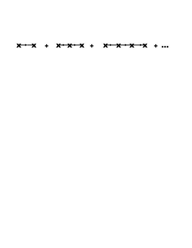
The average in the numerator can be found by term-by-term averaging of the diagrammatic series Fig.1.

Refer to caption
Figure 1: Β 

To every arrow here corresponds the unperturbed Green function G0​(𝐀,𝐀′)=(2​π)3​δ​(π€βˆ’π€β€²)​[Ο„+3β€‹βŸ¨ΟˆβŸ©2+ΞΎs2​k2]βˆ’1subscript𝐺0𝐀superscript𝐀′superscript2πœ‹3𝛿𝐀superscript𝐀′superscriptdelimited-[]𝜏3superscriptdelimited-βŸ¨βŸ©πœ“2superscriptsubscriptπœ‰π‘ 2superscriptπ‘˜21G_{0}({\bf k},{\bf k^{\prime}})=(2\pi)^{3}\delta({\bf k}-{\bf k^{\prime}})[\tau+3\langle\psi\rangle^{2}+\xi_{s}^{2}k^{2}]^{-1} and to a cross $\eta(\textbf{k}_{1}-\textbf{k}_{2})$, $\textbf{k}_{1}$ is the in-coming and $\textbf{k}_{2}$ – the out-going momenta. Comparison of the averaged diagrammatic series Fig.1 with that for the average Green function relates $\langle\eta G\eta\rangle$ to $\langle G\rangle$:

$$\langle\eta G\eta\rangle=G_{0}^{-1}[\langle G\rangle G_{0}^{-1}-1],$$ (8)8

which in its turn can be expressed in terms of the self-energy $\Sigma(\textbf{k},\tau)$:

⟨G​(k)⟩=[Ο„+3β€‹βŸ¨ΟˆβŸ©2βˆ’Ξ£β€‹(k,Ο„)+ΞΎs2​k2]βˆ’1delimited-⟨⟩𝐺ksuperscriptdelimited-[]𝜏3superscriptdelimited-βŸ¨βŸ©πœ“2Ξ£k𝜏superscriptsubscriptπœ‰π‘ 2superscriptπ‘˜21\langle G(\textbf{k})\rangle=[\tau+3\langle\psi\rangle^{2}-\Sigma(\textbf{k},\tau)+\xi_{s}^{2}k^{2}]^{-1} (9)9

Using analogous argument for evaluation of $\langle\eta G\rangle$ we find eventually that

$$\langle\chi\eta\rangle=\Sigma(0,\tau).$$ (10)10

In a principal order on the perturbation $\eta(\textbf{r})$

Σ​(0,Ο„)=βˆ«βŸ¨Ξ·β€‹(-k1)​η​(k1)βŸ©Ο„+3β€‹βŸ¨ΟˆβŸ©2βˆ’Ξ£β€‹(k1,Ο„)+ΞΎs2​k12​d3​k1(2​π)3.Ξ£0𝜏delimited-βŸ¨βŸ©πœ‚subscript-k1πœ‚subscriptk1𝜏3superscriptdelimited-βŸ¨βŸ©πœ“2Ξ£subscriptk1𝜏superscriptsubscriptπœ‰π‘ 2superscriptsubscriptπ‘˜12superscript𝑑3subscriptπ‘˜1superscript2πœ‹3\Sigma(0,\tau)=\int\frac{\langle\eta(\textbf{-k}_{1})\eta(\textbf{k}_{1})\rangle}{\tau+3\langle\psi\rangle^{2}-\Sigma(\textbf{k}_{1},\tau)+\xi_{s}^{2}k_{1}^{2}}\frac{d^{3}k_{1}}{(2\pi)^{3}}. (11)11

Of practical interest is a situation when $\eta(\textbf{r})=\sum_{a}\eta^{(1)}(\textbf{r}-\textbf{r}_{a})$, where $\eta^{(1)}(\textbf{r}-\textbf{r}_{a})$ is a contribution of individual impurity situated at the position $\textbf{r}_{a}$. In that case the correlation function $\langle\eta(\textbf{-k})\eta(\textbf{k})\rangle=n|\eta^{(1)}(\textbf{k})|^{2}S(\textbf{k})$, where $S(\textbf{k})=\langle\sum_{b}\exp[i\textbf{k}(\textbf{r}_{b}-\textbf{r}_{a})]\rangle$ is the structure factor. For non-correlated impurities only one term with $\textbf{r}_{b}=\textbf{r}_{a}$ contributes to the sum. Effect of correlations is contained in $\bar{S}(\textbf{k})=S(\textbf{k})-1$, which is Fourier transform of the correlation function in the coordinate space $v(\textbf{r})$. When impurities are correlated on a distance $\sim R$ the $\bar{S}(\textbf{k})$ is enhanced for $k\sim 1/R$. For estimation of the effect of correlations a model expression (”$\delta$-model”[3]): $\bar{S}(\textbf{k})=2\pi^{2}R^{2}nv(0)\delta(k-1/R)$ can be used. In particular, one can show that corrections to the principal expression for $\Sigma(0,\tau)$, given by Eq.(11) contain extra factor $R^{2}/\xi_{0}l\equiv\varepsilon$. In what follows we assume, that $\varepsilon\ll 1$ and treat effect of correlation as a perturbation. In a principal order on $\varepsilon$ in the denominator of the integrand in Eq. (11) we can set $\langle\psi\rangle^{2}=\Sigma(0,\tau)-\tau$ and take $\Sigma(\textbf{k},\tau)\approx\Sigma(0,\tau)$. Then Eq. (11) determines a function $\Sigma(0,\tau)$. In this equation a combination $u=\Sigma(0,\tau)-\tau$ is taken as a new variable. In the expression (11) for $\Sigma(0,\tau)$ we separate part which is finite at $u=0$. As was discussed before [2, 3], it determines the second order correction to the shift of $T_{c}$. The new transition temperature $T_{c2}$ is then Tc​2=Tc​1+Tc​0β€‹βˆ«n​|Ξ·(1)​(k1)|2​S​(k1)ΞΎs2​k12​d3​k1(2​π)3subscript𝑇𝑐2subscript𝑇𝑐1subscript𝑇𝑐0𝑛superscriptsuperscriptπœ‚1subscriptk12𝑆subscriptk1superscriptsubscriptπœ‰π‘ 2superscriptsubscriptπ‘˜12superscript𝑑3subscriptπ‘˜1superscript2πœ‹3T_{c2}=T_{c1}+T_{c0}\int\frac{n|\eta^{(1)}(\textbf{k}_{1})|^{2}S(\textbf{k}_{1})}{\xi_{s}^{2}k_{1}^{2}}\frac{d^{3}k_{1}}{(2\pi)^{3}}. It is convenient to introduce a variable $t$, which counts temperature from $T_{c2}$: $t=(T-T_{c2})/T_{c0}$. In these notations Eq.(11) renders relation between $u$ and $t$:

u​[1+2β€‹βˆ«n​|Ξ·(1)​(k1)|2​S​(k1)ΞΎs2​k12​[2​u+ΞΎs2​k12]​d3​k1(2​π)3]=βˆ’t.𝑒delimited-[]12𝑛superscriptsuperscriptπœ‚1subscriptk12𝑆subscriptk1superscriptsubscriptπœ‰π‘ 2superscriptsubscriptπ‘˜12delimited-[]2𝑒superscriptsubscriptπœ‰π‘ 2superscriptsubscriptπ‘˜12superscript𝑑3subscriptπ‘˜1superscript2πœ‹3𝑑u\left[1+2\int\frac{n|\eta^{(1)}(\textbf{k}_{1})|^{2}S(\textbf{k}_{1})}{\xi_{s}^{2}k_{1}^{2}[2u+\xi_{s}^{2}k_{1}^{2}]}\frac{d^{3}k_{1}}{(2\pi)^{3}}\right]=-t. (12)12

In terms of $u$ $\langle\psi\rangle^{2}=u/(1+3\langle\chi\chi\rangle)$. When $S(\textbf{k}_{1})$ is strongly peaked at $k_{1}\sim 1/R$ the dependence of $u$ on $t$ changes its slope in a region u∼(ΞΎs/R)2similar-to𝑒superscriptsubscriptπœ‰π‘ π‘…2u\sim(\xi_{s}/R)^{2}, i.e. when $\xi(T)\sim R$ and $\xi(T)$ is defined as $\xi_{0}/\sqrt{u}$. At u≫(ΞΎs/R)2much-greater-than𝑒superscriptsubscriptπœ‰π‘ π‘…2u\gg(\xi_{s}/R)^{2} asymptotically $u\approx(T_{c1}-T)/T_{c0}$, i.e. it depends linearly on a distance from the average transition temperature $T_{c1}$. In the opposite limit uβ‰ͺ(ΞΎs/R)2much-less-than𝑒superscriptsubscriptπœ‰π‘ π‘…2u\ll(\xi_{s}/R)^{2} u is linear in $t=(T_{c2}-T)/T_{c0}$, with a different slope. The relative change of the slope is on the order of $\varepsilon^{2}$. Using for $\bar{S}(\textbf{k})$ the $\delta$-model we have:

u=t1+2​n2​|Ξ·(1)​(0)|2​v​(0)​(R/ΞΎs)4.𝑒𝑑12superscript𝑛2superscriptsuperscriptπœ‚102𝑣0superscript𝑅subscriptπœ‰π‘ 4u=\frac{t}{1+2n^{2}|\eta^{(1)}(0)|^{2}v(0)(R/\xi_{s})^{4}}. (13)13

If impurities, like aerogel, have a tendency to form clusters, $v(0)>0$ and the slope of $u(t)$ at uβ‰ͺ(ΞΎs/R)2much-less-than𝑒superscriptsubscriptπœ‰π‘ π‘…2u\ll(\xi_{s}/R)^{2} is smaller than at u≫(ΞΎs/R)2much-greater-than𝑒superscriptsubscriptπœ‰π‘ π‘…2u\gg(\xi_{s}/R)^{2}, so the $u(t)$ bends upward. Together with $u(t)$ changes its slope $\langle\psi\rangle^{2}(t)=u/(1+3\langle\chi\chi\rangle)$. The average $\langle\chi\chi\rangle$ in the denominator is on the order of $\varepsilon^{2}$:

βŸ¨Ο‡β€‹Ο‡βŸ©=∫n​|Ξ·(1)​(k)|2​S​(k)[2​u+ΞΎs2​k2]2​d3​k(2​π)3.delimited-βŸ¨βŸ©πœ’πœ’π‘›superscriptsuperscriptπœ‚1k2𝑆ksuperscriptdelimited-[]2𝑒superscriptsubscriptπœ‰π‘ 2superscriptπ‘˜22superscript𝑑3π‘˜superscript2πœ‹3\langle\chi\chi\rangle=\int\frac{n|\eta^{(1)}(\textbf{k})|^{2}S(\textbf{k})}{[2u+\xi_{s}^{2}k^{2}]^{2}}\frac{d^{3}k}{(2\pi)^{3}}. (14)14

This correction does not influence asymptotic of the dependence of $\langle\psi\rangle^{2}$ on $t$ at u≫(ΞΎs/R)2much-greater-than𝑒superscriptsubscriptπœ‰π‘ π‘…2u\gg(\xi_{s}/R)^{2}, but at uβ‰ͺ(ΞΎs/R)2much-less-than𝑒superscriptsubscriptπœ‰π‘ π‘…2u\ll(\xi_{s}/R)^{2} it increases the change of the slope. Due to this correction physical quantities, which depend on averages of different powers of the order parameter will have different changes of the slope. E.g. the NMR frequencies are proportional to $\langle\psi^{2}\rangle=\langle\psi\rangle^{2}(1+\langle\chi\chi\rangle)\simeq u/(1+2\langle\chi\chi\rangle)$. For the model $\bar{S}\sim\delta(k-1/R)$ at uβ‰ͺ(ΞΎs/R)2much-less-than𝑒superscriptsubscriptπœ‰π‘ π‘…2u\ll(\xi_{s}/R)^{2}:

⟨ψ2⟩=t1+4​n2​|Ξ·(1)​(0)|2​v​(0)​(R/ΞΎs)4.delimited-⟨⟩superscriptπœ“2𝑑14superscript𝑛2superscriptsuperscriptπœ‚102𝑣0superscript𝑅subscriptπœ‰π‘ 4\langle\psi^{2}\rangle=\frac{t}{1+4n^{2}|\eta^{(1)}(0)|^{2}v(0)(R/\xi_{s})^{4}}. (15)15

Further thermodynamic properties can be found as derivatives of the average free energy over $T$. Using the expression $\emph{F}_{s}-\emph{F}_{n}=-\frac{T_{c0}\Delta c_{0}}{2}\langle\int|\psi|^{4}d^{3}r\rangle$ and relation $\langle|\psi|^{4}\rangle=\langle\psi\rangle^{4}(1+6\langle\chi\chi\rangle)$ we arrive at:

$$\emph{F}_{s}-\emph{F}_{n}=-\frac{T_{c0}\Delta C_{0}}{2}u^{2},$$ (16)16

i.e. a gain of the free energy is proportional to $u^{2}$ and not to $t^{2}$. The specific heat jump, following from Eq. (16) is:

$$\Delta C_{i}=\Delta C_{0}T_{c0}T_{c2}\left(\frac{du}{dt}\right)^{2}_{T\to T_{c2}}.$$ (17)17

For the $\delta$-model Δ​Ci=Δ​C0​Tc​2Tc​0​(1+2​n2​|Ξ·(1)​(0)|2​v​(0)​(R/ΞΎs)4)βˆ’2Ξ”subscript𝐢𝑖Δsubscript𝐢0subscript𝑇𝑐2subscript𝑇𝑐0superscript12superscript𝑛2superscriptsuperscriptπœ‚102𝑣0superscript𝑅subscriptπœ‰π‘ 42\Delta C_{i}=\Delta C_{0}\frac{T_{c2}}{T_{c0}}(1+2n^{2}|\eta^{(1)}(0)|^{2}v(0)(R/\xi_{s})^{4})^{-2}. There is extra suppression of the jump due to correlations.

So, we conclude, that the anomaly of temperature dependence of thermodynamic properties of superfluid 3He in aerogel is qualitatively the same as that found in the considered example of a superconductor with a one-component order parameter and correlated impurities. The quantitative comparison of the obtained results with the data for 3He would not have sense, because superfluid 3He has a multi component order parameter. This opens a possibility for correlated impurities to interact with several different modes of fluctuations of the order parameter. For a quantitative description of the anomaly all of these modes have to be taken into account. Nevertheless a qualitative estimation of the correlation radius based on the relation $\xi(T)\approx R$ at a temperature of a change of the slope is close to other estimations.

Because of its universal character the anomaly can occur in superconductors with different order parameters and can be considered as an indication that impurities are correlated and correlation radius is greater than $\xi_{0}$. A distance from $T_{c}$ at which dependence of $\langle\psi\rangle^{2}$ on $T_{c}-T$ changes its slope renders estimation of the correlation radius.

I thank E.V. Surovtsev for useful discussions. This work was supported in part by RFBR grant # 09-02-12131 ofi-m.

References

  • [1] A.i. Larkin and Yu.N. Ovchinnikov, ZhETF 61, 1221 (1971), [Sov. Phys. JETP 34, 651 (1972)].
  • [2] I.A. Fomin, JETP Letters, 88, 59 (2008)
  • [3] I.A. Fomin, JETP Letters, 92, 585 (2010)
  • [4] V.V. Dmitriev, D.A. Krasnikhin, N. Mulders, V.V. Zavjalov, and D.E. Zmeev, JETP Letters, 86, 594 (2007)
  • [5] J. M. Parpia, A. D. Fefferman, J. V. Porto, V. V. Dmitriev, L. V. Levitin, D. E. Zmeev, J. Low Temp. Phys., 150, 482 (2008)