Conformal Invariance in Inverse Turbulent Cascades
Abstract
We study statistical properties of turbulent inverse cascades in a class of nonlinear models describing a scalar field transported by a two-dimensional incompressible flow. The class is characterized by a linear relation between the transported field and the velocity, and include several cases of physical interest, such as Navier-Stokes, surface quasi-geostrophic and Charney-Hasegawa-Mima equations. We find that some statistical properties of the inverse turbulent cascades in such systems are conformal invariant. In particular, the zero-isolines of the scalar field are statistically equivalent to conformal invariant curves within the resolution of our numerics. We show that the choice of the conformal class is determined by the properties of a transporting velocity rather than those of a transported field and discover a phase transition when the velocity turns from a large-scale field to a small-scale one.
Exceptional role of conformal invariance in theoretical physics stems from the fact that most of non-trivial exact solutions of dynamical and statistical models can be traced to the existence of this symmetry. One of the most remarkable recent advances in mathematics was the discovery of Schramm-Loewner Evolution (SLE) and of the bridges it builds between different branches of physics Schramm ; C05 ; BB06 . SLE is a class of fractal random curves that can be mapped into a one-dimensional Brownian walk and thus have conformal invariant statistics. SLE curves appear at two-dimensional (2d) critical phenomena as cluster boundaries, thus revealing a statistical geometry of conformal field theories.
In equilibrium, the statistical weight of a state does not depend on how the state was created. If a system is driven away from equilibrium by an external force then the probability of a given configuration depends generally on the history and on the statistics of the driving force. Turbulence statistics are thus generally force-dependent. All the more surprising was then the experimental discovery that the isolines of vorticity in the 2d Navier-Stokes turbulence and of temperature in the Surface Quasi-Geostrophic (SQG) turbulence belong to SLE BBCF06 ; BBCF07 . That means that at least a part of turbulence statistics could be described in terms of a conformal field theory like equilibrium critical phenomena. In particular, nodal vorticity lines happen to be equivalent to the boundaries of percolation clusters BBCF06 , while the iso-temperature lines in SQG are equivalent to the domain walls of SO(2) model (that of a 2d gaussian free field) BBCF07 . Having only two examples leaves wide open possibilities for different interpretations and hypothesis, particularly trying to relate the scaling and properties of the bulk field to the choice of the curve class for its isolines Fal . Here we study additional models from the family and show that the SLE class is actually sensitive to the type of dynamics (i.e. velocity) rather than to the type of a field that is carried; that sensitivity manifested dramatically by the phase transition we discover.
The class of models we investigate has been introduced in Const ; PHS94 . It describes the evolution of a scalar field transported by an incompressible two-dimensional velocity , expressed via the stream function . The scalar field is “active” because it is linearly related to and . In Fourier space the relation reads: . The system is thus governed by the equation
| (1) |
where , and are external forcing and dissipation respectively. Different values of give different well-known hydrodynamic equations. For one obtains two-dimensional Navier-Stokes (NS) equation, being the vorticity. For the field represents the temperature in SQG turbulence. Finally, for the model corresponds to that derived by Charney and Oboukhov for waves in rotating fluids and by Hasegawa and Mima for drift waves in magnetized plasma in the limit of vanishing Rossby radius (ion Larmor radius for plasma physics).
At all values of equation (1) possesses two positive-definite invariants for , namely and . When the system is forced by an external source of scalar fluctuations , with a correlation length , the existence of two conserved quantities causes double turbulent cascade. The sign of determines the direction of the cascades. For the “energy” is transferred toward large scales giving rise to an inverse cascade, and the “enstrophy” flows toward small scales. The cascades are reversed for .

Here we focus on the range of scales corresponding to an inverse cascade. Dimensional argument based on the assumption of scale-independence of the flux of energy in the inverse cascade (for ) gives the scaling exponent for the the increments and for the stream function . For similar argument gives the scaling exponent for the field , and for the stream function . Our direct numerical simulations support these predictions. The scaling exponents of the fields and are shown in Figure 1 as a function of . When , fields and exchange their scaling exponents (and the respective cascades change directions).
The first remarkable discovery of conformal invariance in turbulence has been made for the zero-vorticity lines in Navier-Stokes turbulence i.e. for BBCF06 . Zero-vorticity regions correspond to . i.e. to a harmonic stream-function and are invariant with respect to conformal transformations (which thus map streamlines into themselves). One may think that conformal invariance of zero-vorticity lines is a remnant of the invariance of zero-vorticity domains and is peculiar for . However, conformal invariance of the isolines was then discovered for BBCF06 , where one does not recognize an analogous property of zero- domains. It is then tempting to relate conformal invariance to the properties of which are common for all . The main property seems to be the fact that is a Lagrangian invariant of the flow and determines the symplectic structure. For example, if we denote the initial (Lagrangian) coordinates of the fluid particles then the extremum of the action with
| (2) |
gives and which is equivalent to (1) for . Generally,
| (3) |
In other words, the energy is the Hamiltonian. It is tempting to conjecture Gaw that zero- lines are special since the Hamiltonian description is singular (non-invertible) there. However, at negative , is a large-scale field and its isolines are not fractal (have dimensionality 1). It is then natural to study the properties of the isolines of which are fractal now. We show below that at the isolines of seem to have the same statistical properties as the isolines of at , despite the fact that is not a Lagrangian invariant and the equation has no symmetry .

To investigate the statistical properties of the scalar field we solved numerically eq. 1 on a doubly periodic square domain of size at different resolution . The scalar fluctuations are sustained by a Gaussian, -correlated in time, random forcing, peaked around wavenumber . Dealiasing cutoff is set to . Time evolution was computed by means of a second-order Runge–Kutta scheme, with implicit handling of the linear dissipative terms. The direct cascade of enstrophy is halted at wavenumbers by means of a hyper-viscous damping of order . Statistically steady state in the inverse cascade is obtained by removing the energy at large scales with a linear friction term . Note that for the characteristic times of the inverse cascade process scales as i.e. the cascade slows down as goes to zero. This phenomenon limits the resolution achievable in numerical simulations.

The scalar field resulting from numerical simulations with is scale invariant, as confirmed by the perfect collapse of the probability distribution functions (pdfs) of scalar increments for different , see e.g. Figure 2. Note that the pdfs are non-Gaussian. The scalar field also has a power-law spectrum for in agreement with the prediction:
| (4) |
where , and is the flux of energy (see e.g. Figure 3).
The limit of the active scalar model is singular. Indeed for the two fields and coincide, and the advection term in eq. 1 vanishes. Therefore no turbulent state can be produced and the field is simply determined by local balance between forcing and the dissipation at exactly . Conversely, for arbitrary small values of we find a turbulent cascade with power law spectrum in agreement with eq. 4 (see Figure 4). As the parameter goes to zero, the amplitude of the scalar field diverges, to compensate for the less efficient transfer of energy in the cascade. This is signalled by the power law behavior of the analogous of Kolmogorov’s constant for the spectrum (see inset of Figure 4).

To study the limit let us write the l.h.s. of (1) in -space, and use the symmetry :
| (5) |
where , and . In the limit , equation (5) has still the form of a transport equation with the link between and the stream function being . Renormalizing one gets
| (6) |
Numerical integration of eq. (6) produces an inverse turbulent cascade with power law spectrum . (see Figure 5.) In the range of scales of the inverse cascade the field is self similar with scaling exponent , as confirmed by the re-scaling of the pdfs of scalar increments (see Figure 2.).


Numerical investigation of Navier-Stokes (NS) equation BBCF06 and Surface Quasi Geostrophyc (SQG) model BBCF07 have shown that for two peculiar cases, namely for the zero-isolines of the scalar field are statistically equivalent to SLE i.e. could be mapped to 1d Brownian walk. The class SLE is characterized by the respective dimensionless diffusivity Schramm ; C05 . In particular for NS the zero-vorticity isolines belong to the same universality class of critical percolation and are equivalent to SLE curves with . For SQG the zero-temperature isolines are SLE curves with . It is therefore natural to ask if the properties of conformal invariance for the zero-isolines is a general property that holds for arbitrary values of .
To investigate this issue we consider the connected regions of positive/negative sign of , The boundaries of these clusters are closed loops formed by the zero- isolines.
For the scalar is a self-similar rough field with scaling exponent . The relation between the scaling exponent of a height function and the fractal dimension of its isolines was suggested in KH95 : for and . Let us stress that this is not the fractal dimension of the iso-set (known to be equal to for and to for ) but that of a single long isoline. One can thus conjecture the relation . Indeed for it was found BBCF07 that the zero-isolines are SLE curves with , in agreement with the above prediction. Nevertheless, in Figures 6 and 7 we show the fractal dimension of the isolines for and for the asymptotic model . It both cases the fractal dimension measured is not agreement with the prediction but is compatible with .


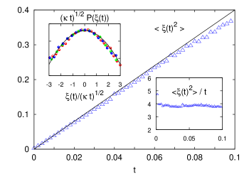
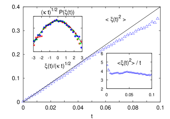
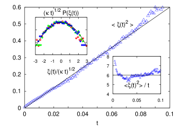
Following the procedure described in BBCF07 from the zero-field lines we obtain an ensemble of curves in the the half plane which are expected to converge in the scaling limit to chordal SLE. Then we extract the driving of the corresponding Loewner equation. As shown in Figures 8 and 9 the driving has Gaussian statistics with variance . For all the cases considered with we found , which is in agreement with the fractal dimension observed.
As a further test we study the statistics of the winding angle of the zero-isolines. The winding angle is defined as the degree with which the curve wind in the complex plane about a point DB02 ; WW03 . The asymptotic distribution for the winding angle at long distance along the curve is Gaussian, with variance . As shown in Figures 10 and 11 we found that its variance grows like , thus supporting the conjecture , and is not compatible with the prediction .

This model provides an example of non-trivial relation between the scaling exponent of the field and the fractal dimension of its isolines. For the scaling exponent varies in the range , but the fractal dimension remains constant , at variance with what one would expect from the relation which holds for Gaussian random field. The crucial difference is that the scalar field is not random, but is the result of turbulent dynamics.
Our findings can be understood in Lagrangian terms. The scaling exponent of the velocity field is . For the scaling exponent is positive, and therefore velocity difference scales as . Two Lagrangian trajectories moving in such velocity field separate according to the Richardson law . Conversely for , the exponent is negative (that is the velocity is a small-scale field like vorticity in Navier-Stokes), and velocity differences are independent of the separation . Lagrangian trajectories will separate as . Perimeter and gyration radius of clusters can be related by assuming that their ratio , which is proportional to the number of folds, grows as a random walk, i.e. as . Gyration radius grows as two-point distance , which gives for and for .
The property of conformal invariance of the isolines is therefore determined by the underlying dynamics of the field. As a test we took the field and randomize its phases in Fourier space. This procedure does not change the scaling exponent of the field, but destroys all the correlations generated by the turbulent dynamics. The isolines of this randomized field are no more conformal invariant, but their fractal dimension recover the prediction for Gaussian random field (see inset of Figure 6).
Under the hypothesis that the isoline of the scalar field are SLE curves one can obtain a conjecture for their universality class from the formula for the fractal dimension of the outer perimeter , which holds for D00 . One obtains for and for , which are in agreement with our findings ( and ) and with previous results ().
Approach based on Schramm-Loewner Evolution provides a refreshingly novel geometric insight into the statistics of turbulence and hints at deep symmetry aspects of 2d flows which we are yet far from understanding.
References
- (1) O. Schramm, Israel J. Math. 118, 221–288 (2000).
- (2) J. Cardy, Ann. Physics 318, 81 (2005).
- (3) M. Bauer and D. Bernard, Phys. Rep., submitted (2006); math-ph/0602049
- (4) D. Bernard et al, Nature Physics, 2, 124 (2006)
- (5) D. Bernard et al, Phys. Rev. Lett. 98, 024501 (2007).
- (6) G. Falkovich, Rus. Math Surv 62 497 (2007); J Phys A: Math Theor 42 123001 (2009).
- (7) P. Constantin, ”Geometric Statistics in Turbulence” SIAM review 36, 1 (1994).
- (8) R. T. Pierrehumbert, I. M. Held, and K. L. Swanson, Chaos, solitons and fractals 4, 1111 (1994)
- (9) K. Gawȩdzki, private communication.
- (10) J. Kondev and C. L. Henley, Phys. Rev. Lett. 74, 4580 (1995)
- (11) B. Duplantier and I.A. Binder, Phys. Rev. Lett. 89, 264101 (2002)
- (12) B. Wieland, D.B. Wilson Phys. Rev. E 68, 2003 (2003)
- (13) B. Duplantier, Phys. Rev. Lett. 84, 1363 (2000)