Stable Hamiltonian structures in dimension three are supported by open books

1 Introduction

In dimension three, (cooriented) contact structures are closely related to open books via the following results, the first due to Thurston-Winkelnkemper [8] and the other ones due to Giroux [6]:

(1) Every open book supports a contact structure.

(2) Any two contact structures supported by the same open book are connected by a contact isotopy supported by the open book.

(3) Every contact structure is supported by an open book.

(4) Two open books supporting the same contact structure are isotopic after finitely many stabilizations.

In [3] we proved analogues of the first two results for stable Hamiltonian structures in dimension three:

(1’) Every open book supports a stable Hamiltonian structure realizing a given cohomology class and given signs at the binding components.

(2’) Any two stable Hamiltonian structures supported by the same open book in the same cohomology class and with the same signs at the binding components are connected by a stable homotopy supported by the open book.

In this paper we prove the analogue of the third result.

Theorem 1.1.

Every stable Hamiltonian structure on a closed oriented $3$-manifold is stably homotopic to one which is supported by an open book.

Definitions. Let us first explain the notions appearing in the statement; see [3] for more details and background.

Let $M$ denote a closed oriented $3$-manifold. A stable Hamiltonian structure (SHS) on $M$ is a pair $(\omega,\lambda)$ consisting of a closed 2-form $\omega$ and a 1-form $\lambda$ such that

$$\lambda\wedge\omega>0\qquad\text{and}\qquad\ker(\omega)\subset\ker(d\lambda).$$ (1)

It induces a canonical Reeb vector field $R$ generating $\ker(\omega)$ and normalized by $\lambda(R)=1$. Note that in dimension 3 the second condition in (1) is equivalent to

$$d\lambda=f\omega$$

for some $f\in C^{\infty}(M)$ which we write as $f=d\lambda/\omega$. A stable homotopy is a smooth family of SHS $(\omega_{t},\lambda_{t})$ such that the cohomology class of $\omega_{t}$ remains constant. (The condition on the cohomology class is natural for many reasons, e.g. to get invariance of symplectic field theory under stable homotopies). A SHS $(\omega,\lambda)$ with $0=[\omega]\in H^{2}(M;{\mathbb{R}})$ is called exact. Note that each contact form $\lambda$ (i.e. satisfying $\lambda\wedge d\lambda>0$) induces an exact stable Hamiltonian structure $(d\lambda,\lambda)$.

An open book decomposition of $M$ is a pair $(B,\pi)$, where $B\subset M$ is an oriented link (called the binding) and $\pi:M\setminus B\rightarrow S^{1}$ is a fibration satisfying the following condition near $B$: Each connected component $B_{l}$ of $B$ has a tubular neighbourhood $S^{1}\times D^{2}\hookrightarrow M$ with orienting coordinates $(\phi,r,\theta)$, where $\phi$ is an orienting coordinate along $S^{1}\cong B_{l}$ and $(r,\theta)$ are polar coordinates on $D^{2}$, such that on $(S^{1}\times D^{2})\setminus B_{l}$ we have $\pi(\phi,r,\theta)=\theta$. It follows that the closure of each fibre $\pi^{-1}(\theta)$ is an embedded compact oriented surface $\Sigma_{\theta}$ (called a page) with boundary $B$.

We call a SHS $(\omega,\lambda)$ supported by the open book $(B,\pi)$ if $\omega$ is positive on each fibre $\pi^{-1}(\theta)$. It follows that $\lambda$ is nowhere vanishing on the binding. Thus for every binding component $B_{l}$ we have a sign $s(B_{l})$ which is $+1$ iff $\lambda$ induces the orientation of $B_{l}$ as boundary of a page. We emphasize that this differs from the common notion in contact topology where one requires that all signs are $+1$. The results (i-iv) above in the contact case have to be understood for this more restrictive notion to which we will refer as positively supported. It is shown in [3] that in Theorem 1.1 we cannot achieve “positively supported”: There exists a stable Hamiltonian structure on $S^{3}$ which is not stably homotopic to one that is positively supported by an open book.

On the other hand, if an exact SHS is positively supported by an open book, then by results (1) and (2’) above it is stably homotopic to a positive contact structure (i.e. to a SHS of the form $(d\lambda,\lambda)$ for a positive contact form $\lambda$).

Example 1.2.

Consider an exact SHS $(\omega,\lambda)$ for which $\lambda$ defines a confoliation, i.e. $\lambda\wedge d\lambda\geq 0$ (see [4]). Then $(\omega,\lambda)$ is stably homotopic to a positive contact structure. To see this, note that the confoliation condition is equivalent to $f=d\lambda/\omega\geq 0$. This allows us to achieve positive signs at all binding components of the open book in Theorem 1.1 (see Remark 5.4), so the resulting SHS is positively supported by the open book and hence stably homotopic to a positive contact structure. The stable homotopy can also be constructed explicitly as follows: Write $\omega=d\alpha$. Then $\lambda_{t}:=\lambda+t\alpha$, $t\in[0,\varepsilon]$, defines for small $\varepsilon>0$ a homotopy of stabilizing forms from $\lambda$ to the positive contact form $\lambda_{\varepsilon}$, and $\bigl{(}(1-t)\omega+t\,d\lambda_{\varepsilon},\lambda_{\varepsilon}\bigr{)}$ yields a stable homotopy from $(\omega,\lambda_{\varepsilon})$ to $(d\lambda_{\varepsilon},\lambda_{\varepsilon})$.

Sketch of proof. The proof of Theorem 1.1 departs from a structure theorem proved in [3] (see Section 5): For each SHS $(\omega,\lambda)$ on a closed oriented 3-manifold $M$ we can change the 1-form $\lambda$ such that $M=\bigcup_{i}N_{i}\cup\bigcup_{j}U_{j}$ is a union of compact regions such that $(\omega,\lambda)$ is $T^{2}$-invariant on $U_{j}\cong[0,1]\times T^{2}$, and $d\lambda=c_{i}\omega$ on $N_{i}$ with constants $c_{i}\in{\mathbb{R}}$. We refer to the regions $U_{j}$ as integrable regions, and to the regions $N_{i}$ with $c_{i}=0$ (resp. $>0$, $<0$) as flat (resp. positive / negative contact) regions.

On a flat region we perturb and rescale $\lambda$ to make it integral and obtain a fibration over $S^{1}$. On a (positive or negative) contact region we use a relative version of Giroux’s existence theorem (3) above to produce an open book supporting the contact form $\lambda$ (and hence the SHS $(\omega,\lambda)$) which induces a fibration $T^{2}\to S^{1}$ on each boundary torus. Finally, we use techniques from [3] to extend the SHS and open books over the integrable regions $U_{j}$ to a SHS and supporting open book on $M$ (Section 6).

To prove the relative version of (3) we collapse a circle direction transverse to the Reeb direction $\partial N_{i}$ to obtain a closed contact manifold $(\bar{N}_{i},\bar{\lambda})$ (Section 4). Each boundary torus $T_{j}$ gives rise to a transverse knot $L_{j}$. We use Giroux’s existence theorem (3) to find a supporting open book for $(\bar{N}_{i},\bar{\lambda})$ and apply a result of Pavelescu [7] to braid the link $L=\cup L_{j}$ around its binding (Section 2). After standardizing $\bar{\lambda}$ near the resulting link (Section 3) we replace its components back by 2-tori to obtain the desired open book on $N_{i}$.

Acknowledgements. We thank Y. Eliashberg and J. Etnyre for fruitful discussions.

2 Braiding transverse knots around the binding of a contact open book

We will use the following terminology. A contact form $\alpha$ is supported by an open book $(B,\pi)$ if $\alpha$ restricts positively to the binding and $d\alpha$ restricts positively to the pages. A contact structure $\xi$ is supported by an open book if there exists a contact form defining $\xi$ which is supported by the open book. An oriented link $L$ is (positively) transverse to the contact structure $\xi$ if a defining contact form $\alpha$ restricts positively to $L$. An oriented link $L$ is braided around an open book $(B,\pi)$ if $L$ is disjoint from the binding and positively transverse to the pages, i.e. $d\pi$ restricts positively to $L$.

The goal of this section is to explain the following result from E. Pavelescu’s thesis [7].

Theorem 2.1.

Let $M$ be a closed oriented $3$-manifold and $\xi$ be a cooriented contact structure on $M$ supported by an open book $(B,\pi)$, and $L\subset M$ be a link positively transverse to $\xi$. Then there exist isotopies $(B_{t},\pi_{t},L_{t})_{t\in[0,1]}$ of open books $(B_{t},\pi_{t})$ supporting $\xi$ and links $L_{t}$ transverse to $\xi$ such that $(B_{0},\pi_{0},L_{0})=(B,\pi,L)$ and $L_{1}$ is braided around $(B,\pi)$.

Moreover, for every collection of suficiently large natural numbers $k_{1},\dots,k_{\ell}\geq K$, where $\ell$ is the number of components of $L$ and $K$ a constant depending on $(B,\pi,\xi,L)$, we can arrange that the intersection number of the $i$-th component of $L_{1}$ with a page of $(B_{1},\pi_{1})$ equals $k_{i}$.

Remark 2.2.

Pavelescu claims the stronger result that the open book $(B_{t},\pi_{t})=(B,\pi)$ can be fixed. As the proof in [7] contains some gaps, we repeat it below with some more details. The deformation of the open book is needed for technical reasons; it can be made $C^{1}$-small, and presumably be avoided with more work.

The proof in [7] is based on the following construction. Consider a contact form $\alpha$ supported by an open book $(B,\pi)$. Suppose that

$$\alpha=T(1-r^{2})(d\phi+r^{2}d\theta)$$

in a tubular neighbourhood $W=\{r\leq r_{0}\}$ of $B$, where $T>0$ is some constant and $(\phi,r,\theta)$ are (polar) coordinates near the respective binding components in which $\pi=\theta$. We define another neighbourhood

$$V:=\{r\leq r_{0}/2\}\subset\{r\leq r_{0}\}=W$$

of $B$. Let $f:[0,r_{0}]\to[0,1]$ be a nondecreasing function which equals $T(1-r^{2})r^{2}$ for $r\leq r_{0}/2$ and $1$ near $r=r_{0}$. It extends by $1$ over $M\setminus W$ to a function on $M$ that we also denote by $f$. Consider the family of contact structures

$$\xi_{t}:=\ker\alpha_{t},\qquad\alpha_{t}:=\alpha+tf\,d\theta,\qquad t\in[0,\infty).$$ (2)

By Gray’s stability theorem we know that there is a family of diffeomorphisms $\{\Psi_{t}\}_{t\in[0,\infty)}$ such that $\Psi_{t}$ pulls back $\alpha_{t}$ to a multiple of $\alpha_{0}=\alpha$. We need to analyse $\{\Psi_{t}\}$ more closely. Recall that $\Psi_{t}$ is given as the flow of the time-dependent vector field $X_{t}\in\xi_{t}$ defined by

$$i_{X_{t}}d\alpha_{t}=h_{t}\alpha_{t}-\dot{\alpha}_{t},\qquad h_{t}:=\dot{\alpha}_{t}(R_{t}),$$ (3)

where $R_{t}$ denotes the Reeb vector field of $\alpha_{t}$ and $\dot{\alpha}_{t}$ denotes the time derivative of $\alpha_{t}$.

Consider a page $\Sigma$ and note that $\alpha_{t}|_{\Sigma}=\alpha_{\Sigma}$, so all the $\alpha_{t}$ define the same characteristic foliation $\mathcal{F}=\xi\cap T\Sigma=\xi_{t}\cap\Sigma$ on $\Sigma$. Since $d\alpha_{t}|_{\Sigma}=d\alpha_{\Sigma}$ is positive, $R_{t}$ is positively transverse to $\Sigma$ and $\dot{\alpha}_{t}=f\,d\theta$ yields $h_{t}=f\,d\theta(R_{t})>0$. Contracting equation (3) with any vector $v\in\xi\cap T\Sigma$ we obtatain $d\alpha(X_{t},v)=0$, and since $v,X_{t}\in\xi$ and $d\alpha|_{\xi}$ is nondegenerate this implies that $v$ and $X_{t}$ are collinear. This shows that $X_{t}$ is tangent to the pages and spans the charateristic foliation. Moreover, the restriction of equation (3) to $\Sigma$ gives

$$i_{X_{t}}d\alpha|_{\Sigma}=h_{t}\alpha|_{\Sigma}.$$ (4)

Thus $X_{t}$ is determined by equation (4). In particular, each $X_{t}=h_{t}X$ is a positive multiple of the Liouville field $X$ tangent to the pages defined by

$$i_{X}d\alpha|_{\Sigma}=\alpha|_{\Sigma}.$$

A short computation shows $X=-\frac{1-r^{2}}{2r}\partial_{r}$ on $W$, so $X$ points into $V$ along $\partial V$. The key property of $X$ is that $L_{X}d\alpha|_{\Sigma}=d(i_{X}d\alpha|_{\Sigma})=d\alpha|_{\Sigma}$, i.e. $X$ expands the positive area form $d\alpha|_{\Sigma}$ on the page. This has the following dynamical consequences:

1. Each closed orbit of $X$ is repelling.

2. At each zero $p\in\Sigma$ of $X$ the linearization $d_{p}X|_{T\Sigma}$ has an eigenvalue with positive real part. If the eigenvalues are non-real, or both real and positive, this implies that $p$ is nondegenerate and $X$ flows out of $p$; we call such $p$ elliptic. If the eigenvalues are real with one positive and one non-positive we call $p$ hyperbolic; in this case there may be one or two flow lines converging to $p$ in forward time.

3. As a consequence of (i-ii) and the Poincaré-Bendixson Theorem, every flow line of $X$ which is not a zero or a closed orbit either enters $V$ in finite time or converges to a hyperbolic zero in forward time.

Now consider the $S^{1}$-family of pages $\Sigma_{\theta}:=\pi^{-1}(\theta)$, $\theta\in S^{1}$. For any $\theta\in S^{1}$ let $S_{\theta}$ denote the subset of $\Sigma_{\theta}$ consisting of zeroes, closed orbits, and flow lines converging to hyperbolic zeros in forward time. We set

$$S:=\cup_{\theta\in S^{1}}S_{\theta}$$ (5)

The following statement is crucial for the proof.

Lemma 2.3.

Let $U_{S}$ be an open neighbourhood of $S$ in $M\setminus B$. Then there exists $\tau\in[0,+\infty)$ such that $\Psi_{\tau}(M\setminus U_{S})\subset V$.

Proof.

By property (iii) above and compactness, there exists a constant $\tau_{0}>0$ such that each point in $M\setminus U_{S}$ reaches $V$ in time $\tau_{0}$ under the flow of $X$. To get the corresponding statement with the time-dependent vector field $X_{t}$ in place of $X$ we need to look at the behaviour of the length of $X_{t}$ as $t\to+\infty$. Since the $d\theta$ component of $\alpha_{t}$ goes to $\infty$ as $t\to 0$, we get that $R_{t}\to 0$ as $t\to\infty$. ¿From

$$1=\alpha_{t}(R_{t})=\alpha(R_{t})+tf\,d\theta(R_{t})$$

and $\alpha(R_{t})\to 0$ as $t\to\infty$ we see that $h_{t}=f\,d\theta(R_{t})=O(t^{-1})$ as $t\to\infty$ on $M\setminus B$. Since $\int_{1}^{\infty}\frac{1}{t}dt=\infty$, there exists a constant $\tau>0$ such that each point in $M\setminus U_{S}$ reaches $V$ in time $\tau$ under the flow $\Psi_{t}$ generated by $X_{t}$. ∎

Besides the preceding discussion, we will also use in the proof the following 3 lemmas which correspond to Lemmas 4.9, 4.10 and 4.12 in [3], respectively.

Lemma 2.4.

For all $\delta,\varepsilon>0$ there exists a smooth function $\rho:[0,\delta]\rightarrow[0,1]$ with the following properties: $\rho$ is nonincreasing, constant $1$ in a neighbourhood of $0$, constant $0$ in a neighbourhood of $\delta$, and

$$|x\rho^{\prime}(x)|<\varepsilon$$

for all $x\in[0,\delta]$.

Lemma 2.5.

Let $\alpha$ be a positive contact form on $U=S^{1}\times D^{2}$ satisfying $d\theta\wedge d\alpha>0$ and $T:=\int_{S^{1}\times\{0\}}\alpha>0$. Then there exists a homotopy rel $\partial U$ of contact forms $\alpha_{t}$ satisfying $d\theta\wedge d\alpha_{t}>0$ such that $\alpha_{0}=\alpha$ and

$$\alpha_{1}=T(r^{2}d\theta+(1-r^{2})d\phi)$$

near $S^{1}\times\{0\}$.

Lemma 2.6.

Let $\phi$ be the angular coordinate on $S^{1}$ and $(r,\theta)$ be polar coordinates on $D^{2}$. Let $\sigma:[0,1]\to{\mathbb{R}}$ be a function, constant near $r=0$ and supported in $[0,\delta]$, with $|r\sigma^{\prime}(r)|\leq\varepsilon$. Let $\alpha_{0},\alpha_{1}$ be two contact forms on $S^{1}\times D^{2}$ satisfying $d\theta\wedge d\alpha_{i}\geq\beta>0$, $i=0,1$ and $\alpha_{1}-\alpha_{0}=O(r^{2})$ near $\{r=0\}$. Then for $\delta,\varepsilon$ sufficiently small the 1-form $\alpha:=(1-\sigma(r))\alpha_{0}+\sigma(r)\alpha_{1}$ is contact and satisfies $d\theta\wedge d\alpha>0$.

After these preparations, we now turn to the

Proof of Theorem 2.1.

Step 0. We first put the open book $(B,\pi)$ into nice position with respect to $\xi$. After a small transverse isotopy (fixing $(B,\pi,\xi)$) we may assume that the link $L$ does not intersect the binding $B$. Let $\alpha$ be a contact form defining $\xi$ and supported by $(B,\pi)$. By Lemma 2.5 we find a homotopy of contact forms $\{\alpha_{t}\}_{t\in[0,1]}$ supported by $(B,\pi)$, fixed outside a neighbourhood of $B$, with $\alpha_{0}=\alpha$ and

$$\alpha_{1}|_{W}=T(r^{2}d\theta+(1-r^{2})d\phi)$$

for some neighbourhood $W=\{r\leq r_{0}\}$ of $B$ and some locally constant function $T>0$ on $W$, where $(\phi,r,\theta)$ are the standard open book coordinates near $B$. Using Lemma 2.6, we can further deform the contact form $\alpha_{1}$, through contact forms supported by $(B,\pi)$ and fixed outside a neighbourhood of $B$, to a contact form $\alpha_{2}$ satisfying

$$\alpha_{2}|_{W}=T(1-r^{2})(r^{2}d\theta+d\phi)$$

(after shrinking $W$). Finally, we perturb $\alpha_{2}$, keeping it fixed near $B$, to a contact form $\alpha_{3}$ for which the charactistic foliations on the pages are sufficiently generic (in a sense that is made precise below).

After applying Gray’s theorem, we may assume that $\xi$ and $L$ are fixed and the open book is moving by an isotopy. We rename the new open book back to $(B,\pi)$ and the new contact form $\alpha_{3}$ back to $\alpha$.

After this preparatory step, we will keep $(B,\pi,\xi)$ fixed and only deform the transverse link $L$. More precisely, we will construct a family $(\xi_{t},L_{t})_{t\in[0,A]}$ of contact structures $\xi_{t}$ and links $L_{t}$ in $M$ with the following properties:

(a)

there exists a family of diffeomorphisms $(\psi_{t})_{t\in[0,A]}$ with

$$\psi_{0}={{\mathchoice{\rm 1\mskip-4.0mul}{\rm 1\mskip-4.0mul}{\rm 1\mskip-4.5mul}{\rm 1\mskip-5.0mul}}},\quad\psi_{t}^{*}\xi_{t}=\xi,\quad\psi_{t}(B)=B,\quad\pi\circ\psi_{t}=\pi;$$

(b)

$L_{0}=L$ and $L_{t}$ is transverse to $\xi_{t}$ for all $t\in[0,A]$;

(c)

$L_{A}$ is braided around $(B,\pi)$ and the intersection number the $i$-th component of $L_{A}$ with a page is $k_{i}$.

Then the links $L_{t}^{\prime}:=\psi_{t}^{-1}(L_{t})$ satisfy $L_{0}^{\prime}=L$, $L_{t}^{\prime}$ is transverse to $\psi_{t}^{*}\xi_{t}=\xi$ for all $t\in[0,A]$, and $L_{A}^{\prime}$ is braided around $\bigl{(}\psi_{A}^{-1}(B),\pi\circ\psi_{A}\bigr{)}=(B,\pi)$ with intersection numbers $k_{i}$. Thus $L_{t}^{\prime}$ is the desired isotopy.

We construct the family $(\xi_{t},L_{t})_{t\in[0,A]}$ in 6 steps.

Step 1. Recall that from Step 0 we have a contact form $\alpha$ defining $\xi$ supported by $(B,\pi)$ which is given by

$$\alpha=T(1-r^{2})(d\phi+r^{2}d\theta)$$

in a tubular neighbourhood $W=\{r\leq r_{0}\}$ of $B$ not meeting $L$. Let us call an arc $\gamma$ of $L$ good if $\gamma$ is positively transverse to the pages, and bad otherwise. Let $L_{g}$ denote the union of all good arcs and set $L_{b}:=L\setminus L_{g}$. Since transversality is an open condition, we know that $L_{g}$ is a union of open arcs and (after a small isotopy of $L$) we may assume that $L_{b}$ is a union of closed arcs. Our objective is to achieve $L_{b}\cap S=\emptyset$, so that we can use Lemma 2.3 to push $L_{b}$ into a smaller neighbourhood

$$V:=\{r\leq r_{0}/2\}$$

of $B$.

By the last generic perturbation in Step 0 we can achieve that the set $S$ is a union of submanifolds of dimensions $0,1,2$ of the following types:

S(1)

finitely many zeroes of birth-death type;

S(2)

nondegenerate (elliptic or hyperbolic) zeroes varying in 1-dimensional families with $\theta$;

S(3)

isolated flow lines converging in forward time to birth-death type zeroes;

S(4)

isolated flow lines converging in forward and backward time to nondegenerate hyperbolic zeroes;

S(5)

nondegenerate closed orbits varying in 1-dimensional families with $\theta$;

S(6)

flow lines converging in forward time to nondegenerate hyperbolic zeroes (and in backward time to elliptic zeroes or closed orbits) varying in 1-dimensional families with $\theta$.

Note that, for each stratum $S(n)$, $\overline{S(n)}\setminus S(n)$ is contained in the union of strata $S(m)$ with $m<n$. We will successively make $L_{b}$ disjoint from $S(1),\dots,S(6)$. To begin, we make $L_{b}$ disjoint from the $0$- and $1$-dimensional strata $S(1),\dots,S(4)$ simply by a small perturbation of $L$.

Step 2. Let $\mathcal{P}=S(5)$ be the union of closed orbits of $X$. Each connected component of $\mathcal{P}$ is an embedded $2$-torus in $M$ fibered over $S^{1}$ by $\pi$. Consider a point $p\in\mathcal{P}$ belonging to a page $\Sigma$. Note that the three planes $T_{p}\Sigma$, $\xi_{p}$ and $T_{p}\mathcal{P}$ all contain the line ${\mathbb{R}}X(p)$, so their intersection with a plane $E\subset T_{p}M$ transverse to $X(p)$ gives three lines in $E$.

Recall that the contact structures $\xi_{t}=(\Psi_{t})_{*}\xi$ defined above (see equation (2)) converge at $p$ to $T_{p}\Sigma$ as $t\to\infty$. After applying the homotopy $\bigl{(}\xi_{t},L_{t}=\Psi_{t}(L)\bigr{)}$, $t\in[0,\tau]$, for sufficiently large $\tau$ and renaming $(\xi_{\tau},L_{\tau})$ back to $(\xi,L)$, we may hence assume that at all points $p\in\mathcal{P}$ the three lines corresponding to $\Sigma,\xi,\mathcal{P}$ (and their coorientations) are ordered as in Figure 1).

Figure 1: Wrinkling

Step 3. After a perturbation of $L$ we may assume that the intersection $L_{b}\cap\mathcal{P}$ is transverse. Consider a point $p\in L_{b}\cap\mathcal{P}$. Pick local coordinates $(x,y,z)\in{\mathbb{R}}^{3}$ near $p=(0,0,0)$ in which $\pi(x,y,z)=z$ and $\mathcal{P}=\{y=0\}$, so $X(p)$ points in the $x$-direction. By Step 2, the intersections of $T_{p}\Sigma$, $\xi_{p}$ and $T_{p}\mathcal{P}$ with the plane $\{x=0\}$ are ordered as in Figure 1. After a further coordinate change near $p$ we may assume that near $p$ the curve $L_{b}$ is a straight line segment contained in the plane $\{x=0\}$. After zooming in near $0$ and rescaling, we may assume that the contact planes in the neighbourhood are $C^{0}$-close to $\xi_{p}$. Now we modify $L_{b}$ near $p$ within the plane $\{x=0\}$ as shown in Figure 1. The new arc $L_{b}^{\prime}$ is transversely isotopic to $L_{b}$, by an isotopy fixed outside the neighbourhood of $p$ and always intersecting $\mathcal{P}$ transversely at the only point $p$, and $L_{b}^{\prime}$ is good near the intersection point $p$.

After applying this wrinkling operation to all intersections with $\mathcal{P}$, we may hence assume that $L$ avoids a closed neighbourhood $U_{\mathcal{P}}$ of $S(1)\cup\dots\cup S(5)$.

Step 4. After Step 3 and a perturbation of $L$, the curve $L_{b}$ intersects the 2-dimensional submanifold $S(6)$ transversely in finitely many points in $M\setminus U_{\mathcal{P}}$. Thus we can repeat steps 2 and 3 with $S(5)$ replaced by $S(6)$ to make $L$ disjoint from an open neighbourhood $U_{S}$ of $S$.

Step 5. Now we are in the position to use the flow $\Psi_{t}$ of $X_{t}$ to push $L_{b}$ into $V$. According to Lemma 2.3 there exists $\tau>0$ such that $\Psi_{\tau}(M\setminus U_{S})\subset V$ and thus $\Psi_{\tau}(L_{b})\subset V$. Since $\Psi_{t}$ preserves the binding and pages of the open book $(B,\pi)$, the homotopy $(\xi_{t},L_{t})_{t\in[0,\tau]}$ defined by

$$\xi_{t}:=(\Psi_{t})_{*}\xi,\qquad L_{t}:=\Psi_{t}(L)$$

satisfies properties (a) and (b) above. Moreover, the bad (unbraided) part of $\mathcal{L}_{\tau}$ is given by $\Psi_{\tau}(L_{b})$ and hence contained in $V$. Note that the new contact form $\alpha_{\tau}$ is given on $V$ by

$$\alpha_{\tau}=T(1-r^{2})\Bigl{(}d\phi+(1+\tau)r^{2}d\theta\Bigr{)}.$$

Step 6. Consider the contact structure $\xi_{\tau}=\ker\alpha_{\tau}$ from Step 5 on $V=S^{1}\times D^{2}$. After rescaling in $r$ we may assume that $\xi_{\tau}=\xi_{st}=\ker(d\phi+r^{2}d\theta)$. By a result of Bennequin ([2], see also [7] for a short exposition) we can transversely isotope $L_{\tau}$ relative to $\partial V$ (fixing $\xi_{\tau}$) to a link which is disjoint from the binding $\{r=0\}$ and positively transverse to the pages $\{\theta=const\}$ in $V$. Since $L_{\tau}$ was already braided outside $V$, the resulting link $L_{A}\subset M$ is braided around $(B,\pi)$.

Finally, let $K$ be the maximum of the intersection numbers of the components of $L_{A}$ with a page of $(B,\pi)$. Then for any integer $k_{i}\geq K$ we can further transversely isotope the $i$-th component (pulling it through $B$) in such a way that at the end it is again braided and its intersection number with a page equals $k_{i}$. This concludes the proof of Theorem 2.1. ∎

3 Standardization of a contact open book near a transverse knot

In this section we prove the following improvement of Theorem 2.1.

Corollary 3.1.

Let $(M,\alpha)$ be a closed oriented contact $3$-manifold. Let $L=\cup_{i=1,\dots,\ell}L_{i}\subset M$ be a link (with components $L_{i}$) positively transverse to the contact structure $\ker\alpha$. Then there exists a natural number $K$ with the following property. For every collection of numbers $k_{i}\geq K$, $i=1,\dots,\ell$, there exists a contact form $\beta$ with $\ker\beta=\ker\alpha$ and an open book $(B,\pi)$ supporting $\beta$ such that $L$ is disjoint from $B$ and positively transverse to the pages, and the intersection number of $L_{i}$ with a page is $k_{i}$. Moreover, in coordinates $(\theta,r,\phi)\in S^{1}\times D^{2}$ near $L_{i}=S^{1}\times\{0\}$ we have

$$\beta=\alpha=f(d\theta+r^{2}d\phi)\quad\text{and}\quad\pi(\theta,r,\phi)=k_{i}\theta.$$

Proof.

By Theorem 2.1 we find a contact form $\beta$ and an open book $(B,\pi)$ having all the properties in the corollary except the last one, i.e. $\beta$ need not agree with $\alpha$ near $L$ and $\pi$ need not be standard as above. Consider a component $L_{i}$ of $L$. It has a tubular neighbourhood $V\cong S^{1}\times D^{2}_{\delta}$ with coordinates $\theta\in S^{1}$ and polar coordinates $(r,\phi)$ on the disk $D^{2}_{\delta}$ in which the contact structure $\xi=\ker\beta$ is given by

$$\xi_{\rm st}=\ker\alpha_{\rm st},\qquad\alpha_{\rm st}=d\theta+r^{2}d\phi.$$

By Lemma 3.2 below there exist

• an open book $(B,\pi^{\prime})$ on $M$ which agrees with $(B,\pi)$ outside $V$ such that $\pi^{\prime}(\theta,r,\phi)=k_{i}\theta$ near $L_{i}$, and

• a contact form $\beta^{\prime}$, supported by $(B,\pi^{\prime})$ and defining $\xi$, which coincides with $\beta$ outside $V$ and with $\alpha_{\rm st}$ near $L_{i}$.

By Lemma 3.3 below, $\beta^{\prime}$ can be modified near $L_{i}$ to a contact form $\beta^{\prime\prime}$, still supported by $(B,\pi^{\prime})$ and defining $\xi$, such that $\beta^{\prime\prime}=\alpha$ near $L_{i}$. Then $\beta^{\prime\prime}$ and $(B,\pi^{\prime})$ have the desired properties. ∎

It remains to prove the two lemmas used in the proof of Corollary 3.1. We consider a tubular neighbourhood $V=S^{1}\times D^{2}_{\delta}$ of the knot $K=\{r=0\}$ with coordinates $(\theta,r,\phi)$ and the contact structure $\xi_{\rm st}=\ker\alpha_{\rm st}$ as above. Note that an open book without binding on $V$ is simply a submersion $\pi:V\to S^{1}$, and it supports a contact form $\alpha$ iff $d\pi\wedge d\alpha>0$.

Lemma 3.2.

Let $\alpha$ be a contact form on $V$ defining $\xi_{\rm st}$ and $\pi:V\to S^{1}$ be a submersion such that $d\pi\wedge d\alpha>0$ and $\pi|_{K}:K\to S^{1}$ is a covering of degree $n\in{\mathbb{N}}$. Then there exist

• a submersion $\pi^{\prime}:V\to S^{1}$ which agrees with $\pi$ near $\partial V$ such that $\pi^{\prime}(\theta,r,\phi)=n\theta$ near $K$, and

• a contact form $\alpha^{\prime}$ on $V$, defining $\xi_{\rm st}$ and satisfying $d\pi^{\prime}\wedge d\alpha^{\prime}>0$, which coincides with $\alpha$ near $\partial V$ and with $\alpha_{\rm st}$ near $K$.

Note that for the submersion $\pi^{\prime}(\theta,r,\phi)=n\theta$ the condition $d\pi^{\prime}\wedge d\alpha^{\prime}>0$ is just $d\theta\wedge d\alpha^{\prime}>0$.

Lemma 3.3.

Let $\alpha_{0},\alpha_{1}$ be two contact forms on $V$ defining $\xi_{\rm st}$ such that $d\theta\wedge d\alpha_{i}>0$ for $i=0,1$. Then there exists a contact form $\alpha$ on $V$, defining $\xi_{\rm st}$ and satisfying $d\theta\wedge d\alpha>0$, which coincides with $\alpha_{0}$ near $\partial V$ and with $\alpha_{1}$ near $K$.

Proof of Lemma 3.3.

We write $\alpha_{i}=f_{i}\alpha_{\rm st}$ for functions $f_{i}:V\to{\mathbb{R}}_{+}$ and $\alpha=f\alpha_{\rm st}$, where

$$f:=\bigl{(}1-\rho(r)\bigr{)}f_{0}+\rho(r)f_{1}.$$

Here $\rho:[0,\delta]\to[0,1]$ is a nonincreasing function as in Lemma 2.4 which equals $1$ near $0$ and $0$ near $\delta$ and satisfies $|r\rho^{\prime}(r)|\leq\varepsilon$, for arbitrarily small constants $\varepsilon,\delta>0$ that will be chosen below. Now

$$d\theta\wedge d\alpha=d\theta\wedge\frac{\partial f}{\partial r}dr\wedge r^{2}d\phi+f\,d\theta\wedge 2r\,dr\wedge d\phi=\left(2f+r\frac{\partial f}{\partial r}\right)d\theta\wedge r\,dr\wedge d\phi$$

is positive iff

$$2f+r\frac{\partial f}{\partial r}>0.$$ (6)

To show (6) we estimate with positive constants $c_{0},c_{1},c_{2}$ depending only on $f_{0},f_{1}$:

$$2f\geq 2{\rm min}\{{\rm min}_{V}f_{0},{\rm min}_{V}f_{1}\}\geq c_{0}>0,$$

$$\left|r\frac{\partial f}{\partial r}\right|\leq r\left|(1-\rho)\frac{\partial f_{0}}{\partial r}+\rho\frac{\partial f}{\partial r}\right|+|r\rho^{\prime}(r)|\,|f_{1}-f_{0}|\leq c_{1}\delta+c_{2}\varepsilon.$$

Thus for $\varepsilon,\delta$ sufficiently small (6) holds and Lemma 3.3 follows. ∎

Proof of Lemma 3.2.

Step 1. We make a coordinate change of $V$ of the form

$$(\theta,r,\phi)\mapsto\bigl{(}\Theta=\Theta(\theta),r,\phi\bigr{)},$$

where the diffeomorphism $\theta\mapsto\Theta(\theta)$ of $K\cong S^{1}$ is chosen in such a way that in the new coordinates the covering on $K$ is given by

$$\pi(\Theta,0,\phi)=n\Theta.$$ (7)

Note that $d\theta\wedge d\alpha$ is positive at $\{r=0\}$ by the contact condition, so after shrinking $V$ we may assume it is positive on the whole of $V$ and thus

$$d\Theta\wedge d\alpha=\Theta^{\prime}(\theta)d\theta\wedge d\alpha>0.$$

Step 2. Since the 1-forms $d\pi$ and $n\,d\Theta$ are cohomologous, we have

$$d\pi=n\,d\Theta+df$$

for some function $f:V\to{\mathbb{R}}$, hence (after adding a constant to $f$ if necessary) $\pi=n\Theta+f$. Equation (7) then implies that $f|_{K}=0$, i.e. we have $|f|\leq C_{f}r$ for some constant $C_{f}$ depending only on $f$. We take a nondecreasing function $\rho:[0,\delta]\to[0,1]$ as provided by Lemma 2.4 (replacing $\rho$ by $1-\rho$) which equals $0$ near $r=0$ and $1$ near $r=\delta$ and satisfies $r\rho^{\prime}(r)\leq\varepsilon$. Consider the map

$$\pi_{1}:=n\Theta+\rho(r)f:V\to S^{1}.$$

Claim: For $\varepsilon$ sufficiently small we have $d\pi_{1}\wedge d\alpha>0$.

To prove this, we use $\alpha=h(d\theta+r^{2}d\phi)$ to write out

$$d\theta_{1}\wedge d\alpha =d(n\Theta+\rho f)\wedge d\alpha$$ (8)

$$=(n\,d\Theta+\rho\,df)\wedge d\alpha+f\,d\rho\wedge d\Bigl{(}h(d\theta+r^{2}d\phi)\Bigr{)}$$ (9)

$$=(n\,d\Theta+\rho\,df)\wedge d\alpha+f\rho^{\prime}(r)[h_{\phi}-r^{2}h_{\theta}]dr\wedge d\phi\wedge d\theta.$$ (10)

Since both expressions

$$S_{1}:=n\,d\Theta\wedge d\alpha$$

and

$$S_{2}:=(nd\Theta+df)\wedge d\alpha=d\pi\wedge d\alpha$$

are positive, their convex combination

$$(1-\rho)S_{1}+\rho S_{2}=(n\,d\Theta+\rho\,df)\wedge d\alpha\geq min(S_{1},S_{2})$$

is bounded from below by a constant independent of $\rho$. So it remains to estimate the last summand in (8). Note that the $\phi$-derivative of any function vanishes at $\{r=0\}$ and thus we have an estimate $|h_{\phi}|\leq C_{h}r$ with a constant $C_{h}$ depending only on $h$. Using this as well as $|f|\leq C_{f}r$ and $r\rho^{\prime}(r)\leq\varepsilon$ we estimate

$$|f\rho^{\prime}(r)[h_{\phi}-r^{2}h_{\theta}]|\leq C_{f}r\rho^{\prime}(r)C_{h}r\leq C_{f}C_{h}\varepsilon r.$$

Since $r\,dr\wedge d\phi\wedge d\theta$ is a smooth volume form, this shows that the last summand in (8) becomes arbitrarily small for $\varepsilon$ small and thus proves the claim.

Thus $\pi_{1}:V\to S^{1}$ is a submersion, satisfying $d\pi_{1}\wedge d\alpha>0$, which agrees with $\pi$ near $\partial V$ and with $n\Theta$ near $K$. After shrinking $V$ and renaming $\pi_{1}$ back to $\pi$ we may hence assume that $\pi=n\Theta$ on $V$.

Step 3. Note that, after Step 2, $\alpha$ and $\alpha_{\rm st}$ are two contact forms defining $\xi_{\rm st}$ with $d\Theta\wedge\alpha>0$ and $d\Theta\wedge\alpha_{\rm st}>0$. So by Lemma 3.3 (in coordinates $(\Theta,r,\phi)$) we find a contact form $\beta$ on $V$, defining $\xi_{\rm st}$ and satisfying $d\theta\wedge d\beta>0$, which coincides with $\alpha$ near $\partial V$ and with $\alpha_{\rm st}$ near $K$. After shrinking $V$ and renaming $\beta$ back to $\alpha$, we may hence assume that $\alpha=\alpha_{\rm st}$ and $\pi=n\Theta$ on $V$.

Step 4. It remains to modify $\pi$ such that it equals $n\theta$ near $K$. The argument is similar to Step 2 but simpler: The forms $d\Theta$ and $d\theta$ are cohomologous, so we have $n\,d\Theta=n\,d\theta+df$ for some function $f$. In other words (after adding a constant to $f$ if necessary) $n\Theta=n\theta+f$. We define

$$\pi^{\prime}:=n\theta+\rho(r)f:V\to S^{1}$$

with a cutoff function $\rho$ as in Step 2. Since $d\alpha_{\rm st}=2r\,dr\wedge d\phi$ we have
$f\,d\rho\wedge d\alpha_{\rm st}=0$ and thus

$$d\pi^{\prime}\wedge d\alpha_{\rm st}=(n\,d\theta+\rho\,df)\wedge d\alpha_{\rm st},$$

which is a convex combination of the positive terms $n\,d\theta\wedge d\alpha_{\rm st}$ and $n\,d\Theta\wedge d\alpha_{\rm st}$ and hence positive. This concludes the proof of Lemma 3.2. ∎

4 Contact open books with boundary

Consider an oriented contact 3-manifold $(N,\alpha)$ whose boundary $\partial N=T_{1}\amalg\dots\amalg T_{\ell}$ is a union of 2-tori. We assume that $\alpha$ is $T^{2}$-invariant near each boundary component $T_{i}$, i.e. there exists a collar neighbourhood $K_{i}\cong[l_{i},R_{i}]\times T^{2}$ of $T_{i}=\{r=l_{i}\}\cong T^{2}$ with oriented coordinates $(r,\phi,\theta)$ in which $\alpha$ is given by

$$\alpha_{h}=h_{1}(r)d\phi+h_{2}(r)d\theta$$ (11)

for some immersion $h:[l_{i},R_{i}]\to{\mathbb{C}}$ satisfying

$$h_{1}^{\prime}h_{2}-h_{2}^{\prime}h_{1}>0.$$ (12)

(The immersion $h$ of course depends on $i$, but we suppress this dependence to keep the notation simple). We are interested in $\alpha$ that are supported by an open book decomposition $(B,\pi)$ in the usual sense (i.e. $\alpha>0$ on the binding $B$ and $d\alpha>0$ on the interior of the pages), where $B\subset{\rm int\,}N$ and the projection $\pi:N\setminus B\to S^{1}$ is in the above coordinates near each $T_{i}$ a linear projection $\pi(r,\phi,\theta)=a_{1}\phi+a_{2}\theta$. Here $a\in{\mathbb{Z}}^{2}$ is some integer vector (again depending on $i$) and positivity of $d\alpha$ on the pages, $d\pi\wedge d\alpha>0$, is equivalent to

$$h_{1}^{\prime}a_{2}-h_{2}^{\prime}a_{1}>0.$$

(Such “relative contact open books” were previously considered in [9, 1]). After a linear coordinate change on $T_{i}$ we may then assume that $a=(0,n_{i})$ for some $n_{i}\in{\mathbb{N}}$, so $\pi(r,\phi,\theta)=n_{i}\theta$ and the positivity condition $d\theta\wedge d\alpha>0$ becomes

$$h_{1}^{\prime}>0.$$ (13)

Note that the page $\Sigma$ of the open book has two kinds of boundary components: those that get collapsed to binding components, and others that give rise to the boundary tori $T_{i}$.

Recall Giroux’s result [6] that for any cooriented contact structure on a closed oriented 3-manifold (without boundary) there exists a defining contact form which is supported by an open book. The goal of this section is to prove the following relative version.

Proposition 4.1.

Let $(N,\alpha)$ be a compact oriented contact manifold with toric boundary $\partial N=T_{1}\amalg\dots\amalg T_{\ell}$ as above, i.e. there exist collar neighbourhood $K_{i}\cong[l_{i},R_{i}]\times T^{2}$ of $T_{i}=\{r=l_{i}\}\cong T^{2}$ on which $\alpha$ is given by (11). Assume that on each $K_{i}$ we have $d\theta\wedge d\alpha>0$ (i.e. $h_{1}^{\prime}>0$).

Then there exists a natural number $K$ such that for any collection $\{n_{i}\}_{i=1,\dots,\ell}$ of natural numbers with $n_{i}\geq K$ there exist a homotopy of contact form $\alpha_{t}$, $t\in[0,1]$, and an open book decomposition $(B,\pi)$ of $N$ with the following properties:

1. The contact form $\alpha_{1}$ is supported by the open book decomposition $(B,\pi)$. Moreover, $d\alpha_{1}=d\alpha$ near $\partial N$.

2. Near $T_{i}$ the fibration $\pi$ is given by $\pi(\theta,r,\phi)=n_{i}\theta$.

3. $\alpha_{0}=\alpha$, and $\alpha_{t}$ is $T^{2}$-invariant near $\partial N$ for all $t$.

4. Writing $\alpha=h_{1}(r)d\phi+h_{2}(r)d\theta$ and $\alpha^{t}=h_{1}^{t}(r)d\phi+h_{2}^{t}(r)d\theta$ near $T_{i}$, we have $h_{1}^{1}(l_{i})>0$, and if $h_{1}(l_{i})>0$ then $h_{1}^{1}(l_{i})<h_{1}(l_{i})$. Moreover, if $h_{1}(l_{i})\leq 0$, then $(h^{t})^{\prime}(l_{i})$ makes one full negative (i.e. clockwise) turn in the $(h_{2},h_{1})$ plane as $t$ runs from $0$ to $1$. If $h_{1}(l_{i})>0$, then we have a choice: we can choose $(h^{t})^{\prime}(l_{i})$ to have rotation number $-1$ or $0$.

5. If on some $T_{i}$ we have $h(r)=((r-l_{i}),1)$, then instead of (iv) the $T^{2}$-invariant homotopy $\alpha_{t}$ near $T_{i}$ can be chosen to be constant.

Proof.

Special case. First we treat the special case that $h(r)=((r-l_{i}),1)$ near each $T_{i}$. After a shift in the $r$ coordinate by $l_{i}$ we may assume that $\alpha=d\theta+rd\phi$ and $r\in[0,R_{i}]$. We remove the torus $\{0\}\times T^{2}$ and on the remaining $(0,R_{i}]\times T^{2}$ we do a coordinate change $r_{1}:=r^{1/2}$ and then rename $r_{1}$ back to $r$. Now the $1$-form $\alpha$ looks like $d\theta+r^{2}d\phi$. So it extends to the solid torus obtained by collapsing the $\phi$-direction in the removed torus $\{0\}\times T^{2}$. This gives rise to a closed contact manifold $(\bar{N},\bar{\alpha})$ with a transverse link $K_{1}\amalg\dots\amalg K_{\ell}$ obtained from the $T_{i}$. We apply Corollary 3.1 to obtain a contact form $\bar{\beta}$ on $\bar{N}$, defining the same contact structure as $\bar{\alpha}$ and supported by an open book $(\bar{B},\bar{\pi})$, such that $\bar{\beta}=\bar{\alpha}$ and $\bar{\pi}=n_{i}\theta$ near $K_{i}$. Replacing $K_{i}$ back by $T_{i}$ and changing coordinates back from $r^{1/2}$ to $r$ yields a contact homotopy $\alpha_{t}$ (by linear interpolation from $\bar{\alpha}$ to $\bar{\beta}$) and open book satisfying conditions (i-iii) and (v) in the proposition. This was “dream situation” in which we did not have to worry how to get back from $\bar{N}$ to $N$. Now we turn to the

General case. Consider one neighbourhood $K_{i}=[l_{i},R_{i}]\times T^{2}$. After a shift we may assume that $l_{i}>0$. We consider the solid torus $S^{1}\times D^{2}$ with coordinates $\theta\in S^{1}$ and polar coordinates $(r,\phi)$ on $D^{2}$, where $r\in[0,l_{i}]$, so that we can write $S^{1}\times D^{2}=\{r\in[0,l_{i}]\}$. We identify the boundary of this solid torus with $T_{i}$ via the identity map. Gluing in these solid tori for all $i$ gives us a closed manifold $\bar{N}$. Let $L_{i}$ denote the core circle $\{r=0\}$ of the solid torus $\{r\in[0,l_{i}]\}$. We consider the union of this solid torus with the collar neighbourhood of the respective boundary component

$$V_{i}:=K_{i}\cup\{r\in[0,l_{i}]\}=\{r\in[0,R_{i}]\}.$$

We extend the contact form $\alpha$ from $N$ to $\bar{N}$ as follows. Recall that on $K_{i}$ we have $\alpha=\alpha_{h}$ for an immersion $h:[l_{i},R_{i}]\to{\mathbb{C}}$ satisfying (12) and (13). We extend $h$ from $[l_{i},R_{i}]$ to $[0,R_{i}]$ so that the contact condition (12) holds and $h(r)=(r^{2},1)$ near $r=0$. Moreover, if $h_{1}(l_{i})>0$ we arrange that $h_{1}^{\prime}>0$ on $(0,l_{i}]$ (see Figure 2), and if $h_{1}(l_{i})\leq 0$ we let $h$ rotate as in Figure 3.

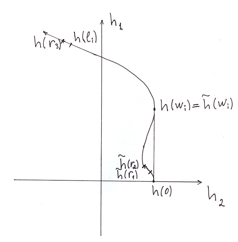
Figure 2: The case $h_{1}(l_{i})>0$

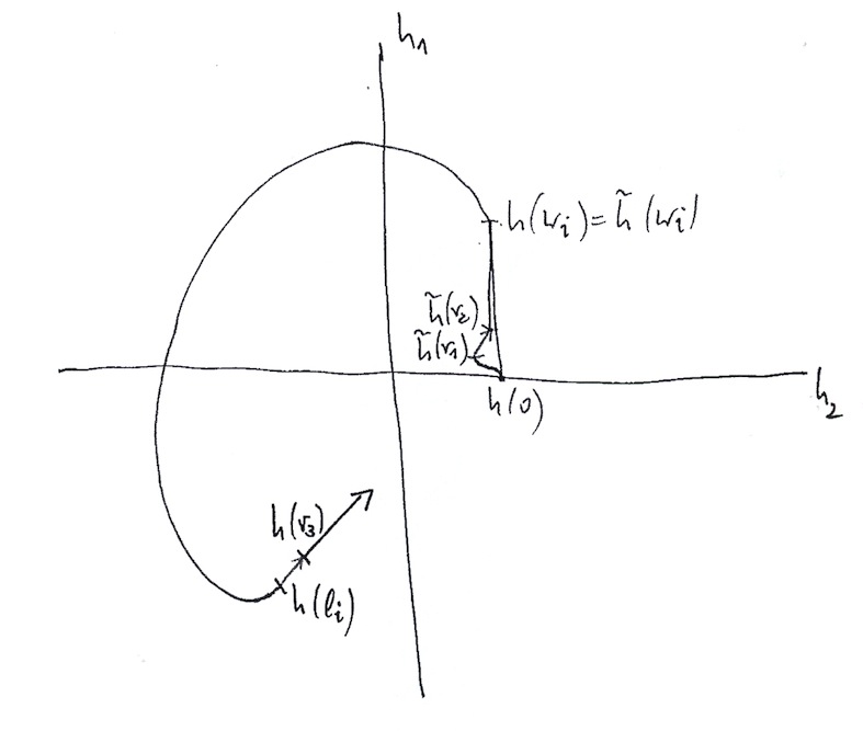
Figure 3: The case $h_{1}(l_{i})\leq 0$

The condition $h(r)=(r^{2},1)$ near $r=0$ means that near $L_{i}$ we have $\alpha=\alpha_{\rm st}$ with

$$\alpha_{\rm st}:=d\theta+r^{2}d\phi,$$

which extends smoothly over $r=0$. This gives us the desired extension of $\alpha_{h}$ from $K_{i}$ to $V_{i}$ and thus the extension of $\alpha$ from $N$ to $\bar{N}$. To get back to $N$ we just have to cut out the solid tori $\{r<l_{i}\}$.

Let $\xi:=\ker\alpha$ denote the contact structure defined by $\alpha$ on $\bar{N}$. An application of Corollary 3.1 to $(\bar{N},L:=\cup L_{i},n_{i},\alpha)$ gives us a new defining form $\beta$ for $\xi$ and an open book $(\bar{B},\bar{\pi})$ with the following properties. The contact form $\beta$ is supported by the open book $(\bar{B},\bar{\pi})$, and both the open book projection and the contact form restrict to a neighbourhood

$$W_{i}:=\{r\leq w_{i}\}$$

of $L_{i}$ in a standard way: $\bar{\pi}(r,\phi,\theta)=n_{i}\theta$ and $\beta=\alpha=\alpha_{\rm st}$.

Unfortunately, neither $\beta$ nor $\bar{\pi}$ is nice on $K_{i}$: It may even happen that the binding $\bar{B}$ intersects $K_{i}$, and the form $\beta$ need not be $T^{2}$-invariant on $K_{i}$. In order to take care of this, we introduce a new contact structure and new contact forms. We begin by picking a subdivision

Figure 4: The subdivision

$$0<r_{1}<r_{2}<w_{i}<l_{i}<r_{3}<R_{i}.$$ (14)

and an immersion $\tilde{h}:[0,w_{i}]\to{\mathbb{C}}$ with the following properties (see Figures 2, 3 and 4):

• $r_{2}-r_{1}=r_{3}-l_{i}$, or equivalently, $r_{3}-r_{2}=l_{i}-r_{1}=:l$;

• near $0$ and $w_{i}$ we have $\tilde{h}(r)=(r^{2},1)$;

• on $[r_{1},r_{2}]$ we have $\tilde{h}(r)=h(r+l)+(A,B)$ for some constant $(A,B)\in{\mathbb{C}}$;

• the function $\tilde{h}$ satisfies conditions (12) and (13).

Of course $r_{1},r_{2},r_{3},\tilde{h}$ depend on $i$, but we suppress this from the notation. We extend $\tilde{h}$ as $h$ over the interval $[w_{i},R]$. This defines a contact form $\alpha_{\tilde{h}}$ on each $V_{i}$ and thus a contact form $\tilde{\alpha}$ on $\tilde{N}$ which differs from $\alpha$ only on the neighbourhoods $W_{i}$. Recall that $\alpha$ and $\beta$ coincide on $W_{i}$, so we can define a contact form $\tilde{\beta}$ on $\bar{N}$ as $\tilde{\alpha}$ on each $W_{i}$ and as $\beta$ on the rest of $\bar{N}$. It is crucial to note that the $\tilde{h}_{1}^{\prime}>0$ implies that the contact form $\tilde{\beta}$ is supported by $(\bar{B},\bar{\pi})$. Note also that the contact forms $\tilde{\alpha}$ and $\tilde{\beta}$ define the same contact structure that we denote by $\tilde{\xi}$.

We introduce a third contact form defining $\tilde{\xi}$. For this, we introduce another subdivision point into subdivision (14), namely $r_{4}$:

$$0<r_{1}<r_{2}<w_{i}<l_{i}<r_{3}<r_{4}<R.$$

Now we pick a contact form $\beta^{\prime}$ defining $\tilde{\xi}$ that coincides with $\tilde{\alpha}$ on $\{r\in[0,r_{4}]\}$ and with $\beta=\tilde{\beta}$ on a neighbourhood of $\bar{N}\setminus(\cup V_{i})$.

We need one more ingredient: an isotopy of diffeomorphisms $\{\Phi_{t}\}_{t\in[0,1]}$ of the interval $[0,R]$ with the following properties (see Figure 5):

• $\Phi_{0}={{\mathchoice{\rm 1\mskip-4.0mul}{\rm 1\mskip-4.0mul}{\rm 1\mskip-4.5mul}{\rm 1\mskip-5.0mul}}}$;

• $\Phi_{t}={{\mathchoice{\rm 1\mskip-4.0mul}{\rm 1\mskip-4.0mul}{\rm 1\mskip-4.5mul}{\rm 1\mskip-5.0mul}}}$ near $0$ and $r_{4}$ for all $t\in[0,1]$;

• for $r\in[l_{i},r_{3}]$ we have $\Phi_{1}(r)=r-l$.

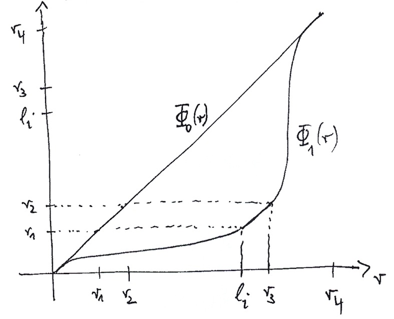
Figure 5: The diffeomorphism $\Phi$

For each $\Phi_{t}$ we also denote the induced radial diffeomorphism of $V_{i}$ by $\Phi_{t}$. This diffeomorphism extends from $\cup V_{i}$ to the rest of $\bar{N}$ by setting it to be the identity on the complement of $\cup V_{i}$. The resulting diffeomorphism will be denoted as $\Phi_{t}$ again. This finishes the necessary constructions and we now describe a homotopy of contact forms on $\bar{N}$ in 3 steps. The desired homotopy $\alpha_{t}$ will be obtained by restricting this homotopy to $N$.

Step 1. We start with the contact form $\tilde{\alpha}$ and linearly homotop it to $\beta^{\prime}$ (they define the same contact structure $\tilde{\xi}$). Since $\beta^{\prime}$ and $\tilde{\alpha}$ coincide on $\{r\leq r_{4}\}$, the homotopy is fixed there, in particular on $\{r\in[l_{i},r_{3}]\}$.

Step 2. We deform $\beta^{\prime}$ by setting $\beta_{t}^{\prime}:=\Phi_{t}^{*}\beta^{\prime}$. On $\{r\in[0,r_{4}]\}$ we have $\beta_{t}^{\prime}=\Phi_{t}^{*}\tilde{\alpha}=\Phi_{t}^{*}\alpha_{\tilde{h}}=\alpha_{\tilde{h}\circ\Phi_{t}}$. Since $\Phi_{t}={{\mathchoice{\rm 1\mskip-4.0mul}{\rm 1\mskip-4.0mul}{\rm 1\mskip-4.5mul}{\rm 1\mskip-5.0mul}}}$ near $0$ and $r_{4}$, the last equality is justified and we see that $\beta_{t}^{\prime}$ is $T^{2}$-invariant on $\{r\in[0,r_{4}]\}$ (so in particular on $\{r\in[l_{i},r_{3}]\}$) for all $t$.

Step 3. Finally, we deform $\Phi_{1}^{*}\beta^{\prime}$ by deforming $\beta^{\prime}$ to $\tilde{\beta}$. Namely, we consider the linear homotopy $(1-t)\beta^{\prime}+t\tilde{\beta}$ between the two forms $\beta^{\prime},\tilde{\beta}$ defining the contact structure $\tilde{\xi}$ and set

$$\beta_{t}:=\Phi_{1}^{*}\bigl{(}(1-t)\beta^{\prime}+t\tilde{\beta}\bigr{)}.$$

Note that on $\{r\in[0,w_{i}]\}$ we have

$$(1-t)\beta^{\prime}+t\tilde{\beta}=\alpha_{\tilde{h}}$$

and thus on $\{r\in[l_{i},r_{3}]\}$ we see that

$$\beta_{t}=\Phi_{1}^{*}\alpha_{\tilde{h}}=\alpha_{\tilde{h}\circ\Phi_{1}}=\alpha_{\tilde{h}(r-l)}=\alpha_{h(r)+(A,B)}=\alpha_{h}+A\,d\phi+B\,d\theta=\alpha+A\,d\phi+B\,d\theta$$

is fixed.

We define the homotopy $\alpha_{t}$ by restricting the homotopy constructed in Steps 1-3 above to $N$, thus $\alpha_{0}=\alpha$ and $\alpha_{1}=\Phi_{1}^{*}\tilde{\beta}|_{N}$. We define the open book decomposition $(B,\pi):=(\Phi_{1}^{-1}(\bar{B})|_{N},\bar{\pi}\circ\Phi_{1})$ on $N$. Now we check conditions (i-v) in the proposition with “$\{r\in[l_{i},r_{3}]\}$” in place of “near $\partial N$”.

(i) The contact form $\Phi_{1}^{*}\tilde{\beta}$ is supported by the open book $(\Phi_{1}^{-1}(\bar{B}),\bar{\pi}\circ\Phi_{1})$ because $\tilde{\beta}$ is supported by $(\bar{B},\bar{\pi})$. The last computation in Step 3 above shows that on $\{r\in[l_{i},r_{3}]\}$ we have $d\alpha_{1}=d\alpha_{h}=d\alpha$.

For (ii) note that $\bar{\pi}(\theta,r,\phi)=n_{i}\theta$ on $\{r\in[r_{1},r_{2}]\}$ implies that $\bar{\pi}\circ\Phi_{1}(\theta,r,\phi)=n_{i}\theta$ on $\{r\in[l_{i},r_{3}]\}$.

(iii) In the construction in Steps 1-3 above we always checked the $T^{2}$-invariance of the contact forms on $\{r\in[l_{i},r_{3}]\}$.

(iv) Recall that the homotopies in Steps 1 and 3 are constant near $T_{i}=\{r=l_{i}\}$, so the homotopy $\alpha_{t}$ is given near $T_{i}$ by the homotopy $\beta_{t}^{\prime}=\alpha_{h^{t}}$ in Step 2, where $h^{t}:=\tilde{h}\circ\Phi_{t}$. Thus for $t=1$ the first component satisfies $h^{1}_{1}(l_{i})=\tilde{h}_{1}(r_{1})>0$, and if $h_{1}(l_{i})>0$ then $h^{1}_{1}(l_{i})=\tilde{h}_{1}(r_{1})<\tilde{h}_{1}(l_{i})=h_{1}(l_{i})$ because we chose $\tilde{h}_{1}$ strictly increasing on $(0,l_{i}]$ in this case. Since $\Phi_{t}(l_{i})$ decreases from $l_{i}$ to $r_{1}$ as $t$ increases from $0$ to $1$, Figures 2 and 3 show that the derivatives $(h^{t})^{\prime}(l_{i})=\Phi_{t}^{\prime}(l_{i})\tilde{h}^{\prime}\bigl{(}\Phi_{t}(l_{i})\bigr{)}$ have rotation number $0$ if $h_{1}(l_{i})>0$ and $-1$ if $h_{1}(l_{i})<0$. Moreover, by adding positive rotations in the construction of $h$, we can decrease the rotation numbers by arbitrary integers, in particular we can make it $-1$ in the case $h_{1}(l_{i})>0$.

(v) can be arranged as in the special case discussed at the beginning of this proof. ∎

5 The structure theorem

In this section we collect and refine some results from [3] that will be needed in the proof in Section 6. Most importantly, we will use the following structure theorem.

Theorem 5.1.

Let $(\omega,\lambda)$ be a SHS on a closed $3$-manifold $M$ and set $f:=d\lambda/\omega$. Then there exists a (possibly disconnected and possibly with boundary) compact $3$-dimensional submanifold $N$ of $M$, invariant under the Reeb flow, a (possibly empty) disjoint union $U=U_{1}\cup\dots\cup U_{k}$ of compact integrable regions and a stabilizing 1-form $\tilde{\lambda}$ for $\omega$ with the following properties:

• ${\rm int\,}U\cup{\rm int\,}N=M$;

• the proportionality coefficient $\tilde{f}:=d\tilde{\lambda}/\omega$ is constant on each connected component of $N$;

• on each $U_{i}\cong[0,1]\times T^{2}$ the SHS $(\omega,\lambda)$ is $T^{2}$-invariant and $f(r,z)=\alpha_{i}r+\beta_{i}$ for constants $\alpha_{i}>0$, $\beta_{i}\in{\mathbb{R}}$;

• $\tilde{\lambda}$ is $C^{1}$-close to $\lambda$.

Moreover, if $\omega$ is exact we can arrange that $\tilde{f}$ attains only nonzero values on $N$.

We will also use the following result from [3].

Proposition 5.2.

Let $(\omega,\lambda)$ be a SHS on a closed $3$-manifold $M$ and set $f:=d\lambda/\omega$. Let $Z\subset{\mathbb{R}}$ be any set of Lebesgue measure zero containing a value $a\in Z\cap{\rm im}(f)$. Then there exists a stabilizing form $\tilde{\lambda}$ for $\omega$ such that $\tilde{f}:=d\tilde{\lambda}/\omega$ can be written as $\tilde{f}=\sigma\circ f$ for a function $\sigma:{\mathbb{R}}\to{\mathbb{R}}$ which is locally constant on a open neighbourhood of $Z$ (and thus $\tilde{f}$ is locally constant on an open neighbourhood of $f^{-1}(Z)$) and $\tilde{f}\equiv a$ on $f^{-1}(a)$. Moreover, for every $s\in[0,1)$ we can achieve that $\tilde{\lambda}$ is $C^{1+s}$-close to $\lambda$.

Using this, we now prove the following refinement of Theorem 5.1.

Corollary 5.3.

Every stable Hamiltonian structure on a closed 3-manifold $M$ is stably homotopic to a SHS $(\omega,\lambda)$ for which there exists a (possibly disconnected and possibly with boundary) compact $3$-dimensional submanifold $N=N^{+}\cup N^{-}\cup N^{0}$ of $M$, invariant under the Reeb flow, and a (possibly empty) disjoint union $U=U_{1}\cup\dots\cup U_{k}$ of compact integrable regions with the following properties:

• ${\rm int\,}U\cup{\rm int\,}N=M$;

• the proportionality coefficient $f:=d\lambda/\omega$ is constant positive resp. negative on each connected component of $N^{+}$ resp. $N^{-}$;

• on each $U_{i}\cong[0,1]\times T^{2}$ the SHS $(\omega,\lambda)$ is $T^{2}$-invariant and $f$ is nowhere zero;

• on $N^{0}$ there exists a closed $1$-form $\bar{\lambda}$ representing a primitive integer cohomology class $\bar{\lambda}\in H^{1}(N^{0};{\mathbb{Z}})$ such that $\bar{\lambda}\wedge\omega>0$ and $\bar{\lambda}$ is $T^{2}$-invariant near $\partial N^{0}$.

Proof.

Consider a SHS $(\omega,\lambda)$ and apply the Structure Theorem 5.1 to find a new stabilizing 1-form $\tilde{\lambda}$. Denote by $N^{+},N^{0},N^{-}$ the union of components of $N$ on which $\tilde{f}=d\tilde{\lambda}/\omega$ is positive (resp. zero, negative). If the original proportionality coefficient $f=d\lambda/\omega$ is nowhere zero, then we may assume that the new proportionality coefficient $\tilde{f}$ is nowhere zero and $(\omega,\tilde{\lambda})$ has all the desired properties (with $N^{0}=\emptyset$). So suppose that $f$ has nonempty zero set $f^{-1}(0)$. The proof of Theorem 5.1 (using Proposition 5.2 with $Z$ the set of critical values together with the value $a=0$) allows us to arrange that $f^{-1}(0)$ is contained in the interior of the flat part $N^{0}$.

The new stabilizing form $\tilde{\lambda}$ restricts as a closed form to $N^{0}$. We $C^{1}$-perturb $\tilde{\lambda}|_{N^{0}}$ to get a $1$-form $\hat{\lambda}$ on $N^{0}$ representing a rational cohomology class. Let $V\cong[0,1]\times T^{2}\subset N^{0}$ be a part of an integrable region sitting in $N^{0}$ as a collar neighbourhood of one of its boundary components $\{1\}\times T^{2}$. Since the restriction $\tilde{\lambda}|_{V}$ is $T^{2}$-invariant and $\hat{\lambda}$ is $C^{1}$-close to $\tilde{\lambda}$, the $T^{2}$ average $\lambda_{inv}$ of $\hat{\lambda}$ on $V$ is $C^{1}$-close to $\hat{\lambda}$. As $\lambda_{inv}$ and $\hat{\lambda}$ represent the same cohomology class on $V$, we can write $\hat{\lambda}=\lambda_{inv}+d\chi$ for a smooth function $\chi$ on $V$. Moreover, $C^{1}$-closeness of $\lambda_{inv}$ and $\hat{\lambda}$ allows us to choose $\chi$ also $C^{1}$-small. Let $\rho$ be a cutoff function on $[0,1]$ which equals $1$ near $0$ and $0$ near $1$. Set $\bar{\lambda}:=\lambda_{inv}+d(\rho\chi)$ on $V$ and extend this form as $\hat{\lambda}$ inside $N^{0}$. The closed form $\bar{\lambda}$ is $T^{2}$-invariant near the boundary of $N^{0}$. Note also that

$$\bar{\lambda}-\hat{\lambda}=\lambda_{inv}+d(\rho\chi)-(\lambda_{inv}+d\chi)=d(\rho\chi)-d\chi=d(\chi(\rho-1))$$

on $V$. Therefore, the difference $\bar{\lambda}-\hat{\lambda}$ is exact on $N^{0}$ and thus $\bar{\lambda}$ represents a rational cohomology class. Assume the procedure above has been performed near all boundary components of $N^{0}$. Now $C^{1}$-smallness of $\chi$ implies $C^{1}$-smallness of $\rho\chi$. This together with the computation above and the $C^{1}$-smallness of the difference $\hat{\lambda}-\tilde{\lambda}$ ensures that $\bar{\lambda}\wedge\omega>0$ on $N^{0}$. After multiplying $\bar{\lambda}$ with a rational number we may assume that it represents a primitive integer cohomology class in $H^{1}(N^{0},{\mathbb{Z}})$.

The set $N^{0}$ and the $1$-form $\bar{\lambda}$ on it have the desired properties. However, the new proportionality coefficient $\tilde{f}$ may still vanish on some integrable region $U_{i}$. To remedy this, we choose $\delta>0$ so small that $\{f<\delta\}\subset N^{0}$. Now we apply Theorem 5.1 again to the original SHS $(\omega,\lambda)$ to obtain new $\tilde{\lambda},\tilde{f}$ and new regions $\tilde{N}^{\pm},\tilde{N}^{0},\tilde{U}_{i}$. Moreover, we can make $\|\tilde{\lambda}-\lambda\|_{C^{1}}$ so small that $\tilde{N}^{0}\subset\{\tilde{f}=0\}\subset\{f<\delta\}\subset N^{0}$. In particular, $\tilde{f}$ does not vanish on a neighbourhod $W$ of $M\setminus{\rm int\,}N^{0}$. Now the SHS $(\omega,\tilde{\lambda})$, the old set $N^{0}$ and 1-form $\bar{\lambda}$, and the intersections of the new sets $\tilde{U}_{i}$ and $\tilde{N}^{\pm}$ with $W$ satisfy all conditions in Corollary 5.3. ∎

Remark 5.4.

If $f$ is non-negative, then so is the new proportionality coefficient constructed in the proof of Corollary 5.3 and hence $N^{-}=\emptyset$. Then all binding components of the open book constructed in the proof of Theorem 1.1 in the next section occur in $N^{+}$ and thus have positive signs.

6 Proof of the main theorem

In this section we prove Theorem 1.1.

We will need two more technical results. As before, we consider $[a,b]\times T^{2}$ with cordinates $(r,\phi,\theta)$. For functions $h=(h_{1},h_{2}):[a,b]\to{\mathbb{C}}$ and $g=(g_{1},g_{2}):[a,b]\to{\mathbb{C}}$ we define 1-forms

$$\alpha_{h}=h_{1}(r)d\phi+h_{2}(r)d\theta,\qquad\lambda_{g}=g_{1}(r)d\phi+g_{2}(r)d\theta.$$

Then $(d\alpha_{h},\lambda_{g})$ is a SHS iff

$$\langle g^{\prime},ih^{\prime}\rangle=0,\qquad\langle g,ih^{\prime}\rangle>0.$$ (15)

The following result is proved in [3].

Proposition 6.1.

Let $h_{t}:[0,1]\to{\mathbb{C}}$, $t\in[a,b]$ be a homotopy of immersions such that for each $t$ the slope $h_{t}^{\prime}/|h_{t}^{\prime}|$ restricted to $[\varepsilon,1-\varepsilon]$ is nonconstant. Let $\bar{g}_{t}:[0,\varepsilon]\cup[1-\varepsilon,1]$, $t\in[a,b]$ be a homotopy such that $(h_{t},\bar{g}_{t})$ satisfies (15) on $[0,\varepsilon]\cup[1-\varepsilon,1]$ for all $t\in[a,b]$. Then there exists a homotopy $g_{t}$ which agrees with $\bar{g}_{t}$ to $[0,\varepsilon]\cup[1-\varepsilon,1]$ such that $(h_{t},g_{t})$ satisfies (15) on $[0,1]$ for all $t\in[a,b]$.

Finally, we will need the following simple lemma on immersions. Recall that $\alpha_{h}$ is a positive contact form iff

$$h_{1}^{\prime}h_{2}-h_{2}^{\prime}h_{1}>0.$$ (16)

Lemma 6.2.

Let $h=(h_{1},h_{2}):[-\delta,\delta]\to{\mathbb{C}}$ be an immersion satisfying the contact condition (16) and $h_{1}^{\prime}>0$. Then:

(a) For any constant $B\geq 0$ the immersion $h+(0,B)$ satisfies (16).

(b) If in addition $h_{2}(0)>0$, then for every $\varepsilon>0$ there exists a constant $A\in{\mathbb{R}}$ such that for all $t\in[0,1]$ the immersion $h+t(A,0)$ satisfies (16) near $r=0$, and $(h_{1}+A)(0)\in(0,\varepsilon)$.

Proof.

(a) Condition (16), $h_{1}^{\prime}>0$ and $B\geq 0$ imply

$$h_{1}^{\prime}(h_{2}+B)-h_{2}^{\prime}h_{1}=(h_{1}^{\prime}h_{2}-h_{2}^{\prime}h_{1})+h_{1}^{\prime}B>0.$$

(b) At $r>0$ we have $h_{1}^{\prime}h_{2}>0$ by assumption, so for sufficiently small $\delta\in(0,\varepsilon)$

$$0<h_{1}^{\prime}h_{2}-h_{2}^{\prime}\delta=h_{1}^{\prime}h_{2}-h_{2}^{\prime}(h_{1}+A)$$

with $A:=\delta-h_{1}(0)$. Linear interpolation from the right hand side to
$h_{1}^{\prime}h_{2}-h_{2}^{\prime}h_{1}>0$ yields $h_{1}^{\prime}h_{2}-h_{2}^{\prime}(h_{1}+tA)>0$ for all $t\in[0,1]$. ∎

After these preparations, we now turn to the

Proof of Theorem 1.1.

Let $(\omega,\lambda)$ be a SHS obtained after application of Corollary 5.3. We will use the following terminology: $N^{\pm}$ and $N^{0}$ are called positive/negative contact parts and the flat parts; connected components of $N^{\pm}$ and $N^{0}$ will be called regions. We will construct the stable homotopy and the supporting open book successively on the different types of regions.

Flat regions. Consider a flat region $N$ with the primitive integer $1$-form $\bar{\lambda}$ provided by Corollary 5.3. Integration of $\bar{\lambda}$ over paths from a fixed base point yields a fibration

$$\pi:N\to S^{1}$$ (17)

such that $d\pi=\bar{\lambda}|_{N}$. Let $k_{i}\gamma_{i}$ denote the restriction of the cohomology class $[\bar{\lambda}|_{N}]$ to the boundary component $T_{i}$ of $N$, where $\gamma_{i}\in H^{1}(T_{i};{\mathbb{Z}})$ is a primitive integer cohomology class and $k_{i}\in{\mathbb{N}}$ is the multiplicity. Since $\bar{\lambda}$ is $T^{2}$-invariant near $T_{i}$, there exist coordinates near $T_{i}$ in which the projection is given by $\pi(r,\phi,\theta)=k_{i}\theta$.

Contact regions. Now let $N$ be a contact region, so $\omega=c\,d\lambda$ on $N$ for some constant $c\neq 0$. After possibly switching the orientation of $N$, we may assume that $\lambda$ is a positive contact form (but $c$ may still be negative). Let $[-\delta,\delta]\times T^{2}$ be a tubular neighbourhood of a boundary component $T_{i}=\{0\}\times T^{2}$ of $N$ which is contained in an integrable region (such that $[0,\delta]\times T^{2}\subset N$). On this neighbourhood the SHS $(\omega,\lambda)$ is given by $(c\,d\alpha_{h},\alpha_{h})$ for some immersion $h:[-\delta,\delta]\to{\mathbb{C}}$ satisfying the contact condition (12). After a perturbation of $h$ supported near $r=0$ we may assume that the cohomology class $[\alpha_{h}|_{T_{i}}]\in H^{1}(T_{i};{\mathbb{R}})$ is rational. Let $\gamma_{i}$ be the primitive integer cohomology class in $H^{1}(T_{i};{\mathbb{Z}})$ positively proportional to $[\alpha_{h}|_{T_{i}}]$. We choose linear coordinates $(\phi,\theta)$ on $T^{2}$ in which $\gamma_{i}=[d\theta]$. Then the positive contact condition yields $d\theta\wedge d\alpha_{h}>0$ near $r=0$. Since $\alpha_{h}=h_{1}(r)d\phi+h_{2}(r)d\theta$, the immersion $h=(h_{1},h_{2})$ satisfies $h_{1}(0)=0$, $h_{1}^{\prime}(0)>0$, and $h_{2}(0)>0$. So after a perturbation of $h$ supported near $r=0$ we may assume that $h=(r,a)$ near $r=0$ with a constant $a>0$. By a further deformation (keeping the contact condition) supported near $r=0$ we can achieve that $h=(r,1)$ near $r=0$. After performing these deformations near all boundary components of $N$, we can apply the easy case of Proposition 4.1 in which condition (v) (with $l_{i}=0$) holds near all boundary components. It yields a homotopy of positive contact forms $\lambda_{t}$ on $N$ such that $\lambda_{t}=\lambda$ near $\partial N$, and $\lambda_{1}$ is supported by an open book $(B,\pi)$ with $\pi(r,\phi,\theta)=n_{i}\theta$ near each boundary component $T_{i}$. We obtain a corresponding stable homotopy $(\omega_{t},\lambda_{t})$ by setting $\omega_{t}:=c\,d\lambda_{t}$ with the constant $c\neq 0$ from above.

Introducing small contact regions. It remains to consider an integrable region $[a,b]\times T^{2}$. The open book projections on the adjacent contact/flat regions constructed above provide primitive integer cohomology classes $\gamma_{a}\in H^{1}(T^{2},{\mathbb{Z}})$ near $a$ and $\gamma_{b}\in H^{1}(T^{2},{\mathbb{Z}})$ near $b$. Note that in general we will have $\gamma_{a}\neq\gamma_{b}$, in which case the open book projections $\pi$ given near the boundary of $[a,b]\times T^{2}$ do not extend over $[a,b]\times T^{2}$. To deal with this, we choose a subdivision

$$a=r_{0}<r_{1}<\dots<r_{n}=b$$ (18)

and a sequence $\{\gamma_{k}\}_{k=1,\dots,n}$ of primitive integer cohomology classes in $H^{1}(T^{2},{\mathbb{Z}})$ with the following properties:

• $\gamma_{1}=\gamma_{a}$ and $\gamma_{n}=\gamma_{b}$;

• on the interval $[r_{k-1},r_{k}]$ ($k=1,\dots,n$) we have $\bar{\gamma}_{k}\wedge\omega>0$, where $\bar{\gamma}_{k}=p_{k}d\phi+q_{k}d\theta$ is the $T^{2}$-invariant representative of $\gamma_{k}$.

Recall that, according to Corollary 5.3, the proportionality factor $f=d\lambda/\omega$ is nowhere zero on $[a,b]\times T^{2}$. We apply Proposition 5.2 (with $Z=\{a\}=\{a_{k}\}$ and followed by averaging) to the level sets $a_{k}=f(r_{k})$, $k=1,...,n-1$, to find a new $T^{2}$-invariant stabilizing 1-form $\tilde{\lambda}$ for $\omega$ such that $\tilde{f}:=d\tilde{\lambda}/\omega$ satisfies $\tilde{f}(r)\equiv a_{k}\neq 0$ on some intervals $[r_{k}-\delta_{k},r_{k}+\delta_{k}]$. We rename $\tilde{\lambda},\tilde{f}$ back to $\lambda,f$. We will refer to the regions $\{r\in[r_{k}-\delta_{k},r_{k}+\delta_{k}]$ as small contact regions in order to distinguish them from the original (large) contact or flat regions constructed above. It is important to note that adjacent small contact regions have the same sign, i.e. the contact structures are either both positive or both negative.

We apply Proposition 4.1 to construct contact homotopies and suporting open books on the small contact regions. To extend them over the integrable regions $[r_{k-1},r_{k}]\times T^{2}$, we distinguish two cases: integrable regions $[a,r_{1}]\times T^{2}$ and $[r_{n-1},b]\times T^{2}$ connect a large contact/flat region to a small contact region, and regions $[r_{k-1},r_{k}]\times T^{2}$, $k=2,...,n-1$, connecting two small contact regions. Recall that on each such region we have $\bar{\gamma}_{k}\wedge\omega>0$ for some $T^{2}$-invariant 1-form on $T^{2}$ representing a primitive integer cohomology class. After a linear change of coordinates we may assume that $\bar{\gamma}_{k}=d\theta$ and thus

$$d\theta\wedge\omega>0.$$

Integrable regions I. Consider an integrable region $[a,r_{1}]\times T^{2}$ connecting a large contact/flat region $N$ with a small contact region $[r_{1}-\delta,r_{1}+\delta]\times T^{2}$. (The region $[r_{n-1},b]\times T^{2}$ can be treated analogously).

In both the contact and flat case, the stable homotopy on $N$ constructed above was constant near $\{r=a\}$. So in order to extend the homotopy over $[a,r_{1}]$ we need to arrange rotation number zero at $r=r_{1}-\delta$ in the application of Proposition 4.1 to the small contact region. To achieve this, we prepare the stabilizing 1-form $\lambda$ before applying Proposition 4.1.

We write $\omega=d\alpha_{h}$ and $\lambda=\lambda_{g}$ for an functions $h=(h_{1},h_{2}):[a,b]\to{\mathbb{C}}$ and $g=(g_{1},g_{2}):[a,b]\to{\mathbb{C}}$ satisfying (15). We may assume that $\lambda$ is a positive contact form on $[r_{1}-\delta,r_{1}+\delta]\times T^{2}$. (Otherwise we make the orientation reversing coordinate change $\Psi:\phi\mapsto-\phi$ and replace $(\omega,\lambda)$ by $(-\Psi^{*}\omega,\Psi^{*}\lambda)$). So we have $h(r)-cg(r)\equiv{\rm const}\in{\mathbb{C}}$ on $[r_{1}-\delta,r_{1}+\delta]$ for some $c>0$.

Fix some $\varepsilon>0$ that will be specified later. We choose $B\geq 0$ such that $g_{2}(0)+B>0$. By Lemma 6.2 (a) the homotopy $\{g+t(0,B)\}_{t\in[0,1]}$ satisfies the contact condition on $[r_{1}-\delta,r_{1}+\delta]$. By Lemma 6.2 (b) we find $A\in{\mathbb{R}}$ and a homotopy $\{g+(0,B)+t(A,0)\}_{t\in[0,1]}$ of contact immersions on $[r_{1}-\delta,r_{1}+\delta]$ (for a possibly smaller $\delta$) such that $(g_{1}+A)(r)\in(0,\varepsilon)$ for all $r$. Denote by $g^{t}$, $t\in[0,1]$, the concatenation of these two contact homotopies on $[r_{1}-\delta,r_{1}+\delta]$ and note that $c(g^{t})^{\prime}=h^{\prime}$ for all $t$, so the $g^{t}$ satisfy (15) for all $t$. We use Proposition 6.1 to extend this homotopy to $[a,b]$ such that it satisfies (15) and coincides with $g$ outside a neighbourhood of $[r_{1}-\delta,r_{1}+\delta]$. We rename the new stabilizing function $g^{1}$ back to $g$, so we have achieved that $g$ is a contact immersion on $[r_{1}-\delta,r_{1}+\delta]$ with first component $g_{1}\in(0,\varepsilon)$. Moreover, we still have $h(r)-cg(r)\equiv{\rm const}\in{\mathbb{C}}$ on $[r_{1}-\delta,r_{1}+\delta]$ with $c>0$ as above. (Note that we may have destroyed positivity of $f=d\lambda/\omega$, but we will not need this any more).

Now we apply Proposition 4.1 to the small contact region $(N,\alpha)=([r_{1}-\delta,r_{1}+\delta]\times T^{2},\lambda_{g})$ to find an open book decomposition $(B,\pi)$ and a contact homotopy $\lambda_{t}$. Write $\lambda_{t}=\lambda_{g^{t}}$ near the boundary torus $T_{i}=\{r_{1}-\delta\}\times T^{2}$. Proposition 4.1 (iv) (with $h^{t}=g^{t}$ and $l_{i}=r_{1}-\delta$) and $g_{1}\in(0,\varepsilon)$ implies that the first component of $g^{1}$ satisfies $g^{1}_{1}\in(0,\varepsilon)$. Moreover, we can choose $(g^{t})^{\prime}(r_{1}-\delta)$, $t\in[0,1]$, to have rotation number zero.

We extend $\lambda_{t}$ to a stable homotopy $(\omega_{t},\lambda_{t})$ on $[r_{1}-\delta,r_{1}+\delta]\times T^{2}$ by $\omega_{t}:=cd\lambda_{t}$. Near $r=r_{1}-\delta$ we have $\omega_{t}=\omega_{h^{t}}$ with immersions $h^{t}$, $t\in[0,1]$, defined by $h^{t}(r)-cg^{t}(r)\equiv{\rm const}\in{\mathbb{C}}$. Thus the first components satisfy $|h_{1}^{1}-h_{1}|=c|g_{1}^{1}-g_{1}|<c\varepsilon$ near $r=r_{1}-\delta$. Since $h_{1}^{\prime}>0$ on $[a,r_{1}]$, for sufficiently small $\varepsilon$ we can extend $h^{1}$ from a neighbourhood of $r_{1}-\delta$ to an immersion on $[a,r_{1}-\delta]$ which coincides with $h$ near $r=a$ and whose first component satisfies $(h_{1}^{1})^{\prime}>0$ everywhere. Moreover, since $(h^{t})^{\prime}(r_{1}-\delta)$, $t\in[0,1]$, has rotation number zero, we can extend the $h^{t}$ from a neighbourhood of $r_{1}-\delta$ to immersions on $[a,r_{1}-\delta]$ which coincide with $h$ near $r=a$ and satisfy $h^{0}=h$. Now we use Proposition 6.1 to extend the $g^{t}$ from a neighbourhood of $r_{1}-\delta$ to functions on $[a,r_{1}-\delta]$ which coincide with $g$ near $r=a$ such that $g^{0}=g$ and $(h^{t},g^{t})$ satisfies (15) for all $t\in[0,1]$. Thus $(\omega_{t},\lambda_{t})=(d\alpha_{h^{t}},\lambda_{g^{t}})$ is a stable homotopy on $[a,r_{1}-\delta]\times T^{2}$, which coincides with the previously constructed homotopies near the boundary, from $(\omega_{0},\lambda_{0})=(\omega,\lambda)$ to $(\omega_{1},\lambda_{1})$ satisfying $d\theta\wedge\omega_{1}>0$.

Integrable regions II. It remains to consider an integrable region $[r_{k-1},r_{k}]\times T^{2}$ connecting two small contact regions. Recall that the two contact regions have the same sign, so we may assume that they are both positive. (Otherwise we make the orientation reversing coordinate change $\Psi:\phi\mapsto-\phi$ and replace $(\omega,\lambda)$ by $(-\Psi^{*}\omega,\Psi^{*}\lambda)$).

Let us ignore for the moment the cohomology classes of $\omega_{t}$, which we will discuss below. Then we conclude the argument as follows. We apply Proposition 4.1 to both small contact regions, choosing the option “rotation number $-1$” in Proposition 4.1 (iv) at both boundary tori $T_{k-1}=\{r_{k-1}+\delta\}\times T^{2}$ and $T_{k}=\{r_{k}-\delta\}\times T^{2}$. Note that the chosen coordinates $(r,\phi,\theta)$ on $[r_{k-1},r_{k}]\times T^{2}$ are related to the coordinates in Proposition 4.1 by the identity map near $T_{k-1}$, and (for example) by the map $(r,\phi,\theta)\mapsto(-r,-\phi,\theta)$ near $T_{k}$. Thus, in the integrable region coordinates $(r,\phi,\theta)$ the rotation number equals $-1$ at $T_{k-1}$ and $+1$ at $T_{k}$. (Here it is crucial that no positive and negative contact regions are connected by an integrable region!). Thus, the homotopy of Hamiltonian structures $\omega_{t}$ given on the small contact regions extends over the region $[r_{k-1},r_{k}]\times T^{2}$ (by extending the corresponding immersions $h^{t}$) such that $\omega_{0}=\omega_{1}=\omega$. We use Proposition 6.1 extend the $\lambda_{t}$ from the contact regions to stabilizing 1-forms over $[r_{k-1},r_{k}]\times T^{2}$. Note that $d\theta\wedge\omega_{1}=d\theta\wedge\omega_{0}>0$ on $[r_{k-1},r_{k}]\times T^{2}$.

Defining the open book. The preceding step finishes the construction of the homotopy of SHS $(\omega_{t},\lambda_{t})$, $t\in[0,1]$, on $M$. It remains to define the open book $(B,\pi)$ supporting $(\omega_{1},\lambda_{1})$. For this, recall that in Proposition 4.1 (ii) we have the freedom to prescribe the multiplicities $n_{i}\geq K$ of the open book projection near each boundary component $T_{i}$ of a contact region, for some constant $K$ depending on this region. Let $K_{0}$ be the maximum of these constants $K$ over all (large and small) contact regions. We set the multiplicities at all boundary tori of contact regions equal to $K_{0}$, except for those adjacent to flat regions. For the latter the choice can be made as follows. Let $[a,b]\times T^{2}$ be an integrable region with $T_{a}=\{a\}\times T^{2}$ contained in a flat region $N$ and $\{b\}\times T^{2}$ in a (small) contact region $N^{c}$ (the opposite case is analogous). By the discussion following equation (17), there is a primitive cohomology class $\gamma_{a}\in H^{1}(T_{a};{\mathbb{Z}})$ and a multiplicity $k_{a}\in{\mathbb{N}}$ such that $k_{a}l_{a}=[d\pi|_{T_{a}}]$ for the projection $\pi:N\to S^{1}$. We choose the multiplicity for $T_{b}$ in Proposition 4.1 to be the product $k_{a}K_{0}$. Then the fibration $K_{0}\pi:N\to S^{1}={\mathbb{R}}/{\mathbb{Z}}$ extends over the integrable region and coincides with the one produced by Proposition 4.1 near $T_{b}$. With these choices, the open book projections on the contact regions and the projections on the flat regions extend over all the integrable regions to an open book structure on $M$ supporting $(\omega_{1},\lambda_{1})$.

Preserving the cohomology class. The discussion so far finishes the proof of Theorem 1.1 except for vanishing of the cohomology classes $[\omega_{t}-\omega]\in H^{2}(M;{\mathbb{R}})$. Let us analyze how we can ensure exactness in the previous constructions. On a flat region we have $\omega_{t}=\omega$. On a (large or small) contact region $N$ we have $\omega=c\,d\lambda$ for some constant $c\neq 0$. We change $\lambda$ by a contact homotopy $\lambda_{t}$ and define $\omega_{t}$ by $\omega_{t}=c\,d\lambda_{t}$. Next consider an integrable region $U=[a,b]\times T^{2}$ connecting two contact/flat regions $N_{0},N_{\ell}$ on which $\omega=c_{i}d\lambda$ for constants $c_{0},c_{\ell}\neq 0$. Moreover, suppose that we have several small integrable regions $N_{i}=[r_{i}-\delta,r_{i}+\delta]\times T^{2}$ in $U$ on which $\omega=c_{i}d\lambda$ for constants $c_{i}\neq 0$, $i=1,\dots,\ell-1$. We change $\lambda$ by a contact homotopy $\lambda_{t}$ and define $\omega_{t}$ by $\omega_{t}=c_{i}d\lambda_{t}$ on each $N_{i}$, $i=0,\dots,\ell$. Denote by $\partial^{\pm}N_{i}=\{r_{i}\pm\delta\}\times T^{2}$ the left resp. right boundary components for $i=1,\dots,\ell-1$ and set $\partial^{+}N_{0}=\{a\}\times T^{2}$, $\partial^{-}N_{\ell}=\{b\}\times T^{2}$. On $U$ we can write $\lambda=\lambda_{g}$ and $\omega=d\alpha_{h}$ for functions $g,h:[a,b]\to{\mathbb{C}}$ satisfying (15). So near each boundary component $\partial^{\pm}N_{i}$ we have a relation

$$h-c_{i}g=k_{i}^{\pm}$$ (19)

for some constants $k_{i}^{\pm}\in{\mathbb{C}}$. Moreover, near $\partial^{\pm}N_{i}$ we can write $\lambda_{t}=\lambda_{g^{t}}$ for locally defined functions $g^{t}$. Now suppose that we find a family of immersions $h^{t}:[a,b]\to{\mathbb{C}}$ and a family of constants $k^{t}\in{\mathbb{C}}$ such that $h^{0}=h$, $k^{0}=0$ and

$$h^{t}=\begin{cases}c_{i}g^{t}+k_{i}^{\pm}&\text{ near }r=r_{i}\pm\delta\\ c_{0}g^{t}+k_{0}^{+}+k^{t}&\text{ near }r=a\\ c_{\ell}g^{t}+k_{\ell}^{-}+k^{t}&\text{ near }r=b.\end{cases}$$ (20)

Then we obtain an exact homotopy of HS $\omega_{t}=\omega+d\beta_{t}$ on $U$, extending the given one on $\cup_{i}N_{i}$ and $T^{2}$-invariant on $\cup_{i}N_{i}$, by setting

$$\beta_{t}:=\begin{cases}c_{0}(\lambda_{t}-\lambda)&\text{ on }N_{0}\\ c_{\ell}(\lambda_{t}-\lambda)&\text{ on }N_{\ell}\\ c_{i}(\lambda_{t}-\lambda)-\alpha_{k^{t}}&\text{ on }N_{i},\ i=1,\dots,\ell-1\\ \alpha_{h^{t}}-\alpha_{h}-\alpha_{k^{t}}&\text{ on }U\setminus\cup_{i}N_{i}.\end{cases}$$

Finally, Proposition 6.1 provides a homotopy of stabilizing 1-forms $\lambda_{t}$ for $\omega_{t}$ on $U$, extending the given one on $\cup_{i}N_{i}$ and $T^{2}$-invariant on $\cup_{i}N_{i}$. Note that in “Integrable regions I” above we arranged condition (20) with constant $k^{t}=0$, but in “Integrable regions II” this will in general fail.

The $\theta$ – $\phi$ – $\theta$ trick. Consider again an integrable region $[a,b]\times T^{2}$ connecting two (small) positive contact regions $N_{a},N_{b}$ with a SHS $(\omega,\lambda)=(d\alpha_{h},\lambda_{g})$ satisfying $d\theta\wedge\omega>0$, i.e. $h_{1}^{\prime}>0$. Near $r=a,b$ we are given a contact homotopy $\lambda_{t}$ and define $\omega_{t}$ by $\omega_{t}=c_{a}d\lambda_{t}$ resp. $\omega_{t}=c_{b}d\lambda_{t}$, i.e.

$$h(r)-c_{a}g(r)=k_{a}\text{ resp. }h(r)-c_{b}g(r)=k_{b}$$

for constant $c_{a},c_{b}>0$ and $k_{a},k_{b}\in{\mathbb{C}}$. We face the following problem: In order to ensure exactness we wish to define the homotopy $h^{t}:[a,b]\to{\mathbb{C}}$ satisfying (20) near $r=a,b$, but then the difference of the first components of $h^{1}(b)-h^{1}(a)=c_{b}g^{1}(b)+k_{b}-c_{a}g^{1}(a)-k_{a}$ may be negative and we cannot achieve $(h^{1}_{1})^{\prime}>0$. To overcome this problem, we introduce two new small contact regions $N_{x}=[x-\delta,x+\delta]\times T^{2}$ and $N_{y}=[x-\delta,y+\delta]\times T^{2}$ around new subdivision points $x$ and $y$:

$$a<x<y<b.$$

Now we repeat the construction using the following open book projections:

$$\pi(r,\phi,\theta):=\begin{cases}\theta&\text{ on }[a,x-\delta]\\ \phi&\text{ on }[x+\delta,y-\delta]\\ \theta&\text{ on }[y+\delta,b].\end{cases}$$ (21)

It will turn out that, with this trick, we can use the freedom in Proposition 4.1 and Lemma 6.2 to achieve exactness of $[\omega_{t}-\omega]$ as well as positivity of $d\theta\wedge\omega_{1}$ resp. $d\phi\wedge\omega_{1}$ on the respective regions. This will be carried out in the remaining two steps.

Preparation for the exact homotopy. We first homotop the immersion $h:[a,b]\to{\mathbb{C}}$ through immersions rel $\partial[a,b]$ to one (still denoted by $h$) which satisfies

$$h(r)=e^{-i(r-x+\pi/4)}$$

on some small subinterval $[x-\delta,y+\delta]\subset(a,b)$, see Figure 6.

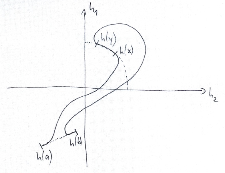
Figure 6: The deformation of $h$

Hence $h|_{[x-\delta,y+\delta]}$ is contact and satisfies the conditions

$$\hat{h}_{1}^{\prime}>0,\qquad\hat{h}_{2}^{\prime}<0,\qquad ih^{\prime}=h.$$

Note that we may have lost the condition $(h_{1})^{\prime}>0$ outside the interval
$[x-\delta,y+\delta]$. The 1-form $h_{1}(r)d\phi+h_{2}(r)d\theta$ stabilizes $d\alpha_{h}$ on $[x-\delta,y+\delta]$. So by Proposition 6.1 we find a stabilizing form $\lambda_{g}$ for $\omega=d\alpha_{h}$ on $[a,b]\times T^{2}$ which agrees with the original $\lambda$ near the boundary and such that $g=h$ on $[x-\delta,y+\delta]$.

Next we use Lemma 6.2 and Proposition 6.1 to modify the stabilizing 1-form $\lambda_{g}$ on the small contact regions $N_{x}=[x-\delta,x+\delta]\times T^{2}$ and $N_{y}=[y-\delta,y+\delta]\times T^{2}$ (possibly shrinking $\delta$ in the process). For this, we make the following orientation preserving coordinate change on $[x-\delta,y+\delta]\times T^{2}$:

$$\hat{\theta}:=\phi,\quad\hat{\phi}:=-\theta.$$

We rewrite $\lambda_{g}$ in the new coordinates,

$$\lambda_{g}=g_{1}d\phi+g_{2}d\theta=\hat{g}_{1}d\hat{\phi}+\hat{g}_{2}d\hat{\theta},\qquad\hat{g}_{1}=-g_{2},\quad\hat{g}_{2}=g_{1}$$

and note that the contact condition $\langle ig^{\prime},g\rangle>0$ is preserved by this coordinate change. Moreover, by construction we have $(\hat{g}_{1})^{\prime}=-g_{2}^{\prime}=-h_{2}^{\prime}>0$. Thus, by Lemma 6.2 (applied in the coordinates $(\hat{\phi},\hat{\theta})$ near $x$ and $y$) and Proposition 6.1, we can add complex constants to $g$ near $x,y$ to obtain a new stabilizing form, still denoted by $\lambda_{g}$, which coincides with the previous one outside a neighbourhood of $N_{x}\cup N_{y}$ and satisfies

$$\begin{cases}0<\hat{g}_{1}<\varepsilon\text{ and }g_{1}=\hat{g}_{2}>0&\text{ on }[x-\delta,x+\delta],\\ 0<\hat{g}_{1}<\varepsilon\text{ and }g_{1}=\hat{g}_{2}\geq A>0&\text{ on }[y-\delta,y+\delta]\end{cases}$$ (22)

for an arbitrarily small constant $\varepsilon$ and an arbitrarily large constant $A$ that will be specified later.

Constructing the exact homotopy. Now we apply Proposition 4.1 to the contact regions $N_{a}$, $N_{b}$, $N_{x}$ and $N_{y}$, with the open book projections on the connecting integrable regions given by $\theta$ resp. $\hat{\theta}=\phi$ as in (21). We choose the option “rotation number -1” in Proposition 4.1 (iv) at all boundary tori. Recall that near the boundary component $\partial^{\pm}N_{x},\partial^{\pm}N_{y},N_{a},N_{b}$ we have the respective relations

$$h-g=k_{x}^{\pm},\quad h-g=k_{y}^{\pm},\quad h-c_{a}g=k_{a},\quad h-c_{b}g=k_{b}$$

for some constants $c_{a},c_{b}>0$ and $k_{x}^{\pm},k_{y}^{\pm},k_{a},k_{b}\in{\mathbb{C}}$. Moreover, near each boundary torus the homotopy of contact forms $\lambda_{t}$ from Proposition 4.1 can be written as $\lambda_{g^{t}}$ for locally defined functions $g^{t}$. We define a family of immersions $h^{t}$ near the boundary tori as in (20) with $k^{t}=-t(K,0)$, i.e.

$$h^{t}=\begin{cases}g^{t}+k_{x}^{\pm}&\text{ near }r=x\pm\delta\\ g^{t}+k_{y}^{\pm}&\text{ near }r=y\pm\delta\\ c_{a}g^{t}+k_{a}-t(K,0)&\text{ near }r=a\\ c_{b}g^{t}+k_{b}-t(K,0)&\text{ near }r=b,\end{cases}$$ (23)

where $K\geq 0$ is a real constant that will be chosen below. We need to extend $h^{t}$ to a family of immersions $[a,b]\to{\mathbb{C}}$ such that $h^{0}=h$ and $h^{1}$ is supported by the respective open books, i.e. the $d\phi$-component $h^{1}_{1}$ increases on $[a,x-\delta]\cup[y+\delta,b]$ and the $d\hat{\phi}$-component $\hat{h}^{1}_{1}=-h^{1}_{2}$ increases on $[x+\delta,y-\delta]$. Note that, once we have constructed $h^{1}$ with these properties, the extension of the homotopy $h^{t}$ follows as in “Integrable regions II” from our choice of rotation numbers.

First, we consider the interval $[x+\delta,y-\delta]$ in coordinates $(\hat{\phi},\hat{\theta})$. Near $x+\delta$ and $y-\delta$ we have $\hat{g}_{1}\in(0,\varepsilon)$ according to (22), hence $\hat{g}^{1}_{1}\in(0,\varepsilon)$ by Proposition 4.1 and $\hat{h}^{1}_{1}-\hat{h}_{1}\in(0,\varepsilon)$ by (23). Since $\hat{h}_{1}=-h_{2}$ strictly increases on $[x,y]$, it follows that $\hat{h}^{1}_{1}(y-\delta)>\hat{h}^{1}_{1}(x+\delta)$, so we can extend the immersion $h^{1}$ over $[x+\delta,y-\delta]$ so that $\hat{h}^{1}_{1}$ is strictly increasing.

Next, we consider the interval $[a,x-\delta]$ in coordinates $(\phi,\theta)$. According to (23), the $d\phi$-component of $h^{1}$ changes over this interval by the amount

$$h^{1}_{1}(x-\delta)-h^{1}_{1}(a)=C+K\in{\mathbb{R}},$$

where

$$C:=g^{1}_{1}(x-\delta)+(k_{x}^{-})_{1}-c_{a}g^{1}_{1}(a)-(k_{a})_{1}\in{\mathbb{R}}$$

depends on the functions $h,g$ constructed above near $a$ and $x-\delta$ (but not on the constant $A$ in (22)!). We choose the constant $K\geq 0$ in (23) large enough such that $C+K>0$, so we can extend the immersion $h^{1}$ over $[a,x-\delta]$ with $h^{1}_{1}$ is strictly increasing.

Finally, we consider the interval $[y+\delta,b]$ in coordinates $(\phi,\theta)$. Recall that near the boundary torus $\{r=y+\delta\}$ the coordinates $(r,\phi,\theta)$ on the integrable region $[a,b]\times T^{2}$ are related to the coordinates of Proposition 4.1 by the coordinate change $(r,\phi,\theta)\mapsto(-r,-\phi,\theta)$. In the coordinates of Proposition 4.1 the $d\phi$- component of the stabilizing form $\lambda$ at $y+\delta$ changes from the (very negative) value $-g_{1}(y+\delta)\leq-A$ (here we use (22)!) to a positive value $-g^{1}_{1}(y+\delta)>0$, so the value increases by at least $A$. Switching back to the integrable region coordinates $(r,\phi,\theta)$, we see a decrease by at least $A$:

$$g^{1}_{1}(y+\delta)-g_{1}(y+\delta)<-A.$$ (24)

The $d\phi$-component of $h^{1}$ changes over the interval $[y+\delta,b]$ by the amount

$$h^{1}_{1}(b)-h^{1}_{1}(y+\delta)=[h^{1}_{1}(b)-h_{1}(b)]+[h_{1}(b)-h_{1}(y+\delta)]+[h_{1}(y+\delta)-h^{1}_{1}(y+\delta)].$$

By (23) the first term in $[\ ]$ on the right hand side equals

$$h^{1}_{1}(b)-h_{1}(b)=c_{b}\bigl{(}g^{1}_{1}(b)-g_{1}(b)\bigr{)}-K,$$

which depends on the functions $h,g$ constructed above near $b$ and the constant $K$ chosen above, but not on the constant $A$. The second term depends on the function $h$ near $y+\delta$ and $b$, but not on $g$ and hence not on the constant $A$. The third term is estimated using (23) and (24) by

$$h_{1}(y+\delta)-h^{1}_{1}(y+\delta)=g_{1}(y+\delta)-g^{1}_{1}(y+\delta)>A.$$

Therefore, by choosing the constant $A\geq 0$ large enough we can achieve that $h^{1}_{1}(b)-h^{1}_{1}(y+\delta)>0$, so we can extend the immersion $h^{1}$ over $[y+\delta,b]$ with $h^{1}_{1}$ is strictly increasing. This concludes the proof of Theorem 1.1. ∎

References

- [1] K. Baker, J. Etnyre and J. Van Horn-Morris, Cabling, contact structures and mapping class monoids, arXiv:1005.1978.
- [2] D. Bennequin, Entrelacements et q́uations de Pfaff, Third Schnepfenried Geometry Conference, Vol. 1 (Schnepfenried, 1982), 87–161, Astrisque 107-108 (1983).
- [3] K. Cieliebak and E. Volkov, First steps in stable Hamiltonian topology, arXiv:1003.5084.
- [4] Y. Eliashberg and W. Thurston, Confoliations, Amer. Math. Soc. (1998).
- [5] H. Geiges, An Introduction to Contact Topology, Cambridge Univ. Press (2008).
- [6] E. Giroux, Géométrie de contact: de la dimension trois vers les dimensions supérieures, Proceedings of the Internetional Congress of Mathematicians, Vol. II (Beijing, 2002), 405–414, Higher Ed. Press, Beijing (2002).
- [7] E. Pavelescu, Braids and open book decompositions, PhD thesis 2008, arXiv:0902.3715v1.
- [8] W. Thurston and H. Winkelnkemper, On the existence of contact forms, Proc. Amer. Math. Soc. 52, 345–347 (1975).
- [9] J. Van Horn-Morris, Constructions of Open Book Decompositions, PhD thesis Univ. of Texas, Austin (2007).