Non-equilibrium critical properties of the Ising model on product graphs

Abstract

We study numerically the non-equilibrium critical properties of the Ising model defined on direct products of graphs, obtained from factor graphs without phase transition ($T_{c}=0$). On this class of product graphs, the Ising model features a finite temperature phase transition, and we find a pattern of scaling behaviors analogous to the one known on regular lattices: Observables take a scaling form in terms of a function $L(t)$ of time, with the meaning of a growing length inside which a coherent fractal structure, the critical state, is progressively formed. Computing universal quantities, such as the critical exponents and the limiting fluctuation-dissipation ratio $X_{\infty}$, allows us to comment on the possibility to extend universality concepts to the critical behavior on inhomogeneous substrates.

PACS: 05.70.Ln, 75.40.Gb, 05.40.-a

I Introduction

The equilibrium physics of second order phase transitions is quite well understood nowadays, due primarily to the development of scaling theories and of the renormalization group. Systems above the lower critical dimension build up an increasing coherence length $\xi$ as a finite temperature $T_{c}$ is approached. In the neighborhood of $T_{c}$, $\xi$ has grown much larger than any other characteristic length, and physical quantities can be expressed in scaling forms in terms of $\xi$ only. Universal quantities, such as the exponents entering those relations, are known to depend only on a small set of parameters as, for instance, the space dimensionality $d$ and the symmetry of the order parameter. Other features, among which the local geometry of the underlying lattice (e.g. triangular, cubic etc …), are known to affect only non-universal quantities, e.g. the value of $T_{c}$. Scaling and universality concepts can be extended also to far-from-equilibrium systems approaching the critical state kinetically, as in the prototypical case of samples quenched from high temperature to the critical temperature $T_{c}$. In this case an infinite coherence length is built out of a length $L(t)$ which grows indefinitely in time, and scaling, with respect to $L(t)$ in this case, is again observed.

This general picture of critical phenomena is well established when the underlying lattice is homogeneous, and interesting results have been obtained in the case of fractal structures, exploiting their scale invariance and their properties under exact decimation procedures fractals . However a general discrete structures, i.e. a graph, which can feature strong inhomogeneities and have no a priori symmetry, is defined by a purely topological information encoded in the nearest neighborhood relations between its sites, and in this case the situation is still unclear. This happens despite examples of inhomogeneous graphs, ranging from disordered materials, to percolation clusters, glasses, polymers, and bio-molecules, may be abundantly found in physics, economics, chemistry and biology 3diultimoscalare .

A first question concerns the topological properties playing the role of the Euclidean dimension $d$ in determining the existence of a (finite temperature) phase transition. In the case of continuous symmetry models 10e11divettoriali ; fssgen (e.g. the Heisenberg model) this role has been shown to be played by the spectral dimension $d_{s}$ of the graph, a quantity related to the low eigenvalues behavior of the density of states in the Laplacian operator spectral . The spectral dimension of a graph alone determines the existence of a finite temperature phase transition, and $d_{s}=d_{L}=2$ is the lower critical dimension above which a graph can sustain an ordered phase at finite temperature $T<T_{c}$. Therefore one expects a pattern of scaling behaviors similar to the one observed on homogeneous lattices and a natural extension of the concept of universality, with $d_{s}$ playing a role analogous to the Euclidean dimension $d$. However, the relation between the spectral dimension and the critical exponents in the case of continuous symmetry models on a general graph is still an open problem, with a few rigorous results sferico ; 10e11divettoriali .

For discrete symmetry models, even such a simple topological generalization of the Euclidean dimension does not exists, and an indicator playing the same role as $d_{s}$ in this case is not known, although partial results have been obtained in this direction campari . Discrete symmetry models have been shown to feature a phase transition when $d_{s}\geq 2$ fssgen but a necessary and sufficient condition for its existence has not been yet demonstrated, and also the effect of topology on critical exponents is still a completely open problem. In particular, the knowledge of $d_{s}$ is not sufficient to determine the universality class of a discrete symmetry model. This poses a number of important questions yet to be answered about the critical properties of discrete symmetry models on general graphs. Lacking an equivalent of $d_{s}$, the problem of distinguishing graphs where a phase-transition occurs at finite $T_{c}$ from those where $T_{c}=0$, is opened.

Let us recall that on usual lattices the lower critical dimension of the model is $d_{L}=1$, whereas a two-dimensional lattice with $T_{c}>0$ can be obtained as the direct product (as defined in Sec. II) of two one-dimensional systems. Extending this observation to the realm of inhomogeneous structure and general graphs, one is led to consider direct products of graphs with $T_{c}=0$.

The direct product of graphs represents a practical receipe to build a class of inhomogeneous structures with $T_{c}>0$ but no a priori symmetry, allowing the study of their critical properties as a function of topology alone. Following this reasoning, in this paper we study numerically the non equilibrium critical properties of the Ising model defined on direct products graphs. We determine the numerical value of $T_{c}$, which is finite as predicted by the analytic results fssgen and we show that the whole non-equilibrium scaling behavior is analogous to that found on usual lattices with $T>T_{c}$. In particular, observables as the two-site/two-time correlation function $C_{ij}(t,s)$ can be expressed in terms of a growing length $L(t)$ inside which a coherent fractal structure, the critical state, is progressively built.

The behavior of the Ising model on fractal structures with $T_{c}=0$, considered previously in nostriscalari , is very similar to that observed on the usual $1-d$ lattice. Not only on these fractal structures the model remains disordered at any finite temperature but, in addition, at least a couple of universal quantities (the response function exponent $a$ of Eq. (15), and the limiting fluctuation-dissipation ratio $X_{\infty}$ of Eq. (17)) take always the same value of the $1-d$ lattice nostriscalari . This features might be interpreted as an indication of a sort of universality, although in a vague and weak sense, since other exponents are different. This makes the direct products of these 1d-like graphs interesting also because, pushing the above presumptive universality arguments even further, and in analogy to what happens on homogeneous lattices, one might wonder if the 2d-like graphs obtained in this way show any universal behavior, at least in the weak sense discussed above. However, the numerical results of this paper indicate that all the scaling exponents, including $a$, and also $X_{\infty}$, differ among the possible product graphs and with respect to the values taken in the homogeneous case with $d=2$. This proves that some other topological differences are relevant (in a renormalization group sense), making the concept of universality, if any, yet obscure. Understanding the nature of these relevant features, and, possibly, the way to associate them some topological indexes, analogous to $d$ and $d_{s}$, remains an open problem.

The paper is organized as follows: In Sec. II we recall some basic notions about graphs. Sec. III contains an overview of the scaling behavior on homogeneous structures, and extensions to the realm of the inhomogeneous ones. In Sec. IV we study numerically the critical properties of the Ising model on some product graphs, determining the critical temperature and the scaling properties of correlation and response functions. Sec. V contains a brief analyses of the kinetics of the model after a quench below $T_{c}$, in order to comment on the issue of universality also in this case. In Sec. VI we draw our conclusions and discuss some open problems.

II Generalities on graphs

A graph (network) $\cal G$ is defined by a countable set of sites $i$ connected pairwise by unoriented links $\{i,j\}$. The chemical distance $r_{i,j}$ grafi , i.e. the number of links of the shortest path connecting sites $i$ and $j$, defines a natural metric on $\cal G$. The van Hove sphere ${\cal S}_{o,r}$ of radius $r$ and center $o$ in this metric is the sub-graph of $\cal G$ composed by the sites whose distance from $o$ is smaller than $r+1$. We call $N_{o,r}$ the number of sites in ${\cal S}_{o,r}$. On infinite graphs the asymptotic behavior for large $r$ of $N_{o,r}$ defines the fractal dimension:

$$N_{o,r}\sim r^{d_{f}}$$ (1)

where $\sim$ denotes the behavior for large $r$. In the following we will consider only connected graphs embeddable in a finite dimensional space, with $d_{f}$ well defined and finite. We also require that the degree $z_{i}$ (number of neighbors of the site $i$) is bounded. On fractal graphs one can equivalently explore the infinite structure using, in a very natural way, finite generation (sub)fractals instead of the Van Hove spheres (see below for a definition of generation).

The graph can be described using a set of characteristic matrices. The adjacency matrix $A_{i,j}$ of a graph has entries equal to $1$ if $i$ and $j$ are neighboring sites ($\{i,j\}$ is a link) and $A_{i,j}=0$ otherwise. The Laplacian matrix $\Delta_{i,j}$ is defined as

$$\Delta_{i,j}=\delta_{i,j}z_{i}-A_{i,j}$$ (2)

where $z_{i}=\sum_{j}A_{i,j}$ is the degree of $i$. Interestingly, $\Delta_{i,j}$ is the generalization to graphs of the usual Laplacian operator of Euclidean structures rassegna . In particular its spectrum is positive and for connected structures the constant vector is the only eigenvector of eigenvalue zero. We define the spectral density of the subgraph ${\cal S}_{o,r}$ as $\rho_{r}(l)=N_{o,r}^{-1}\sum_{k=1}^{N_{o,r}}\delta(l-L_{k,r})$ where $L_{k,r}$ are the eigenvalues of the Laplacian matrix of ${\cal S}_{o,r}$. Let $\rho(l)$ be the limit of $\rho_{r}(l)$ for $r\to\infty$ . For positive functions, if the thermodynamic limit $r\to\infty$ exists, then it can be shown that the result is independent of the center of the sphere $o$ rassegna . If $\rho(l)$ behaves for small $l$ as

$$\rho(l)\sim l^{d_{s}/2-1}$$ (3)

then $d_{s}$ is defined as the spectral dimension of the graph spectral .

Graphs of large dimension can be built by introducing the direct product. Given two graphs $\cal G$ and $\cal H$, the direct product ${\cal G}\times{\cal H}$ is a graph whose sites are labeled by a pair $(i,j)$ with $i$ and $j$ belonging to $\cal G$ and $\cal H$ respectively. $(i,j)$ and $(i^{\prime},j^{\prime})$ are neighbor sites in ${\cal G}\times{\cal H}$ if $i=i^{\prime}$ and $\{j,j^{\prime}\}$ is a link of $\cal H$, or if $j=j^{\prime}$ and $\{i,i^{\prime}\}$ is a link of $\cal G$. Interestingly, a basic properties of ${\cal G}\times{\cal H}$ is that, calling $d_{s}^{\cal G}$ and $d_{f}^{\cal G}$ the dimensions of the graph $\cal{G}$, the following relations hold rassegna

$$d_{s}^{{\cal G}\times{\cal H}}=d_{s}^{{\cal G}}+d_{s}^{{\cal H}}~{}~{}~{}~{}~{}~{}~{}d_{f}^{{\cal G}\times{\cal H}}=d_{f}^{{\cal G}}+d_{f}^{{\cal H}}~{}~{}~{}~{}~{}~{}~{}$$ (4)

i.e. the spectral and fractal dimensions of the product graph are the sum of the dimensions of the original graphs.

We will consider models defined on graphs with known $d_{s}$ and $d_{f}$ to verify the relevance of these dimensions on universal properties and we will use direct products to obtain graphs with a finite critical temperature. In particular, we use as base graphs two finitely ramified fractals aharony with $d_{s}<2$, the T-fractal (TF) and the Sierpinski gasket (SG). These fractals can be built recursively as shown in Fig. 1.

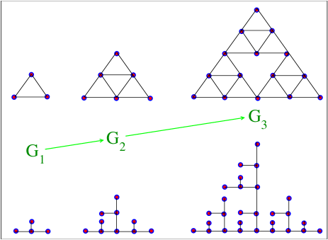
Figure 1: (Color online.) Recursive construction of the SG and of the TF.

For the SG one starts with three spins located on the vertexes of a triangle. This is the first generation $G_{1}$ of the structure. The second generation $G_{2}$ is obtained by considering three adjacent $G_{1}$ structures, building a larger triangular object. The process is then iterated at will. A similar construction is used for the TF, as shown in Fig. 1, the first generation is $G_{1}$ and the generation $G_{n}$ can be built attaching 3 $G_{n-1}$ structures in a single site. We will denote with $R_{n}$ the size of the finite generation $G_{n}$ i.e. the maximum distance between two sites of $G_{n}$. The fractal and spectral dimensions of the TF and of the SG can be analytically evaluated by means of exact renormalizations rammal , yielding $d_{f}=\log(3)/\log(2)$, $d_{s}=\log(9)/\log(6)$ and $d_{f}=\log(3)/\log(2)$, $d_{s}=\log(9)/\log(5)$ respectively. We consider the graphs obtained from the product of two SG’s (SGxSG) and two TF’s (TFxTF), their fractal and spectral dimensions can be calculated from Equations (4) obtaining $d_{f}=3.17..$, $d_{s}=2.45...$ for the TFxTF and $d_{f}=3.17..$, $d_{s}=2.73...$ for the SGxSG. Since $d_{s}>2$ the Ising model present a phase transition at finite temperature $T_{c}$, according to the generalized Froelich-Simon-Spencer bound fssgen .

III Models and Scaling Relation

In this section we introduce the model, the dynamical quantities of interest and overview their known scaling behavior. We consider, on a given graph ${\cal G}$, the Ising model, defined by the Hamiltonian

$$H[\sigma]=-J\sum_{<ij>}\sigma_{i}\sigma_{j}\equiv-J\sum_{i,j}A_{i,j}\sigma_{i}\sigma_{j}$$ (5)

where $\sigma_{i}=\pm 1$ denotes the spin of site $i$, $<ij>$ are nearest neighbors on the graph and $A_{i,j}$ is the adjacency matrix. The dynamics is introduced by randomly choosing a single spin and updating it with Metropolis transition rates:

$$w([\sigma]\to[\sigma^{\prime}])=\min\left[1,\exp(-\Delta E/(K_{B}T))\right].$$ (6)

Here $[\sigma]$ and $[\sigma^{\prime}]$ are the spin configurations before and after the move, $K_{B}$ is the Boltzmann constant, and

$$\Delta E=H[\sigma^{\prime}]-H[\sigma].$$ (7)

A Montecarlo time step is a sequence of $N$ random moves where $N$ is the number of sites in the finite realization of the graph $\cal{G}$. We will focus on the non-equilibrium situation where a completely random initial configuration, corresponding to an equilibrium state at $T=\infty$, is instantaneously quenched to a temperature equal or smaller than $T_{c}$.

III.1 Quenches to $T_{c}$

After quenching our system to the critical temperature, the two-time correlation function in the case of Ising variables is defined as

$$C_{ij}(t,s)=\langle\sigma_{i}(t)\sigma_{j}(s)\rangle$$ (8)

($\langle\ldots\rangle$ being an average over initial conditions and thermal histories). On a homogeneous structure (i.e. a lattice) for sufficiently large times (8) takes the scaling form godluck ; cal

$$C_{ij}(t,s)=L(s)^{-bz}g\left[\frac{r}{L(s)},\frac{L(t)}{L(s)}\right]$$ (9)

where $L(t)\propto t^{1/z}$ is the typical length associated to the growth of the critical phase, $z$ is the usual equilibrium dynamic exponent relating the relaxation time to the coherence length $\tau\propto\xi^{z}$, $r$ is the Euclidean distance between sites $i$ and $j$, $g(x,y)$ is a scaling function, and $bz=d-2+\eta$ is an exponent related to the usual equilibrium critical one $\eta$. The scaling form (9) is determined by the growth of correlated regions of size $L(t)$ with a fractal dimension $D_{f}=d-zb/2$ coniglio . Notice that when $d\to d_{L}$, $T_{c}\to 0$ and $b\to 0$. Then $D_{f}\to d$ and these regions grow compact. For instance, for the Ising model we are considering here one has $\eta=1$ at $d=d_{L}=1$, leading to $b=0$. This is a manifestation of the fact that the quench at $d_{L}$ is not a critical quench, but rather resembles a quench in the ordered phase, as it will be discussed in Sec. III.2. Let us remark that the analysis of the out of equilibrium process provides the equilibrium static and dynamic exponents, since they enter the form (9).

In the case of inhomogeneous structures, one might still expect some sort of scaling to hold. However, in that case a unique definition of distance $r$ is not available. Hence, in what follows, it will be useful to introduce the space integrated correlation function

$$F_{G}(t)=\sum_{i,j\in{G}}C_{ij}(t,t),$$ (10)

where $G$ is a certain subset of sites, which has the advantage of a straightforward generalization to fractal structures. Notice that we have restricted the definition to the equal time correlation $s=t$, since only this function will be considered in Sec. IV. In the case of homogeneous lattices, considering a box $G$ of size $R$, using Eq. (9) and $L(t)\propto t^{1/z}$, one finds

$$F_{G}(t)=t^{-b+d/z}f\left[\frac{R}{t^{1/z}}\right].$$ (11)

On an inhomogeneous structure such as the TFxTF or the SGxSG we will consider the quantity

$$F_{G_{k}}(t)=\sum_{i,j\in{G_{k}}}C_{ij}(t,t),$$ (12)

where sites are summed over the internal sites of the $k$-th generation $G_{k}$, for which we expect the scaling

$$F_{G_{k}}(t)=t^{-b+d_{f}/z}f\left[\frac{R_{k}}{t^{1/z}}\right].$$ (13)

On fractals the scaling hypothesis is hence naturally defined by Eq. (13) where the scaling function $f$ depends on ${R_{k}}/{t^{1/z}}$ only. Notice that the use of Eq. (13) avoids the problem of the definition of a distance, since the length $R_{k}$ is naturally associated to the $k$-th generation.

In Sec. (IV) we will study in detail the so called autocorrelation function, obtained by letting $i=j$ in Eq. (8). We do this not only because it is very often considered in aging systems, but also because, being an on-site quantity, it circumvents the definition of distances. In homogeneous systems this quantity does not depend on position and, denoting it as $C(t,s)$, from Eq. (9) and $L(t)\propto t^{1/z}$ one has the scaling behavior

$$C(t,s)=s^{-b}h\left(\frac{t}{s}\right),$$ (14)

with $h(t/s)=g[0,L(t)/L(s)]$. In equilibrium conditions, $C(t,s)$ is associated to the autoresponse function $R(t,s)=\left.\delta\langle\sigma_{i}\rangle/\delta h_{i}(s)\right|_{h_{i}=0}$, describing the effect of an impulsive perturbing magnetic field $h_{i}(s)$ switched on at time $s$ on site $i$, by the fluctuation-dissipation theorem $TR(t,s)=-dC(t,s)/ds$. When the system is out of equilibrium after a quench to $T_{c}$, the fluctuation-dissipation theorem no longer holds in general. However, in the short time difference regime, $t/s\simeq 1$, due to local equilibrium, observables such as $C$ and $R$ behave as in equilibrium noiteff ; noiegamba . The constraint imposed by the fluctuation-dissipation theorem, then, determines the value $a=b$ of the exponent entering the scaling form godluck ; cal ; noiteff ; noiegamba of $R$

$$R(t,s)=s^{-(a+1)}\hat{h}\left(\frac{t}{s}\right).$$ (15)

With the scalings (14,15) and $a=b$, the fluctuation-dissipation ratio

$$X\left(\frac{t}{s}\right)=T\frac{R(t,s)}{\frac{\partial C(t,s)}{\partial s}}$$ (16)

is a function of $t/s$. Its limiting value

$$X_{\infty}=\lim_{s\to\infty}\lim_{t\to\infty}X\left(\frac{t}{s}\right)$$ (17)

is of a particular interest, since it was shown godluck ; cal to be an universal quantity. For the Ising model in $d=2$ one has $X_{\infty}\simeq 0.33$ prendidacorbandolo . On inhomogeneous structures, since the autocorrelation function and the autoresponse may be site dependent, we define them as $C(t,s)=(1/N)\sum_{i}C_{ii}(t,s)$ and similarly for $R(t,s)$, where $N$ is the number of sites of the finite realization of the infinite graph $\cal{G}$.

III.2 Quenches below $T_{c}$

When the quench is performed below $T_{c}$ the nature of the process changes, because the target equilibrium state is ordered (magnetized) and degenerate. In this case domains of the two possible equilibrium phases grow, and their geometry is compact. The observable quantities introduced above split into two contributions bouchaudealtrienoi

$$C(t,s)=C_{st}(t-s)+C_{ag}(t,s),$$ (18)

and similarly for the other ones. The first stationary term is a quasi-equilibrium contribution provided by the interior of the domains, which is in fact equilibrated in one of the two possible phases. What is left over, the non-equilibrium character due to presence of the interfaces, contributes with the second term, which takes the scaling form (14) with $b=0$ (due to the compact geometry of the domains and the above-mentioned relation between $b$ and $D_{f}$). Similarly, for the aging part of the response function one has scaling as in Eq. (15). At variance with critical quenches, there is no known relation between the exponent $a$ and $b$, nor with any other equilibrium or non-equilibrium exponent. In two dimensions the value $a=1/4$ has been conjectured, and numerical simulations tend to conform to this hypotheses noi (although the value $a=1/2$ has been also reported henkel ). It is also known that $a>0$ for $d>d_{L}$, and that $a\to 0$ when $d\to d_{L}$. Hence, the value of the exponents $a$ and $b$, when $d$ is lowered towards $d_{L}$ approach the value $a=b=0$ both along the path of critical quenches (at $T=T_{c}$) or along the route with $T=0$ (or any route with $T<T_{c}$). However, as explained in noiteff the quench at $d=d_{L},T=0$ cannot be regarded as critical, but rather as a quench in the ordered phase, as it is clear since the equilibrium state at $T=0$ is degenerate and magnetized. Finally, let us recall that $a>0$ and $b=0$ implies that $X_{\infty}=0$ through Eqs.(16,17).

III.3 What is known about $a$ and $X_{\infty}$ on inhomogeneous structures

We have already discussed the fact that on Euclidean geometries one always finds $a>0$ in the phase-ordering kinetics of systems above $d_{L}$, while $a=0$ at $d_{L}$ noiteff ; lipzan . Elaborating on this, in nostriscalari ; noivec it was conjectured that a similar property holds also on inhomogeneous structures, and the exponent $a$ was proposed to infer the presence/absence of a finite temperature transition on a graph. Indeed $a=0$ was found on structures such as the SG, the TF and others where a magnetized state cannot be sustained at any finite temperature, whereas $a>0$ was observed for instance on the toblerone lattice (the product graph between the SG and the line) where $T_{c}>0$. Regarding the limiting fluctuation-dissipation ratio, the data reported in nostriscalari yield results very well compatible with the value $X_{\infty}=1/2$ observed in the $d=1$ homogeneous case nota , on all the structures with $a=0$ considered. Apart from $a$ and $X_{\infty}$, other exponents such as $z$ were found to be temperature dependent. In conclusion, all the graphs with $T_{c}=0$ considered in nostriscalari share the same value for two universal quantities, $a$ and $X_{\infty}$, with the usual 1d lattice.

IV Numerical results: Quench at $T_{c}$

In the following we will study the critical behavior of the product graphs TFxTF and SGxSG. In the simulations we used finite fractals of generation 7 so that the total number of sites equals 4787344 for the TFxTF and 1199025 for the SGxSG. We verified that the graph size is large enough to avoid finite size effects so that average quantities such as $C(t,s)$ turn out to be independent of the size $N$. In the following we will set $K_{B}=1$ and $J=1$. We will consider first the scaling of the equal time correlation $F_{G_{k}}(t)$, which, as a byproduct, allows one to determine $T_{c}$, and then the properties of two-time quantities.

IV.1 Determination of $T_{c}$ and scaling of $F_{G_{k}}(t)$

In order to determine $T_{c}$ we have followed two methods. The first makes use of the critical finite-size scaling of $F_{G_{k}}(t)$, Eq. (13). This form holds right at $T_{c}$, with $b>0$. Instead, above $T_{c}$ there is a departure from scaling at large times, since the system eventually equilibrates. Below $T_{c}$, a similar scaling form holds but only for the aging part of the correlation (recalling the discussion around Eq. (18)), and with the value $b=0$ characteristic of phase-ordering. In conclusion one expects to observe deviations from the scaling (13) with $b>0$ as one moves away from $T_{c}$. Hence, the method we use for determining $T_{c}$ amounts to the computation of $F_{G_{k}}(t)$ at several temperatures, trying to collapse the data according to Eq. (13) by plotting $t^{b-d_{f}/z}F_{G_{k}}(t)$ against $R_{k}/t^{1/z}$, using $T$, $b>0$ and $z$ are fitting parameters. More precisely, using the least square method, we introduce a quantity $S(T,z,b)$ with the meaning of a variance around the optimal value (see the Appendix for a precise definition). $S(T,z,b)$ measures the quality of the collapse and then we determine $T_{c}$, $z$ and $b$ as the values that provide the minimum of $S(T,z,b)$. Examples of data collapsed in this way are shown in Fig. 2 for the TFxTF. In the three panels we show the behavior of the curves collapsed with the optimal choice of $T_{c}$, $z$, $b$ (upper panel) or with other choices of $T$ (larger and smaller than the optimal one, which turns out to be $T_{c}=3.21$) for which $S(T,z,b)$ is slightly larger than the minimum. It is clearly observed that the collapse is better in the first case.

The next point is to give an estimate of the errors. It must be stressed here that statistical errors are quite small in our simulations, whereas the major source of inaccuracy is a systematic effect due to having a finite window of times $t$ and of sizes $R_{k}$. Therefore, in order to estimate the errors on the fitting parameters $T_{c}$, $z$, $b$, we define a compatibility region, namely a region around the optimal value of the parameters where the value of $S(T,z,b)$ is not larger than $n$ times the minimum. Here $n$ is the tolerance that we fix to $n=3$ (this value was chosen arbitrarily, but we have checked that different choices, ranging from $n=2$ to $n=5$, do not change the compatibility region significatively). An example of this procedure is depicted in Fig. 3 (left panel). Here, since we have three parameters, for the purpose of visualization we have fixed one of them, the temperature, to its optimal value and we have plotted the projection of the compatibility regions (for the TFxTF and SGxSG) on the $z,b$ plane. The right panels show that the collapse of the curves for the SGxSG gets worst when one moves from the optimal value of the parameters, in the centre of the compatibility region, to the border. From the determination of the compatibility region we can eventually associate an error to the determination of $T_{c}$, $z$, $b$ as the distance between the optimal value and the border of the region. This whole procedure provides the following values $T_{c}=3.21\pm 0.02$, $b=0.4\pm 0.15$, $z=2.6\pm 0.6$ for the TFxTF, and $T_{c}=6.14\pm 0.02$, $b=0.3\pm 0.15$, $z=2.8\pm 0.6$ for the SGxSG. The errors on $z$ and $b$ are quite large, therefore within this approach it is not clear if the critical behavior is characterized by the same exponents for our different structures. However Fig. 3 evidences that it is very unlikely that both exponents are equal because the compatibility regions do not intersect.

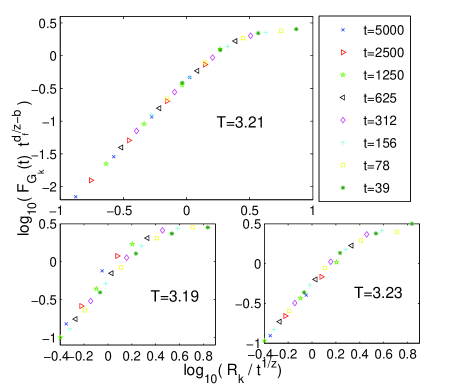
Figure 2: (Color online.) Data collapse obtained by plotting $t^{b-d_{f}/z}F_{G}(t)$ against $R_{k}/t^{1/z}$ for the TFxTF at three temperatures, $T=3.21\simeq T_{c}$ (upper panel), $T=3.19$ (lower left panel) and $T=3.23$ (lower right panel). Different points are evaluated on TFxTF of generation $k$ with $k$ ranging from 3 to 7. The value of $S(T,z,b)$ is $6\cdot 10^{-4}$ at $T=3.21$, $3\cdot 10^{-3}$ at $T=3.19$ and $2\cdot 10^{-3}$ at $T=3.23$

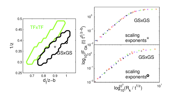
Figure 3: (Color online.) In the left panel, continuous lines enclose the parameter compatibility regions (see text) for the TFxTF and the SGxSG. The right panel represents the data collapse for $F_{G_{k}}(t)$ on the SGXSG. Upper plot is obtained by using as scaling exponents the value of the center of the compatibility region, evidencing a very good data collapse. The lower panel refers to values of the exponents at the border of the compatibility region. Notice that already for $n=3$ the scaling is sensitively worse, this evidence the reliability of the definition of the compatibility region.

Comparing the values of $T_{c}$ for the TFxTF and the SGxSG with the values of the lattice in two, three and four dimensions (i.e. $T_{c}\simeq 2.27$, $T_{c}\simeq 4.51$ and $T_{c}\simeq 6.68$) one observes that $T_{c}$ tends to increase with the average coordination number of the graph. However, clearly other non-universal parameters play a relevant role in determining the critical temperature, as can be noticed from the fact that the SGxSG and the 4-dimensional lattice have both $z_{i}=8$ but a different value of $T_{c}$.

The second method for the determination of $T_{c}$ makes use of the scaling properties of $C(t,s)$, as proposed and discussed in sarralip . With this technique we obtained results in agreement with the first method. Let us stress the advantage of these non-equilibrium methods, since there is no need to equilibrate the system which, due to the critical slowing down, is a very demanding numerical task.

IV.2 Scaling of two-time quantities

Letting $T=T_{c}$, we have computed the two-time quantities $C(t,s)$ and $R(t,s)$. In view of Eq. (14), by plotting $C(t,s)$ for fixed values of $t/s$ against $s$, (left panel of Fig. 4 and Fig. 5) we have determined the value $b=0.33\pm 0.03$ for the TFxTF and $b=0.39\pm 0.03$ for the SGxSG, in good agreement with the previous determination obtained through $F_{G}(t)$. Notice that the two time approach provides a much more precise value of $b$: indeed a single scaling exponent have to be fitted while in the scaling approach to $F_{G_{k}}(t)$ both the exponents $b$ and $1/z$ are evaluated numerically. Reconsidering the results of Sec. IV.1, we obtain also a better estimate of the $z$’s, which turn out to be $z=2.9\pm 0.3$ and $z=2.4\pm 0.2$ for the TFxTF and SGxSG respectively. Notice that these values (particularly $b$) are very different from those known for the homogeneous 2d lattice, namely $b\simeq 0.115$ and $z\simeq 2.17$. With a good confidence one may also conclude that they are different also for the two product graphs (although, in principle, the values $b=0.36$, $z=2.2$, obtained at the upper/lower limit of the error bars could be compatible with both the structures). The data collapse obtained by plotting $s^{b}C(t,s)$ against $t/s$ can be checked in the right panel of Fig. 4 and 5. For large values of $t/s$ the collapse is very good. Deviations are observed in the small $t/s$-region, but these appear to become less important as $s$ increases. This is a quite common feature in phase-ordering, observed also on homogeneous lattices, and can be attributed to pre-asymptotic corrections noiegamba ; noi ; preas .

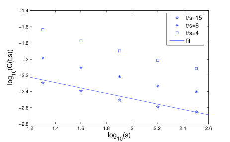
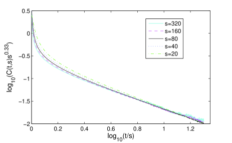
Figure 4: (Color online.) Left panel: Plot of $C(t,s)$ against $s$ for different fixed values of $t/s$ for the TFxTF quenched to $T_{c}$. The continuous line is the power law $s^{-b}$ with $b=0.33$. Right panel: Data collapse obtained by plotting $s^{b}C(t,s)$ against $t/s$, for several values of $s$.

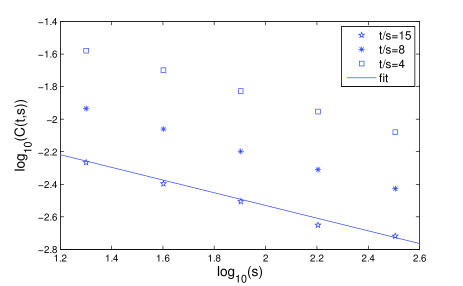
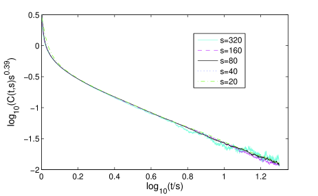
Figure 5: (Color online.) Left panel: Plot of $C(t,s)$ against $s$ for different fixed values of $t/s$ for the SGxSG quenched to $T_{c}$. The continuous line is the power law $s^{-b}$ with $b=0.39$. Right panel: Data collapse obtained by plotting $s^{b}C(t,s)$ against $t/s$, for several values of $s$.

For the computation of the response function we have used the field-free algorithm introduced in lippiello05 . We have checked that the scaling form (15) is obeyed with an exponent consistent with the expected behavior $a=b$. In Fig. 6, we plot the fluctuation-dissipation ratio against $s/t$, for different values of $s$. The good data collapse observed confirms that $R$ scales as in Eq. (15), with $a=b$. For $s/t\simeq 1$, in the quasi-equilibrium regime, there are no sensible deviations from the fluctuation-dissipation theorem, as discussed in Sec. III.1, and $X\simeq 1$. For $s/t\ll 1$ the so called aging regime is accessed, ad $X$ lowers. Extrapolating the intercept at $s/t=0$ we obtain $X_{\infty}=0.36\pm 0.03$ for the TFxTF and $X_{\infty}=0.40\pm 0.03$ for the SGxSG. Notice that these values are compatible within error bars. However, by comparing these values with the one ($X_{\infty}\simeq 0.33$) measured in the usual square lattice, one sees that for the TFxTF they are only marginally compatible, while for the SGxSG they are totally incompatible.

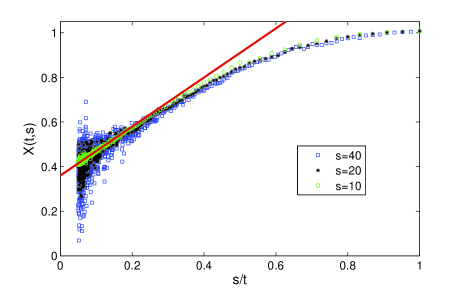
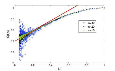
Figure 6: (Color online.) Plot of $X(t,s)$ against $s/t$ for different fixed values of $s$ for the TFxTF (left) and SGXSG (right) quenched to $T_{c}$.

In conclusion, in the case of critical quenches of the Ising model on the product structures considered here one finds a finite $T_{c}$ and a pattern of behaviors analogous to that found on homogeneous lattices. The value of the universal (on usual lattices) quantities $a$ and $X_{\infty}$, appear to be different between the TFxTF, the SGxSG and the 2d lattice.

V Numerical results: Quench below $T_{c}$

For completeness, for the TFxTF we have computed the value of the exponent $a$ also in the case of a quench below $T_{c}$ ($X_{\infty}$ is trivially zero in this process, see discussion at the end of Sec. III.2). It must be recalled that in the Toblerone lattice an exponent $a$ was found, whose value was compatible with the value $a=1/4$ found in the two-dimensional case. This could suggest that the conjecture discussed above, namely that products of 1d-like graphs could form a sort of universality class sharing the exponent $a$, although not confirmed by our previous data in critical quenches, could hold at least restricting to subcritical quenches. In order to check this issue we have computed the integrated response function $\chi(t,s)=\int_{s}^{t}dt^{\prime}R(t,t^{\prime})$ and, recalling the additive form discussed in Sec. III.2, we have isolated the aging term $\chi_{ag}$ by using a dynamics where flips of spin in the bulk are forbidden, as discussed in nostriscalari ; noi . From Eq. (15) one has

$$\chi_{ag}(t,s)=s^{-a}\tilde{h}(t/s),$$ (19)

where $\tilde{h}(x)$ is another scaling function. The data of Fig. (7) show that a good scaling collapse is obtained with an exponent $a=0.13\pm.02$ which is different from the value found in $d=2$ (see inset of Fig. (7) ). The fact that $a$ takes a comparable value in the $d=2$ homogeneous lattice and on the Toblerone lattice, therefore, seems not to be a general property of product graphs.

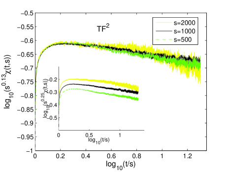
Figure 7: (Color online.) $s^{a}\chi{}(t,s)$, with $a=0.13$, is plotted against $t/s$ for different fixed values of $s$ for the TFxTF quenched to $T=3.0<T_{c}$. In the inset we plot $s^{0.25}\chi{}(t,s)$ against $t/s$ showing that for $a=1/4$ the scaling is not satisfied.

VI Discussion and conclusions

In this paper we have studied the scaling properties of the Ising model quenched to or below the critical temperature on graphs obtained by making direct products of 1d-like structures, such as the TFxTF and the SGxSG. The direct product is a convenient tool to build graphs with a topology sustaining a finite $T_{c}$, where the critical properties can be studied. This allows one to investigate the critical properties of such structures and to determine the critical exponents. Moreover, dynamical aspects can also be considered, by studying the evolution after temperature quenches. The aim of our analysis is to check the validity of dynamical scaling on inhomogeneous structures, and to study the behavior of the (limiting) fluctuation-dissipation ratios and of the scaling exponents. On regular lattices these are well understood and their universal properties are well known. On product graphs we found a non-equilibrium scaling behavior similar to that found on homogeneous lattices above $d_{L}$, where time enters observable quantities through a single growing length representing the size of the critical correlations established. Regarding the quantities which on homogeneous lattices are universal, previous studies of phase-ordering on a certain class of graphs showed their dependence on several parameters, among which the temperature, at variance with the regularity observed on homogeneous lattices. A notable exception was represented by the exponent $a$ and the limiting fluctuation-dissipation ratio $X_{\infty}$, which were found to take the same values $a=0$ and $X_{\infty}=1/2$ on all the graphs with $T_{c}=0$ considered insofar. In this paper we have considered the possibility that such a regularity could be extended to the various direct products of these $T_{c}=0$ graphs than one can consider, by studying if critical exponents or $X_{\infty}$ take a unique value for all the graphs of this class. The results we found, however, are negative in this respect, either in critical quenches or in sub-critical quenches. Indeed we have shown that product graphs exhibit different exponents, including $a$, and, restricting to critical quenches, also a different value of $X_{\infty}$. This may indicate that a robust universality property as observed on usual lattices is lost in the realm of inhomogeneous structure, or that, if some analogue of it exists, the relevant parameters of the graph topology determining universality have not yet been identified.

Appendix

We define the quality of the collapse between the different curves as follows. First, for every time $t_{i}$ we fit the curve $\log(F_{G_{k}}(t_{i}))$ as a function of the size $R_{k}$ with a polynomial of the form $\tilde{F}(t_{i},x)$ where $x=\log(R_{k}/t_{i}^{1/z})$. This is done since the function $F_{G_{k}}(t)$ is known only on a discrete set of sizes $R_{k}$. The curves $\hat{F}(x,t_{i})=\log(t_{i}^{b-d_{f}/z})+\tilde{F}(t_{i},x)$, obtained at different times $t_{i}$ should collapse once plotted against $x$ (the reason for taking the logarithms is that, since one has power-law dependences, the logarithms allow one to better take into account deviations from perfect collapse on a wide range of sizes and times). Then we introduce a squared distance between the rescaled curves as

$$S\left(T,z,b\right)=\sum_{i}\int\left[\hat{F}(x,t_{i})-\hat{F}(x,t_{i+1})\right]^{2}dx$$ (20)

References

- (1) T. Nakayama, K. Yakubo and R.L Orbach, Rev. Mod. Phys. 66, 381 (1994).
- (2) D.A.Beysens, G. Forgacs, J.A. Glazier, Proc. Nat. Ac. Sci. 97, 9467 (2000); C. Castellano. M. Marsili, A. Vespignani, Phys. Rev. Lett. 85, 3536 (2000).
- (3) D. Cassi, Phys. Rev. Lett. 76, 2941 (1996); R. Burioni , D. Cassi, and C. Destri, Phys. Rev. Lett. 85, 1496 (2000).
- (4) R. Burioni, D. Cassi, and A. Vezzani, Phys. Rev. E 60, 1500 (1999);
- (5) S. Alexander, and R. Orbach, J. Phys. Lett. 43, L62 (1982); K. Hattori, T. Hattori, and H. Watanabe, Prog. Theor. Phys. Suppl. 92, 108 (1987).
- (6) D. Cassi, L. Fabbian, J. Phys. A 32, L93 (1999).
- (7) R.Campari and D. Cassi, Phys. Rev. E 81, 021108 (2010); A. Vezzani, J. Phys. A 37, 37 (2004).
- (8) R. Burioni, D. Cassi, F. Corberi, and A. Vezzani, Phys. Rev. Lett. 96, 235701 (2006); Phys. Rev. E 75, 011113 (2007).
- (9) F. Harary, Graph theory, (Addison–Wesley, Reading, MA 1969); R. Cohen and S. Havlin, Complex Networks Structure, Robustness and Function (Cambridge University Press 2010)
- (10) B.Mohar and W. Woess Bull. London Math. Soc. 21, 209 (1989).
- (11) R.Burioni, D.Cassi and A. Vezzani, Eur. Phys. J. B 15 665 (2000); R.Burioni, D.Cassi, J. Phys. A 38 R45 (2005).
- (12) Y.Gefen, A.Aharony and B.B.Mandelbrot, J. Phys. A 16 1267 (1983); Y.Gefen, A.Aharony, Y. Shapir and B.B.Mandelbrot, J. Phys. A 17 435 (1984).
- (13) R.Rammal J. Physique 45 191 (1984).
- (14) C. Godréche, and J.M.Luck, J. Phys.:Cond. Matt. 14, 1589 (2002);
- (15) P. Calabrese and A. Gambassi A, J.Phys. A 38, R133 (2005).
- (16) A. Coniglio, Physica A 281, 129 (2000)
- (17) F. Corberi, E. Lippiello, M. Zannetti, J. Stat. Mech.: Theory and Experiment, P12007 (2004).
- (18) F. Corberi, A. Gambassi, E. Lippiello, and M. Zannetti, J. Stat. Mech.: Theory and Experiment, P02013 (2008).
- (19) P. Mayer, L. Berthier, J. P. Garrahan, and P. Sollich, Phys. Rev. E 68, 016116 (2003); C. Chatelain, J . Phys. A 36, 10739 (2003); F. Sastre, I. Dornic, and H. Chaté, Phys. Rev. Lett. 91, 267205 (2003); C. Chatelain, J. Stat. Mech.: Theory and Experiment, P06006 (2006).
- (20) J.P. Bouchaud, L.F. Cugliandolo, J. Kurchan, and M. Mézard, Out of equilibrium dynamics in spin glasses and other glassy systems, in Spin Glasses and Random Fields edited by A.P.Young (World Scientific, Singapore, 1997); A. Crisanti, and F. Ritort , J.Phys.A: Math.Gen. 36, R181 (2003).
- (21) F. Corberi, E. Lippiello, and M. Zannetti, Phys.Rev. E 63 06150629 (2001); Eur.Phys.J.B 24 359 (2001); Phys.Rev.Lett. 90 099601 (2003); Phys.Rev. E 68 046131 (2003); Phys. Rev. E 72, 028103 (2005); Phys. Rev. E 74, 041113 (2006).
- (22) M. Henkel, M. Pleimling, C. Godreche, and J.M. Luck, Phys. Rev. Lett. 87, 265701 (2001); M. Henkel, M. Paessens, and M. Pleimling, Phys.Rev. E 69, 056109 (2004).
- (23) E. Lippiello, and M. Zannetti, Phys.Rev. E 61, 3369 (2000); C. Godréche, and J.M. Luck, J.Phys.A: Math.Gen. 33, 1151 (2000).
- (24) R. Burioni, F. Corberi, and A. Vezzani, J. Stat. Mech.: Theory and Experiment, P02040 (2009).
- (25) This property was not shown in nostriscalari .
- (26) E. Lippiello, and A. Sarracino, arXiv:1003.4887.
- (27) F. Corberi, E. Lippiello and M. Zannetti, Phys. Rev. E 72, 056103 (2005); Phys.Rev. E 68, 046131 (2003)
- (28) E. Lippiello, F. Corberi, and M. Zannetti, Phys. Rev. E 71, 036104 (2005).