The criticality of self-assembled rigid rods on triangular lattices

Abstract

The criticality of self-assembled rigid rods on triangular lattices is investigated using Monte Carlo simulation. We find a continuous transition between an ordered phase, where the rods are oriented along one of the three (equivalent) lattice directions, and a disordered one. We conclude that equilibrium polydispersity of the rod lengths does not affect the critical behavior, as we found that the criticality is the same as that of monodisperse rods on the same lattice, in contrast with the results of recently published work on similar models.

Recently experimentalists have acquired the ability to control the interactions between colloidal particles, with dimensions in the nanometer-to-micrometer range, providing new windows into the structural and thermodynamic behavior of colloidal suspensions. Of particular interest are the so-called ”patchy colloids”, the surfaces of which are patterned so that they attract each other via discrete bonding sites (patches) of tunable number, size and strength. Some of the collective properties of patchy colloids are being intensively studied with theory and simulations of primitive models and a number of results have been obtained SciortinoReview2010 .

In systems with two bonding sites per particle, only (polydisperse) linear chains form and there is no liquid-vapor phase transition SciortinoChains2007 . If the linear chains are sufficiently stiff, however, they may undergo an ordering transition, at fixed concentration, as the temperature decreases below the bonding temperature. The description of self-assembled rods has to consider not only the effects of equilibrium polydispersity but also the polymerization process. In this context, we proposed a model of self-assembled rigid rods (SARR), composed of monomers with two bonding sites that polymerize reversibly into polydisperse chains Tavares2009a and carried out extensive Monte Carlo (MC) simulations to investigate the nature of the ordering transition of the model on the square lattice Almarza2010 . The polydisperse rods undergo a continuous ordering transition that was found to be in the 2D Potts q=2 (Ising) universality class, as in similar models where the rods are monodisperse Matoz2008b . This finding refutes the claim that equilibrium polydispersity changes the nature of the ordering transition of rigid rods on the square lattice from Ising to the Potts q=1 (percolation) universality class and questions a more recent one for a similar model on triangular lattices RamirezPastor2009 ; RamirezPastor2010a .

In this note we (re)examine the original model of SARR Tavares2009a ; Almarza2010 on triangular lattices (TL) using MC simulations. In the model a site is either empty or occupied by one monomer. Each monomer has two interacting patches pointing in opposite directions, $\pm{\bf s}$. The orientation (state) of the monomers, defined by the direction of the bonding patches, is restricted to the (three) lattice directions. The interaction potential can be described as follows: Provided that two particles, $i$ and $j$, occupy nearest-neighbor (NN) sites and provided that they are in the same state, the energy is lowered by an amount $\epsilon$ only if their orientations are fully aligned with the lattice vector ${\bf r}_{ij}$ (See Fig. 1). The bonding energy favors the self-assembly of rod-like lattice polymers (straight chains).

The Grand canonical Hamiltonian of the system is given by:

$$H=-\epsilon\sum_{i=1}^{M}\sum_{k=1}^{p}f(|{\bf s}({\bf r}_{i})\cdot{\hat{\alpha}}_{k}|)f(|{\bf s}({\bf r}_{i}+{\hat{\alpha}}_{k})\cdot{\hat{\alpha}}_{k}|)-\mu\sum_{i=1}^{M}|{\bf s}({\bf r}_{i})|,$$ (1)

where $i$ labels a lattice site, ${\hat{\alpha}}_{k};k=1,\cdots,p$, are unit vectors along the $p$ lattice directions ($p=3$ for TL); ${\bf s}({\bf r}_{i})$ denotes the orientation at a given lattice site: ${\bf s}({\bf r}_{i})={\bf 0}$ for an empty site, while for occupied sites ${\bf s}({\bf r}_{i})$ is equal to one of ${\hat{\alpha}}_{k}$ vectors; $M$ is the total number of sites; $f(x)=1$ if $x=1$, and zero otherwise; and $\mu$ is the chemical potential.

An ordering transition will occur as the average rod length increases. In the ordered phase the rods will align preferentially along one of the $p$ lattice directions (See Fig. 1). In this model, the only attractions between pairs of NN monomers are bonding ones. Additional lateral interactions that promote the condensation of monomers, leading to a competition between ordering of SARR and monomer condensation, are not considered, in line with the original SARR model Tavares2009a on the square lattice Almarza2010 ; RamirezPastor2009 . The presence of only two bonding patches and the absence of lateral interactions strongly suggest that the present model does not exhibit a discontinuous liquid-vapor transition at low temperatures SciortinoReview2010 ; SciortinoChains2007 ; Rouault .

Figure 1: Examples of ordered (left) and disordered (right) configurations for the SARR model on triangular lattices. Monomers are represented with thick segments lying on the lattice sites. Two nearest-neighbor monomers interact (and form a bond) if the corresponding segments are in a head-to-tail configuration.

The investigation of the ordering transition of SARRs on the TL is carried out through the analysis of the order parameter RamirezPastor2010a ,

$$\delta=\frac{|\sum_{k=1}^{3}N_{k}{\hat{\alpha}}_{k}|}{\sum_{k=1}^{3}N_{k}},$$ (2)

where $N_{k}$ is the number of monomers with orientation ${\hat{\alpha}}_{k}$.

In the Grand Canonical Ensemble, at a fixed chemical potential, the critical temperature, $T_{c}=T_{c}(\mu)$ is found by extrapolating to the thermodynamic limit the finite-size pseudo critical temperatures, $T_{c}(L)$, which may be defined in various ways ($L$ being the length of the rhombic simulation box; $M=L^{2}$). Given the symmetry of the model, one can use the fourth-order cumulant of the order parameter distribution Landau_Binder ; Weber , $g_{4}=<\delta^{4}>/<\delta^{2}>^{2}$, to define $T_{c}(L)$ as the temperature where the finite-size cumulant $g_{4}(T)$ takes the universal value, $g_{4c}$, for a given universality class and boundary conditions Landau_Binder . We assume that the criticality of polydisperse rods on the TL is the same as that of monodisperse rods on the same lattice, i.e., Potts $q=3$ Vink ; Matoz2008a . We emphasize that this assumption is made for (computational) convenience and does not constrain the determination of the critical behavior, as discussed below.

Although the value of $g_{4c}$ for the Potts q=2 model on the square lattice is well known Salas ; Kamienarz we have not found in the literature reliable estimates of $g_{4c}$ for the Potts $q=3$ model on TL with periodic boundary conditions, rhombic boxes, and order parameters defined as in Eq.(2). We have therefore estimated its value by running simulations of the Potts $q=3$ model at the critical temperatureWu , with the same box shape and boundary conditions, using the Swendsen-Wang algorithm Swendsen . Different system sizes in the range $12\leq L\leq 96$ were considered. The results were fitted to the scaling equation Bloete ,

$$g_{4}(L,T_{c})=g_{4c}+aL^{y_{i}},$$ (3)

where $g_{4c}$, $a$, and $y_{i}$ are obtained from fits of the simulation results or, alternatively, $y_{i}$ (the critical exponent associated to the so-called irrelevant field) is set to the theoretical value $y_{i}=-4/5$ Nienhuis ; Shchur . In the first case we find $y_{i}=-0.74\pm 0.10$ and $g_{4c}=1.168\pm 0.002$; while setting $y_{i}=-4/5$ leads to $g_{4c}=1.167\pm 0.001$. We have used the latter values in the finite-size scaling analysis reported below.

We carried out coupled Grand Canonical Ensemble MC simulations. For a fixed value of $\mu$ several values of the temperature, $T_{i}=T_{0}+i\Delta T$ (with $i=0,1,\cdots,N_{T}-1$), are sampled in a single MC run using a simulation tempering algorithm Zhang2007 . This is achieved using a probability function given by:

$$P({\bf S}^{M},T_{i})=\Omega(T_{i})\exp\left[-H({\bf S}^{M})/k_{B}T_{i}\right].$$ (4)

In order to obtain good sampling over all temperatures one has to use an appropriate weight function $\Omega(T_{i})$. This was computed through an equilibration procedure following the usual strategies of the Wang-Landau-type algorithmsZhang2007 ; Wang ; Lomba . This simulation tempering algorithm is known to enhance the sampling efficiencyZhang2008 .

After preliminary runs to locate the critical region we run long simulations using typically between $N_{T}=20$ and $N_{T}=40$ values of $T_{i}$ around the critical temperature. At each $\mu$ we considered different system sizes. As the interactions are restricted to NN, the lattices are split into three sublattices, where the sites do not interact energetically. Simulation runs are organized in sweeps. In a sweep we update the state of every site and attempt one temperature change. This is done by considering sequentially the three sublattices; we select for each site a new state ($k=0,1,2,3$) (with $k=0$ denoting an empty site) with probabilities depending on the interaction energy, the value of $\mu$ and of the current temperature. After updating all sites we attempt a temperature change by choosing at random (with equal probabilities) increasing or decreasing the current temperature by an amount $\Delta T$, and accept or reject the change by considering the probability given by Eq. (4), and the usual Metropolis criterion Landau_Binder . The length of a simulation run was $2\times 10^{8}$ sweeps, and the results were split into twenty blocks of $10^{7}$ sweeps for subsequent error analysis. In Figure 2 we illustrate the results for the order parameter close to the transition temperature, at two values of the chemical potential.

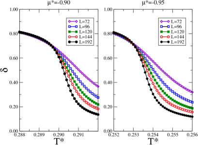
Figure 2: Results for the order parameter $\delta$ as a function of the reduced temperature for different system sizes (as indicated in the legends); left panel $\mu/\epsilon=-0.90$, right panel $\mu/\epsilon=-0.95$.

System-size dependent pseudo-critical temperatures, $T_{cL}=T_{c}(L)$ are computed by the matching criterion Wilding ,

$$g_{4}(L,T_{cL},\mu)=g_{4c},$$ (5)

where for convenience we set $g_{4c}$ to the universal value of the Potts $q=3$ universality class. Critical temperatures, $T_{c}$, were extrapolated by fitting the values $T_{c}(L)$ to scaling equations of the form,

$$T_{c}(L)=T_{c}+aL^{-b}.$$ (6)

In order to avoid biasing the analysis we used two values for the exponent $b$: $b=(1+\theta)/\nu$ Wilding ; Bloete with $\theta=-y_{i}\nu$ and $\nu=5/6$ Wu for Potts $q=3$ scaling, and $b=(1/\nu)_{q=1}=0.75$ for Potts $q=1$ Wu ; $\nu$ and $\theta$ are respectively the correlation length and Wegner’s correction to scaling exponents. However, the two values of $T_{c}$ were found to be very close. The critical temperatures $T_{c}$ collected in Table 1 are those computed using the Potts $q=3$ scaling, which are consistent with the temperatures where the Binder cumulants cross (see Figure 3). Notice that the crossing of the $g_{4}(T)$ curves for different values of $L$ deviates slightly from the computed value of $g_{4c}$. In order to constrain as little as possible the analysis of the criticality of SARRs on the TL we have computed secondary error bars (shown between curly brackets in Table 1) that include the estimates for the critical temperature found using the Potts $q=1$ scaling.

System	$\mu/\epsilon=-0.95$	$\mu/\epsilon=-0.90$	$\mu\rightarrow\infty$($\rho=1$)
n	11	13	9
$L_{min}$–$L_{max}$	84-192	72-192	60–144
$T_{c}^{*}$	0.25336(4){11}	0.29006(4){10}	0.47637(4){19}
$\rho_{c}^{*}$	0.597(3){9}	0.688(3){6}	–
$\beta/\nu$	0.110(22){57}	0.115(18){43}	0.126(9){31}
$\gamma/\nu$	1.69(7){19}	1.72(5){12}	1.70(4){12}
$1/\nu$	1.27(8){20}	1.28(6){12}	1.21(4){12}
$(\alpha/\nu)$	0.40(28){38}	0.43(25){33}	0.45(28){32}

Table 1: Finite-size scaling results from simulation: $n$ is the number of system sizes used to compute critical properties and effective critical exponents. $L_{min}$ and $L_{max}$ are the minimum and maximum system sizes used in the finite-size scaling analysis. The results shown for $\alpha/\nu$ were computed from the scaling of $(\partial\rho/\partial T)_{\mu}$, except for the full lattice case ($\rho=1$) where $(\partial(H/M)/\partial T)$ was used. For finite $\mu$ similar values of $\alpha/\nu$ were obtained using $(\partial\rho/\partial\mu)_{T}$ or $(\partial(H/M)/\partial T)_{\mu}$. The critical exponent ratios for Potts $q=1$ universality class are $\beta/\nu=5/48\simeq 0.104$, $\gamma/\nu=43/24\simeq 1.792$, $1/\nu=3/4$ and $\alpha/\nu=-1/2$. The corresponding values for Potts $q=3$ universality class are $\beta/\nu=2/15\simeq 0.133$, $\gamma/\nu=26/15\simeq 1.733$, $1/\nu=6/5$, and $\alpha/\nu=2/5$Wu . Error bars are given in parentheses (curly brackets) in units of the last digit of the corresponding quantity.

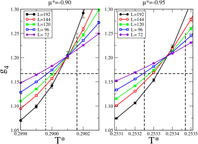
Figure 3: Fourth order Binder cumulant at constant $\mu$ as a function of $T$, for different system sizes; left panel $\mu/\epsilon=-0.90$, right panel $\mu/\epsilon=-0.95$. Horizontal lines depict the estimate of $g_{4c}$ for the two dimensional Potts q=3 universality class. Vertical lines delimit the unbiased estimates of the critical temperature (See the text for the details).

The critical behavior of the model was investigated by analyzing the system-size dependence of various properties at the extrapolated critical temperature. We fit the simulation results for a given property at $T_{c}$ to the expected scaling relation Landau_Binder $\delta(L)\propto L^{-\beta/\nu}$, $\chi(L)\propto L^{\gamma/\nu}$, and $(\partial\ln<\delta(L)>/\partial T)_{\mu}\propto L^{1/\nu}$, where $\chi(L)=L^{2}\left[<\delta^{2}>-<\delta>^{2}\right]/k_{B}T$. $\beta$ and $\gamma$ are the critical exponents for the order parameter and the susceptibility, respectively. In addition, the quantities proportional to the second derivatives of the Grand Potential per unit volume with respect to the temperature and/or chemical potential, $(\partial(H/M)/\partial T)_{\mu}$, $(\partial\rho/\partial T)_{\mu}$, and $(\partial\rho/\partial\mu)_{T}$, are fitted to non-linear equations of the form,

$$\left(\frac{\partial\rho}{\partial T}\right)_{\mu}=a_{0}+a_{1}L^{\alpha/\nu},$$ (7)

where $\rho$ is the density (fraction of occupied sites), and $\alpha$ is the specific heat critical exponent. In Fig. 4 we illustrate the $\rho$, and of its derivative $(\partial\rho/\partial T)_{\mu}$ at $\mu/\epsilon=-0.95$ around the critical temperature. In Table 1 we collect the estimates for the different critical exponents (or exponent ratios). The uncertainty in the estimate of $T_{c}$ was taken into account and as we did for the critical temperatures, two estimates of the error bars are given, with the second one corresponding to error bars that are sufficiently large to include the critical temperature found using the Potts $q=1$ scaling.

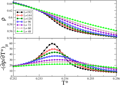
Figure 4: Density and derivative of the density with respect to the temperature at constant chemical potential $\mu/\epsilon=-0.95$.

For completeness we have computed the critical densities, by fitting the results to Wilding :

$$\rho_{c}(L,\mu,T_{cL})=\rho_{c}(\mu)+aL^{-2+1/\nu},$$ (8)

using the value of $\nu$ for the Potts $q=3$ universality class.

The results in table 1 clearly indicate that the critical behavior of the SARR model on the TL is much better described within the Potts $q=3$ than within the $q=1$ universality class. Given that the former critical behavior was observed in the monodisperse case, we conclude that equilibrium polydispersity does not affect the critical behavior of rigid rod models, in contrast with the conclusion of Lopez et al. RamirezPastor2010a . Even considering the largest error bars on the critical temperature, the values of the effective exponents $\nu$, and $\alpha/\nu$ are not compatible with Potts $q=1$ critical behavior. The deviations observed in the crossings of $g_{4}(T)$ for different system sizes from the estimated value of $g_{4c}$ is most likely due to the importance of scaling corrections (low absolute value of $y_{i}$).

In previously published work Almarza2010 we discussed the reasons for the apparent $q=1$ critical behavior observed by Lopez et al. on the square lattice RamirezPastor2009 . The apparent $q=1$ behavior observed by the same authors on the TL RamirezPastor2010a results also from using the density as the scaling variable. In fact, a simple but revealing analysis by FisherFisher , shows that fixing the density in models such as those discussed here, corresponds to introducing a constraint that renormalizes the critical exponents. For the Potts $q=3$ universality class the renormalized correlation length exponent $\nu_{X}$ is $\nu_{X}=\nu/(1-\alpha)=5/4$, which is close to the value of $\nu$ for the $q=1$ universality class $\nu_{q=1}=4/3$, reported by Lopez et al. RamirezPastor2010a .

- (1) F. Sciortino, Collect. Czech. Chem. Commun., 75, 349 (2010).
- (2) F. Sciortino, E. Bianchi, J. F. Douglas and P. Tartaglia, J. Chem. Phys. 126, 194903 (2007).
- (3) J. M. Tavares, B. Holder and M. M. Telo da Gama, Phys. Rev E 79, 021505 (2009).
- (4) N. G. Almarza, J. M. Tavares and M. M. Telo da Gama, Phys. Rev. E 82, 061117 (2010).
- (5) D. A. Matoz-Fernandez, D. H. Linares and A. J. Ramirez-Pastor, Europhys. Lett. 82, 50007 (2008).
- (6) L. G. López, D. H. Linares and A. J. Ramirez-Pastor, Phys. Rev E 80, 040105(R)(2009).
- (7) L. G. López, D. H. Linares and A. J. Ramirez-Pastor, J. Chem. Phys. 133 134702 (2010).
- (8) Y. Rouault and A. Milchev, Phys. Rev. E, 51, 5905 (1995).
- (9) D. P. Landau and K. Binder, ”A Guide to Monte Carlo Simulation in Statistical Physics, 2nd edition”, (Cambridge University Press 2005).
- (10) H. Weber, W. Paul, and K. Binder, Phys. Rev. E 59, 2168 (1999).
- (11) T. Fischer, and R. L. C. Vink, EPL, 85, 56002 (2009).
- (12) D. A. Matoz-Fernandez, D. H. Linares and A. J. Ramirez-Pastor, J. Chem. Phys. 128, 214902 (2008).
- (13) J. Salas and A. D. Sokal, J. Stat. Phys. 98, 551 (2000).
- (14) G. Kamienarz and H. W. J. Blöte, J. Phys. A: Math. Gen. 26, 201 (1993).
- (15) F. Y. Wu, Rev. Mod. Phys., 54, 235 (1982).
- (16) R. H. Swendsen and J.-S. Wang, Phys. Rev. Lett. 58, 86 (1987).
- (17) H. W. J. Blöte, E. Luijten, and J.R. Heringa, J. Phys. A: Math. Gen. 28, 6289 (1995).
- (18) B. Nienhuis, J. Phys. A: Math. Gen. 15, 199 (1982).
- (19) L. N. Shchur, B. Berche, and P. Butera, Phys. Rev. B 77, 144410 (2008).
- (20) C. Zhang and J. Ma, Phys. Rev. E, 76, 036708 (2007).
- (21) F. Wang and D. P. Landau, Phys. Rev. Lett. 86, 2050 (2001).
- (22) E. Lomba, N. G. Almarza, C. Martín and C. McBride, J. Chem. Phys. 126, 244510 (2007).
- (23) C. Zhang and J. Ma, J. Chem. Phys. 129, 134112 (2008).
- (24) N. B. Wilding, Phys. Rev. E 52, 602 (1995).
- (25) M. E. Fisher, Phys. Rev. 176, 257 (1968).