Optimal transport from Lebesgue to Poisson

Abstract

This paper is devoted to the study of couplings of the Lebesgue measure and the Poisson point process. We prove existence and uniqueness of an optimal coupling whenever the asymptotic mean transportation cost is finite. Moreover, we give precise conditions for the latter which demonstrate a sharp threshold at $d=2$. The cost will be defined in terms of an arbitrary increasing function of the distance.

The coupling will be realized by means of a transport map (“allocation map”) which assigns to each Poisson point a set (“cell”) of Lebesgue measure 1. In the case of quadratic costs, all these cells will be convex polytopes.

and

1 Introduction and statement of main results

(a) The theory of optimal transportation studies couplings between two probability measures $\lambda$ and $\nu$ on $\mathbb{R}^{d}$ which minimize the total transportation cost. A coupling is interpreted as a plan how to transport $\lambda$ into $\nu$. Transporting a unit of mass from $a$ to $b$ produces cost of amount $c(a,b)$, where $c(\cdot,\cdot)$ is a given cost function. Of particular interest are couplings $q$ which are induced by transport maps, that is, $q=(\mathrm{id},\psi)_{*}\lambda$ for some map $\psi\dvtx\mathbb{R}^{d}\to\mathbb{R}^{d}$ with $\psi_{*}\lambda=\nu.$

A fair allocation for a simple point process in $\mathbb{R}^{d}$ is a coupling of the Lebesgue measure $\mathfrak{L}$ and the point process $\mu^{\bullet}$ induced by a transport map, that is, there is a map $\Psi\dvtx\Omega\times\mathbb{R}^{d}\to\mathbb{R}^{d}$ such that for $\mathbb{P}$-almost every $\omega\in\Omega$ the map $\Psi^{\omega}\dvtx\mathbb{R}^{d}\to\mathbb{R}^{d}$ transports the Lebesgue measure into the point process: $\Psi^{\omega}_{*}\mathfrak{L}=\mu^{\omega}.$ Such an allocation is called factor allocation if it is a measurable function of the point process (i.e., it measurably depends only on the given point process).

In this article we connect these two theories by constructing fair allocations between the Lebesgue measure and point processes using tools from optimal transportation. Instead of considering the total transportation cost we ask for minimizers of the cost per unit mass. Good estimates on the transportation cost will directly imply good tail estimates for the distribution of the transport distance.

Moreover, the techniques developed in this article allow us to construct a fair factor allocation with the best possible tail estimate and also to derive new estimates on the transportation cost between the Lebesgue measure and a Poisson point process.

We now describe our results in more detail.

(b) A point process $\mu^{\bullet}\dvtx\Omega\to\mathcal{N}(\mathbb{R}^{d})$ is a random variable with values in the space of integer valued Radon measure. Put $\Xi(\omega)=\operatorname{supp}(\mu^{\omega}).$ Then, $\mu^{\bullet}$ has the representation $\mu^{\bullet}\dvtx\omega\mapsto\mu^{\omega}=\sum_{\xi\in\Xi(\omega)}k(\xi)\cdot\delta_{\xi}$ with $k(\xi)\in\mathbb{N}.$ $\mu^{\bullet}$ is called equivariant if for all Borel sets $A\in\mathcal{B}(\mathbb{R}^{d})$ we have $\mu^{\omega+z}(A+z)=\mu^{\omega}(A).$ Here, we interprete $\omega+z$ as the support of $\mu^{\omega}$ translated by $z$; see Section 2.2.

Given an equivariant point process $\mu^{\bullet}\dvtx\omega\mapsto\mu^{\omega}=\sum_{\xi\in\Xi(\omega)}k(\xi)\cdot\delta_{\xi}$ on $\mathbb{R}^{d}$ with unit intensity, we consider the set $\Pi$ of all couplings $q^{\bullet}$ of the Lebesgue measure $\mathfrak{L}$ and the point process—that is, the set of measure-valued random variables $\omega\mapsto q^{\omega}$ s.t. for a.e. $\omega$ the measure $q^{\omega}$ on $\mathbb{R}^{d}\times\mathbb{R}^{d}$ is a coupling of $\mathfrak{L}$ and $\mu^{\omega}$—and we ask for a minimizer of the asymptotic mean cost functional

$${\mathfrak{C}}_{\infty}\bigl{(}q^{\bullet}\bigr{)}:=\liminf_{n\to\infty}\frac{1}{\mathfrak{L}(B_{n})}\mathbb{E}\biggl{[}\int_{\mathbb{R}^{d}\times B_{n}}\vartheta\bigl{(}|x-y|\bigr{)}\,dq^{\bullet}(x,y)\biggr{]}.$$

Here $B_{n}:=[0,2^{n})^{d}\subset\mathbb{R}^{d}$. The scale $\vartheta\dvtx\mathbb{R}_{+}\to\mathbb{R}_{+}$ will always be some strictly increasing, continuous function with $\vartheta(0)=0$ and $\lim_{r\to\infty}\vartheta(r)=\infty.$

A coupling $\omega\mapsto q^{\omega}$ of the Lebesgue measure and the point process is called optimal if it minimizes the asymptotic mean cost functional and if it is equivariant in the sense that $q^{\omega+z}(A+z,B+z)=q^{\omega}(A,B)$ for all $z\in\mathbb{R}^{d}$ and Borel sets $A,B\in\mathcal{B}(\mathbb{R}^{d}).$ Our main result states the following:

Theorem 1.1

If the asymptotic mean transportation cost

$${\mathfrak{c}}_{\infty}:=\liminf_{n\to\infty}\inf_{q^{\bullet}\in\Pi}\frac{1}{\mathfrak{L}(B_{n})}\mathbb{E}\biggl{[}\int_{\mathbb{R}^{d}\times B_{n}}\vartheta\bigl{(}|x-y|\bigr{)}\,dq^{\bullet}(x,y)\biggr{]}$$ (1)

is finite, then there exists a unique optimal coupling of the Lebesgue measure and the point process $\mu^{\bullet}$.

(c) The unique optimal coupling $q^{\omega}$ can be represented as $(\mathrm{id},T^{\omega})_{*}\mathfrak{L}$ for some map $T^{\omega}\dvtx\mathbb{R}^{d}\to\mathrm{supp}(\mu^{\omega})\subset\mathbb{R}^{d}$ measurably only dependent on the sigma algebra generated by the point process. In other words, $T^{\omega}$ defines a fair factor allocation. Its inverse map assigns to each point $\xi$ of the point process (“center”) a set (“cell”) of Lebesgue measure $\mu^{\omega}(\xi)\in\mathbb{N}$. If the point process is simple, then all these cells have volume 1. In the case of quadratic cost, that is, $\vartheta(r)=r^{2}$, the cells will be convex polytopes. The transport map will be given as $T^{\omega}=\nabla\varphi^{\omega}$ for some convex function $\varphi^{\omega}\dvtx\mathbb{R}^{d}\to\mathbb{R}$ and induces a Laguerre tessellation; see lautensack2007 .

In the case $\vartheta(r)=r$ the transportation map induces a Johnson–Mehl diagram; see aurenhammer1991 . For the many results on and applications of these tessellations see the references in lautensack2007 and aurenhammer1991 . In the light of these results one might interpret the optimal coupling as a generalized tessellation.

(d) As a particular corollary to Theorem 1.1 we conclude that ${\mathfrak{c}}_{\infty}=\inf_{q^{\bullet}\in\Pi}{\mathfrak{C}}_{\infty}(q^{\bullet})$ and that the infimum is always attained; more precisely, it is attained by an equivariant coupling $q^{\bullet}$. For equivariant couplings $q^{\bullet}$ the mean cost functional $\frac{1}{\mathfrak{L}(A)}\mathbb{E}[\int_{\mathbb{R}^{d}\times A}\vartheta(|x-y|)\,dq^{\bullet}(x,y)]$, however, is independent of $A\subset\mathbb{R}^{d}$. Hence,

$${\mathfrak{c}}_{\infty}=\inf_{q^{\bullet}\in\Pi_{\mathrm{eqv}}}\mathbb{E}\biggl{[}\int_{\mathbb{R}^{d}\times[0,1)^{d}}\vartheta\bigl{(}|x-y|\bigr{)}\,dq^{\bullet}(x,y)\biggr{]},$$

where $\Pi_{\mathrm{eqv}}$ now denotes the set of all equivariant couplings of the Lebesgue measure and the point process.

Moreover, for equivariant couplings, $\mathbb{E}[\vartheta(|x-T^{\bullet}(x)|)]$ the mean cost of transportation of a Lebesgue point $x$ to the center of its cell is independent of $x\in\mathbb{R}^{d}$. Hence,

$$\mathfrak{c}_{\infty}=\inf_{T^{\bullet}}\mathbb{E}\bigl{[}\vartheta\bigl{(}\bigl{|}0-T^{\bullet}(0)\bigr{|}\bigr{)}\bigr{]},$$ (2)

where the infimum is taken over all equivariant maps $T\dvtx\mathbb{R}^{d}\times\Omega\to\mathbb{R}^{d}$ with ${T^{\omega}}_{*}\mathfrak{L}=\mu^{\omega}$ for a.e. $\omega$. And again: the infimum is attained by a unique such $T$. Let us point out that identity (2) allows us to resolve the asymmetry in the integration domain in equation (1): we equally well may replace the domain of integration $\mathbb{R}^{d}\times B_{n}$ by $B_{n}\times\mathbb{R}^{d}$.

(e) Analogous results will be obtained in the more general case of optimal “semicouplings” between the Lebesgue measure and point processes of “subunit” intensity.

We develop the theory of optimal semicouplings as a concept of independent interest. Optimal semicouplings are solutions of a twofold optimization problem: the optimal choice of a density $\rho\leq 1$ of the first marginal $\mu_{1}$ and subsequently the optimal choice of a coupling between $\rho\mu_{1}$ and $\mu_{2}$. This twofold optimization problem can also be interpreted as a transport problem with free boundary values; see Figure 1.

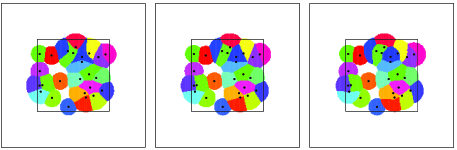
Figure 1: Optimal semicoupling of Lebesgue and 25 points in the cube with cost function $c(x,y)=|x-y|^{p}$ and (from left to right) $p=1,2,4$, respectively.

Given a point process of subunit intensity and finite mean transportation cost, we prove that there exists a unique optimal semicoupling between the Lebesgue measure and the point process. It can be represented on $\mathbb{R}^{d}\times\mathbb{R}^{d}$ as before as $q^{\omega}=(\mathrm{id},T^{\omega})_{*}\mathfrak{L}$ in terms of a transport map $T^{\omega}\dvtx\mathbb{R}^{d}\to\operatorname{supp}[\mu^{\omega}]\cup\{\eth\}$ where $\eth$ now denotes an isolated point (“cemetery”) added to $\mathbb{R}^{d}$.

(f) In any case, we prove that the unique transport map $T^{\omega}$ can be obtained as the limit of a suitable sequence of transport maps which solve the optimal transportation problem between the Lebesgue measure and the point process restricted to bounded sets.

More precisely, for $z\in\mathbb{Z}^{d}$ and $\gamma\in\Gamma:=(\{0,1\}^{d})^{\mathbb{N}}$ consider the “doubling sequence” of cubes

$$B_{n}(z,\gamma)=z-\sum_{k=1}^{n}2^{k-1}\gamma_{k}+\bigl{[}0,2^{n}\bigr{)}^{d}.$$

Note that the cube $B_{n}(z,\gamma)$ is one of the subcubes obtained by subdividing $B_{n+1}(z,\gamma)$ into $2^{d}$ cubes of half edge length. Let $T_{z,n}(\cdot,\omega,\gamma)\dvtx\mathbb{R}^{d}\to\operatorname{supp}[\mu^{\omega}]\cup\{\eth\}$ be the transport map for the unique optimal semicoupling between $\mathfrak{L}$ and $1_{B_{n}(z,\gamma)}\cdot\mu^{\omega}$, that is, for the optimal transport of an optimal “submeasure” $\rho^{\omega}\cdot\mathfrak{L}$ to the point process restricted to the cube $B_{n}(z,\gamma)$.

Theorem 1.2

For every $z\in Z^{d}$ and every bounded Borel set $M\subset\mathbb{R}^{d}$,

$$\lim_{n\to\infty}(\mathfrak{L}\otimes\mathbb{P}\otimes\nu)\bigl{(}\bigl{\{}(x,\omega,\gamma)\in M\times\Omega\times\Gamma\dvtx T_{z,n}(x,\omega,\gamma)\not=T(x,\omega)\bigr{\}}\bigr{)}=0,$$

where $\nu$ denotes the Bernoulli measure on $\Gamma$.

(g) If $\mu^{\bullet}$ is a Poisson point process with intensity $\beta\leq 1$ we have rather sharp estimates for the asymptotic mean transportation cost to be finite.

Theorem 1.3

(i) Assume $d\geq 3$ (and $\beta\leq 1$) or $\beta<1$ (and $d\geq 1$). Then there exists a constant $0<\kappa<\infty$ s.t.

$$\limsup_{r\to\infty}\frac{\log\vartheta(r)}{r^{d}}<\kappa\quad\Longrightarrow\quad{\mathfrak{c}}_{\infty}<\infty\quad\Longrightarrow\quad\liminf_{r\to\infty}\frac{\log\vartheta(r)}{r^{d}}\leq\kappa.$$

(ii) Assume $d\leq 2$ and $\beta=1$. Then for any concave $\hat{\vartheta}\dvtx[1,\infty)\to\mathbb{R}$ dominating $\vartheta$

$$\int_{1}^{\infty}\frac{\hat{\vartheta}(r)}{r^{1+d/2}}\,dr<\infty\quad\Longrightarrow\quad{\mathfrak{c}}_{\infty}<\infty\quad\Longrightarrow\quad\liminf_{r\to\infty}\frac{\vartheta(r)}{r^{d/2}}=0.$$

The first implication in assertion (ii) is new. Assertion (i) in the case $\beta=1$ is due to Holroyd and Peres extra-heads , based on a fundamental result of Talagrand Talagrand94 . The first implication in assertion (i) in the case $\beta<1$ was proven by Hoffman, Holroyd and Peres stable-marriage . The second implication in assertion (ii) is due to holroyd2001find .

Now let us consider the particular case of $L^{p}$ transportation cost, that is, $\vartheta(r)=r^{p}$.

Corollary 1.4

(i) For all $d\in\mathbb{N}$, all $\beta\leq 1$ and $p\in(0,\infty)$ the asymptotic mean $L^{p}$-transportation cost ${\mathfrak{c}}_{\infty}$ is finite if and only if

$$p<\overline{p}:=\cases{\infty,&\quad$\mbox{for }d\geq 3\mbox{ or }\beta<1;$\vspace*{2pt}\cr\displaystyle\frac{d}{2},&\quad$\mbox{for }d\leq 2\mbox{ and }\beta=1.$}$$

(ii) If $\beta=1$, then for all $p\in(0,\infty)$ there exist constants $0<k\leq k^{\prime}<\infty$ s.t. for all $d>2(p\wedge 1)$

$$k\cdot d^{p/2}\leq\mathfrak{c}_{\infty}\leq k^{\prime}\cdot d^{p/2}.$$

(h) The study of fair allocations for point processes is an important and hot topic of current research; see, for example, extra-heads , timar2008invariant , matching09 and references therein. A landmark contribution was the construction of the stable marriage between Lebesgue measure and an ergodic translation invariant simple point process stable-marriage . One of the challenges is to produce allocations with fast decay of the distance of a typical point in a cell to its center or of the diameter of the cell. The gravitational allocation gravity , phasegravity in $d\geq 3$ was the first allocation with exponential decay. Moreover, all the cells are connected and contain their center. However, the decay was not yet as good as the decay of a random allocation constructed in extra-heads .

On the other hand, during the last decade the theory of optimal transportation (see, e.g., Rachev-Ruesch , Villani1 ) has attracted lot of interest and has produced an enormous amount of deep results, striking applications and stimulating new developments, among others in PDEs (e.g., Brenier , Otto01 , AGS ), evolution semigroups (e.g., Otto-Villani , Ambrosio-Savare-Zambotti , Ohta-Sturm ) and geometry (e.g., Sturm-Acta1 , Sturm-Acta2 , Lott-Villani , villani2009optimal , Ohta-Finsler ). Ajtai, Komlós and Tusnády as well as Talagrand and others studied the problem of matchings and allocation of independently distributed points in the unit cube in terms of transportation cost (Ajtai-K-T , Talagrand94 and references therein). For further studies of invariant transports between random measures in more general spaces we refer to last2008invariant .

(i) In all the optimal transportation problems considered in the aforementioned contributions, however, the marginals have finite total mass. Our paper seems to be the first to prove existence and uniqueness of a solution to an optimal transportation problems for which the total transportation cost is infinite.

More precisely, the main contributions of the current paper are:

• We present a concept of “optimality” for (semi-) couplings between the Lebesgue measure and a point process.

• We prove existence and uniqueness of an optimal semicoupling whenever there exists a semicoupling with finite asymptotic mean transportation cost.

• We prove that for a.e. doubling sequence of boxes $(B_{n}(z,\gamma))_{n\in\mathbb{N}}$ the sequence of optimal semicouplings $q^{\bullet}_{n,z,\gamma}$ between the Lebesgue measure and the point process restricted to the box $B_{n}(z,\gamma)$ will converge. More precisely, the sequence $q^{\bullet}_{n,z,\gamma}$ will converge as $n\to\infty$ toward a unique optimal semicoupling $q^{\bullet}$ between the Lebesgue measure and the point process.

• We prove that the asymptotic mean transportation cost for the Poisson point process in $d\leq 2$ is finite for $L^{p}$-costs with $p<d/2$ and also for more general scale functions like $\vartheta(r)=r^{d/2}\cdot\frac{1}{(\log r)^{\alpha}}$ with $\alpha>1$.

1.1 Outline

The article is divided into five parts. The core material with the proofs of the main theorems is contained in Sections 3 to 5. These three sections are rather independent of each other.

In Section 2 we start by recalling the relevant definitions and objects we work with. We also state an importation technical result, Theorem 2.1, the existence and uniqueness result of optimal semicouplings on bounded sets. The proof of this theorem is deferred to Section 6 because it is a purely deterministic result on transportation problems between finite measures whereas the rest of the article deals with transportation problems between random measures with infinite mass. The key idea for the proof is to show that every minimizer has to be concentrated on a certain graph. Then, existence can be shown via lower semicontinuity plus compactness. Uniqueness follows from the observation that a convex combination of optimal semicouplings can only be concentrated on a graph if all optimal semicouplings are concentrated on the same graph.

In Section 3 we proof the uniqueness part of Theorem 1.1. The idea for the proof is again to show that every optimal semicoupling has to be concentrated on the graph of some function. To this end, we introduce the concept of local optimality. A semicoupling $q^{\bullet}$ is called locally optimal if and only if for $\mathbb{P}$-almost all $\omega$ the restriction of $q^{\omega}$ to any bounded Borel set $A,1_{\mathbb{R}^{d}\times A}q^{\omega}$ is optimal between its marginals in the classical sense. Using equivariance, we show that every optimal semicoupling is locally optimal. Hence, by applying Theorem 2.1 we get the existence of a transportation map and therefore uniqueness.

The proof of the existence part of Theorem 1.1 is presented in the first part of Section 4. The idea is to approximate the optimal semicoupling by solutions to classical optimal transportation problems on bounded regions. The main problem to overcome is to control the contribution of a small fixed observation window to the total asymptotic mean transportation cost. The solution is not to consider a deterministic exhausting sequence of cubes, but a random sequence of cubes. This second randomization causes a symmetrization and induces tightness of this sequence. It could also be seen as a way to enforce the equivariance of the limiting measure. The uniqueness of optimal semicouplings then allows us to remove the second randomization again and also to deduce “quenched” results in the second part of Section 4 which finally proves Theorem 1.2.

In Section 5, we prove Theorem 1.3. The estimates are based on an explicit construction of a semicoupling between $\mathfrak{L}$ and $1_{[0,2^{n})^{d}}\mu^{\bullet}.$ The transportation cost estimate can thereby be reduced to the estimates of moments, central moments and inverse moments of Poisson random variables. The advantage of this approach is that it allows us to get fairly reasonable estimates of constants and, more importantly, it is also potentially applicable to other cases of interest.

2 Set-up and basic concepts

$\mathfrak{L}$ will always denote the Lebesgue measure on $\mathbb{R}^{d}$. The complement of a set $A\subset\mathbb{R}^{d}$ will be denoted by $\complement A$. The push forward of a measure $\rho$ by a map $S$ will be denoted by $S_{*}\rho$.

2.1 Couplings and semicouplings

For each Polish space $X$ (i.e., separable, complete metrizable space) the set of measures on $X$—equipped with its Borel $\sigma$-field—will be denoted by $\mathcal{M}(X)$. Given any ordered pair of Polish spaces $X,Y$ and measures $\lambda\in\mathcal{M}(X),\mu\in\mathcal{M}(Y)$, we say that a measure $q\in\mathcal{M}(X\times Y)$ is a semicoupling of $\lambda$ and $\mu$, briefly $q\in\Pi_{s}(\lambda,\mu)$, if and only if the (first and second, resp.) marginals satisfy

$$(\pi_{1})_{\ast}q\leq\lambda,\qquad(\pi_{2})_{\ast}q=\mu,$$

that is, if and only if $q(A\times Y)\leq\lambda(A)$ and $q(X\times B)=\mu(B)$ for all Borel sets $A\subset X,B\subset Y$. The semicoupling $q$ is called coupling, briefly $q\in\Pi(\lambda,\mu)$, if and only if, in addition,

$$(\pi_{1})_{\ast}q=\lambda.$$

Existence of a coupling requires that the measures $\lambda$ and $\mu$ have the same total mass. If the total masses of $\lambda$ and $\mu$ are finite and equal, then the “renormalized” product measure $q=\frac{1}{\lambda(X)}\lambda\otimes\mu$ is always a coupling of $\lambda$ and $\mu$.

If $\lambda$ and $\mu$ are $\Sigma$-finite, that is, $\lambda=\sum_{n=1}^{\infty}\lambda_{n}$, $\mu=\sum_{n=1}^{\infty}\mu_{n}$ with finite measures $\lambda_{n}\in\mathcal{M}(X)$, $\mu_{n}\in\mathcal{M}(Y)$—which is the case for all Radon measures—and if both of them have infinite total mass, then there always exists a $\Sigma$-finite coupling of them. [Indeed, then the $\lambda_{n}$ and $\mu_{n}$ can be chosen to have unit mass and $q=\sum_{n}(\lambda_{n}\otimes\mu_{n})$ does the job.]

See also figalli2010optimal for the related concept of partial coupling.

2.2 Point processes

Throughout this paper, $\mu^{\bullet}$ will denote an equivariant point process of subunit intensity, modeled on some probability space $(\Omega,\mathfrak{A},\mathbb{P})$. For convenience, we will assume that $\Omega$ is a compact separable metric space and $\mathfrak{A}$ its completed Borel field. These technical assumptions are only made to simplify the presentation.

Recall that a point process is a measurable map $\mu^{\bullet}\dvtx\Omega\to\mathcal{M}(\mathbb{R}^{d})$, $\omega\mapsto\mu^{\omega}$ with values in the subset $\mathcal{N}(\mathbb{R}^{d})$ of locally finite counting measures on $\mathbb{R}^{d}$. It is a particular example of a random measure, characterized by the fact that $\mu^{\omega}(A)\in\mathbb{N}_{0}$ for $\mathbb{P}$-a.e. $\omega$ and every bounded Borel set $A\subset\mathbb{R}^{d}$. It can always be written as

$$\mu^{\omega}=\sum_{\xi\in\Xi(\omega)}k(\xi)\delta_{\xi}$$

with some countable set $\Xi(\omega)\subset\mathbb{R}^{d}$ without accumulation points and with numbers $k(\xi)\in\mathbb{N}$. The point process is called simple if and only if $k(\xi)=1$ for all $\xi\in\Xi(\omega)$ and a.e. $\omega$ or, in other words, if and only if $\mu(\{x\})\in\{0,1\}$ for every $x\in\mathbb{R}^{d}$ and a.e. $\omega$.

We assume that the probability space $(\Omega,\mathfrak{A},\mathbb{P})$ admits a measurable flow $\theta\dvtx\mathbb{R}^{d}\times\Omega\to\Omega$ such that the point process $\mu^{\bullet}$ is $\mathbb{R}^{d}$-equivariant or just equivariant, that is,

$$\mu^{\theta_{z}(\omega)}(A+z)=\mu^{\omega}(A)$$

for all Borel sets $A\in\mathcal{B}(\mathbb{R}^{d}).$ Moreover, we assume that $\mathbb{P}$ is stationary, that is, invariant under the flow

$$\mathbb{P}\circ\theta=\mathbb{P}.$$

In particular, this implies that $\mu^{\bullet}$ is translation invariant in the usual sense, that is,

$$(\tau_{z})_{*}\mu^{\bullet}\stackrel{{\scriptstyle\mathrm{(d)}}}{{=}}\mu^{\bullet}$$

for each $z\in\mathbb{R}^{d}$. We interpret the flow as a shift of the support of $\mu^{\bullet}$ and therefore write $\theta_{z}(\omega)=\omega+z$; see also Example 2.1 of last2008invariant .

To split the translation invariance into equivariance and stationarity has the huge advantage that equivariance is stable under addition whereas translation invariance is not. It is not really a restriction as we can always take the canonical realization as a probability space; again see Example 2.1 of last2008invariant .

We say that $\mu^{\bullet}$ has subunit intensity if and only if $\mathbb{E}[\mu^{\bullet}(A)]\leq\mathfrak{L}(A)$ for all Borel sets $A\subset\mathbb{R}^{d}$. If “$=$” holds instead of “$\leq$” we say that $\mu^{\bullet}$ has unit intensity. A translation invariant point process has subunit (or unit) intensity if and only if its intensity

$$\beta=\mathbb{E}\bigl{[}\mu^{\bullet}\bigl{(}[0,1)^{d}\bigr{)}\bigr{]}$$

is $\leq 1$ (or $=1$, resp.).

Given a point process $\mu^{\bullet}$, the measure $d(\mu^{\bullet}\mathbb{P})(y,\omega):=d\mu^{\omega}(y)\,d\mathbb{P}(\omega)$ on $\mathbb{R}^{d}\times\Omega$ is called Campbell measure of the random measure $\mu^{\bullet}$.

The most important example of an equivariant simple point process is the Poisson point process or Poisson random measure with intensity $\beta\leq 1$. It is characterized by:

• for each Borel set $A\subset\mathbb{R}^{d}$ of finite volume the random variable $\omega\mapsto\mu^{\omega}(A)$ is Poisson distributed with parameter $\beta\cdot\mathfrak{L}(A)$, and

• for disjoint Borel sets $A_{1},\ldots,A_{k}\subset\mathbb{R}^{d}$ the family of random variables $\mu^{\omega}(A_{1}),\ldots,\mu^{\omega}(A_{k})$ is independent.

There are some instances in which we need additional assumptions on $\mu^{\bullet}$ (e.g., ergodicity, unit intensity). In each of these cases we will clearly point out the specific assumptions we make.

2.3 Couplings of Lebesgue measure and the point process

A (semi-) coupling of the Lebesgue measure $\mathfrak{L}\in\mathcal{M}(\mathbb{R}^{d})$ and the point process $\mu^{\bullet}\dvtx\Omega\to\mathcal{M}(\mathbb{R}^{d})$ is a measurable map $q^{\bullet}\dvtx\Omega\to\mathcal{M}(\mathbb{R}^{d}\times\mathbb{R}^{d})$ s.t. for $\mathbb{P}$-a.e. $\omega\in\Omega$

$$q^{\omega}\mbox{ is a (semi-) coupling of $\mathfrak{L}$ and $\mu^{\omega}$}.$$

We say that a measure $Q\in\mathcal{M}(\mathbb{R}^{d}\times\mathbb{R}^{d}\times\Omega)$ is an universal (semi-) coupling of the Lebesgue measure and the point process if and only if $dQ(x,y,\omega)$ is a (semi-) coupling of the Lebesgue measure $d\mathfrak{L}(x)$ and of the Campbell measure $d(\mu^{\bullet}\mathbb{P})(y,\omega)$.

Disintegration of a universal (semi-) coupling w.r.t. the third marginal yields a measurable map $q^{\bullet}\dvtx\Omega\to\mathcal{M}(\mathbb{R}^{d}\times\mathbb{R}^{d})$ which is a (semi-) coupling of the Lebesgue measure $\mathfrak{L}$ and the point process $\mu^{\bullet}$. Conversely, given any (semi-) coupling $q^{\bullet}$ of the Lebesgue measure $\mathfrak{L}$ and the point process $\mu^{\bullet}$, then its Campbell measure

$$dQ(x,y,\omega):=dq^{\omega}(x,y)\,d\mathbb{P}(\omega)$$

defines a universal (semi-) coupling.

According to this one-to-one correspondence between $q^{\bullet}$ [(semi-) coupling of $\mathfrak{L}$ and $\mu^{\bullet}$] and $Q=q^{\bullet}\mathbb{P}$ [(semi-) coupling of $\mathfrak{L}$ and $\mu^{\bullet}\mathbb{P}$], we will freely switch between them. In many cases, the specification “universal” for (semi-) couplings of $\mathfrak{L}$ and $\mu^{\bullet}\mathbb{P}$ will be suppressed. And quite often, we will simply speak of (semi-) couplings of $\mathfrak{L}$ and $\mu^{\bullet}$.

2.4 Fair allocations

Let $\mu^{\bullet}\in\mathcal{N}(\mathbb{R}^{d})$ be given. A fair allocation of Lebesgue measure $\mathcal{L}$ to $\mu^{\bullet}$ is a measurable map $\Psi^{\bullet}\dvtx\Omega\times\mathbb{R}^{d}\to\mathbb{R}^{d}$, $(\omega,x)\mapsto\Psi^{\omega}(x)$ such that for $\mathbb{P}$-almost every $\omega$: [(ii)]

$\mathcal{L}(\mathbb{R}^{d}\setminus\bigcup_{\xi\in{\Xi_{\omega}}}\Psi_{\omega}^{-1}(\xi))=0$;

$\mathcal{L}(\Psi_{\omega}^{-1}(\xi))=1$ for all $\xi\in\Xi(\omega)$. We call each configuration point $\xi\in\Xi(\omega)$ a center, and the set $(\Psi^{\omega})^{-1}(\xi)$ the cell associated to the center $\xi.$ The allocation $\Psi^{\bullet}$ is called equivariant if and only if $\Psi_{\omega}(x)=y\Rightarrow\forall z\in\mathbb{R}^{d}\dvtx\Psi_{\theta_{z}\omega}(x+z)=y+z$. An allocation is called factor allocation if the random map $\omega\mapsto\Psi^{\omega}$ is measurable with respect to the $\sigma$-algebra generated by $\mu^{\bullet}.$ For some examples on allocations and their connection to Palm measures we refer to extra-heads , stable-marriage , gravity and references therein.

In particular, any allocation $\Psi^{\bullet}$ for $\mu^{\bullet}$ induces a coupling $q^{\bullet}$ between $\mathfrak{L}$ and $\mu^{\bullet}$ via $q^{\bullet}=(\mathrm{id},\Psi^{\bullet})_{*}\mathfrak{L}.$

2.5 The optimal transportation problem

Given two probability measures $\lambda$, $\mu$ on $\mathbb{R}^{d}$ and a measurable cost function $c\dvtx\mathbb{R}^{d}\times\mathbb{R}^{d}\to\mathbb{R}$, the optimal transportation problem between $\lambda$ and $\mu$ is to find a minimizer of

$$\int_{\mathbb{R}^{d}\times\mathbb{R}^{d}}c(x,y)\,dq(x,y)$$

among all couplings $q$ of $\lambda$ and $\mu.$ A minimizer is called optimal coupling. Optimal couplings have many nice properties. The most basic and also very intuitive one is that they are concentrated on $c$-cyclical monotone sets. A set $N\subset\mathbb{R}^{d}\times\mathbb{R}^{d}$ is called $c$-cyclical monotone if and only if for all $n\in\mathbb{N}$ and $(x_{i},y_{i})\in N$ for $i=1,\ldots,n$, we have

$$\sum_{i=1}^{n}c(x_{i},y_{i})\leq\sum_{i=1}^{n}c(x_{i},y_{i+1}),$$ (3)

where $y_{n+1}=y_{1}.$ The interpretation of cyclical monotonicity is clear. If a coupling is optimal we cannot improve it, produce a coupling with less cost, by breaking up and recoupling finitely many coupled pairs of points. In fact, if the cost function is sufficiently nice (continuous is much more than needed, see betterplans ) also the reverse direction holds. Any measure that is concentrated on a $c$-cyclical monotone set is optimal. In many situations, the optimal coupling is induced by a transportation map $T$, that is, $q=(\mathrm{id},T)_{*}\lambda$. Then $T$ is $c$-cyclically monotone if and only if its graph is $c$-cyclical monotone set. For more details on optimal transportation and its many applications we refer to Villani1 , villani2009optimal , Rachev-Ruesch .

2.6 Cost functionals

Throughout this paper, $\vartheta$ will be a strictly increasing, continuous function from $\mathbb{R}_{+}$ to $\mathbb{R}_{+}$ with $\vartheta(0)=0$ and $\lim_{r\to\infty}\vartheta(r)=\infty$. Given a scale function $\vartheta$ as above we define the cost function

$$c(x,y)=\vartheta\bigl{(}|x-y|\bigr{)}$$

on $\mathbb{R}^{d}\times\mathbb{R}^{d}$, the cost functional

$$\mathsf{Cost}(q)=\int_{\mathbb{R}^{d}\times\mathbb{R}^{d}}c(x,y)\,dq(x,y)$$

on $\mathcal{M}(\mathbb{R}^{d}\times\mathbb{R}^{d})$ and the mean cost functional

$$\mathfrak{Cost}(Q)=\int_{\mathbb{R}^{d}\times\mathbb{R}^{d}\times\Omega}c(x,y)\,dQ(x,y,\omega)$$

on $\mathcal{M}(\mathbb{R}^{d}\times\mathbb{R}^{d}\times\Omega)$. We have the following basic result on existence and uniqueness of optimal semicouplings, the proof of which is deferred to the Section 6. The first part of the theorem, the existence and uniqueness of an optimal semicoupling, is very much in the spirit of an analogous result by Figalli figalli2010optimal on existence and (if enough mass is transported) uniqueness of an optimal partial coupling. However, in our case the second marginal is discrete whereas in figalli2010optimal it is absolutely continuous.

Theorem 2.1

(i) For each bounded Borel set $A\subset\mathbb{R}^{d}$ there exists a unique semicoupling $Q_{A}$ of $\mathfrak{L}$ and $(1_{A}\mu^{\bullet})\mathbb{P}$ which minimizes the mean cost functional $\mathfrak{Cost}(\cdot)$. [(iii)]

$Q_{A}$ can be disintegrated as $dQ_{A}(x,y,\omega):=dq_{A}^{\omega}(x,y)\,d{\mathbb{P}}(\omega)$ where for $\mathbb{P}$-a.e. $\omega$ the measure $q_{A}^{\omega}$ is the unique minimizer of the cost functional $\mathsf{Cost}(\cdot)$ among the semicouplings of $\mathfrak{L}$ and $1_{A}\mu^{\omega}$.

$\mathfrak{Cost}(Q_{A})=\int_{\Omega}\mathsf{Cost}(q_{A}^{\omega})\,d\mathbb{P}(\omega).$

For a bounded Borel set $A\subset\mathbb{R}^{d}$, the transportation cost on $A$ is given by the random variable $\mathsf{C}_{A}\dvtx\Omega\to[0,\infty]$ as

$$\mathsf{C}_{A}(\omega):=\mathsf{Cost}\bigl{(}q_{A}^{\omega}\bigr{)}=\inf\bigl{\{}\mathsf{Cost}\bigl{(}q^{\omega}\bigr{)}\dvtx q^{\omega}\mbox{ semicoupling of $\mathfrak{L}$ and $1_{A}\mu^{\omega}$}\bigr{\}}.$$

Lemma 2.2

(1) If $A_{1},\ldots,A_{n}$ are disjoint, then $\forall\omega\in\Omega$

$$\mathsf{C}_{\bigcup_{i=1}^{n}A_{i}}(\omega)\geq\sum_{i=1}^{n}\mathsf{C}_{A_{i}}(\omega).\vspace*{-6pt}$$

[(2)]

If $A_{1}$ and $A_{2}$ are translates of each other, then $\mathsf{C}_{A_{1}}$ and $\mathsf{C}_{A_{2}}$ are identically distributed.

If $A_{1},\ldots,A_{n}$ are disjoint and $\mu^{\bullet}(A_{1}),\ldots,\mu^{\bullet}(A_{n})$ are independent, then the random variables $\mathsf{C}_{A_{i}},i=1,\ldots,n,$ are independent.

Properties (ii) and (iii) follow directly from the respective properties of the point process and the invariance of the Lebesgue measure under translations. The intuitive argument for (i) is that minimizing the costs on $\bigcup_{i}A_{i}$ is more restrictive than doing it separately on each of the $A_{i}$. The more detailed argument is the following. Given any semicoupling $q^{\omega}$ of $\mathfrak{L}$ and $1_{\bigcup_{i}A_{i}}\mu^{\omega}$, then for each $i$ the measure $q_{i}^{\omega}:=1_{\mathbb{R}^{d}\times A_{i}}q^{\omega}$ is a semicoupling of $\mathfrak{L}$ and $1_{A_{i}}\mu^{\omega}$. Choosing $q^{\omega}$ as the minimizer of $\mathsf{C}_{\bigcup_{i=1}^{n}A_{i}}(\omega)$ yields

$$\mathsf{C}_{\bigcup_{i}A_{i}}(\omega)=\mathsf{Cost}\bigl{(}q^{\omega}\bigr{)}=\sum_{i}\mathsf{Cost}\bigl{(}q_{i}^{\omega}\bigr{)}\geq\sum_{i}\mathsf{C}_{A_{i}}(\omega).$$

2.7 Convergence along standard exhaustions

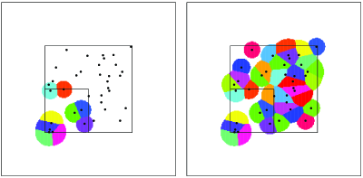
Figure 2: Concept of exhausting sequences: start with a small cube and repeatedly double its edge lengths to exhaust space [cost function $c(x,y)=|x-y|^{2}$].

For $n\in\mathbb{N}_{0}:=\mathbb{N}\cup\{0\}$ and $z\in\mathbb{Z}^{d}$ define the cube or box $B_{n}(z)$ of generation $n$ with basepoint $z$ by

$$B_{n}(z)=z+\bigl{[}0,2^{n}\bigr{)}^{d}.$$

For $z=0$ simply put $B_{n}=B_{n}(0)$. More generally, for $\gamma=(\gamma_{k})\in\Gamma:=(\{0,1\}^{d})^{\mathbb{N}}$ put

$$B_{n}(z,\gamma)=z-\sum_{k=1}^{n}2^{k-1}\gamma_{k}+\bigl{[}0,2^{n}\bigr{)}^{d}.$$

Starting with the unit box $B_{0}(z,\gamma)=z+[0,1)^{d}$, for any random vector $\gamma\in\Gamma$ the sequence $(B_{n}(z,\gamma))_{n\in\mathbb{N}_{0}}$ can be constructed iteratively as follows: Given the box $B_{n}(z,\gamma)$ attach $2^{d}-1$ copies of it—depending on the random variable $\gamma_{n+1}=(\gamma_{n+1}^{1},\ldots,\gamma_{n+1}^{d})$ with values in $\{0,1\}^{d}$—either on the right (if $\gamma_{n+1}^{1}=0$) or on the left (if $\gamma_{n+1}^{1}=1$), either on the backside (if $\gamma_{n+1}^{2}=0$) of on the front (if $\gamma_{n+1}^{2}=1$), either on the top (if $\gamma_{n+1}^{3}=0$) or on the bottom (if $\gamma_{n+1}^{3}=1$), etc; see Figure 2.

The sequence $(B_{n}(z,\gamma))_{n\in\mathbb{N}_{0}}$ for fixed $z$ and $\gamma$ is increasing and for $\nu$-almost every $\gamma\in\Gamma$ it increases to $\mathbb{R}^{d}$. Each of the boxes $B_{n}(z,\gamma)$ contains the point $z$.

Put

$${\mathfrak{c}}_{n}:=2^{-dn}\cdot\mathbb{E}[\mathsf{C}_{B_{n}(z,\gamma)}].$$

Note that translation invariance (equivariance plus stationarity) implies that the right-hand side does not depend on $z\in\mathbb{Z}^{d}$ and $\gamma\in\Gamma$.

Corollary 2.3

(i) The sequence $({\mathfrak{c}}_{n})_{n\in\mathbb{N}_{0}}$ is nondecreasing. The limit

$${\mathfrak{c}}_{\infty}=\lim_{n\to\infty}{\mathfrak{c}}_{n}=\sup_{n}{\mathfrak{c}}_{n}$$

exists in $(0,\infty]$. [(iii)]

Assume that $\mu^{\bullet}$ is ergodic. Then, we have for all $z\in\mathbb{Z}^{d}$, for all $\gamma\in\Gamma$ and for $\mathbb{P}$-almost every $\omega\in\Omega$,

$$\liminf_{n\to\infty}2^{-nd}\mathsf{C}_{B_{n}(z,\gamma)}(\omega)={\mathfrak{c}}_{\infty}.$$

$\mathfrak{c}_{\infty}\leq\inf_{q\in\Pi_{s}}\mathfrak{C}_{\infty}(q)$ where $\Pi_{s}$ denotes the set of semicouplings of $\mathfrak{L}$ and $\mu^{\bullet}$.

(i) is an immediate consequence of the previous lemma. For (ii) fix an arbitrary nested sequence of boxes $(B_{n})_{n}$ generated by a standard exhaustion. Then we have by superadditivity $\forall\omega\in\Omega$ for all $n,k\in\mathbb{N}$

$$2^{-d(n+k)}\mathsf{C}_{B_{n+k}}(\omega)\geq 2^{-dk}\sum_{j=1}^{2^{dk}}2^{-nd}\mathsf{C}_{B_{n}^{j}}(\omega),$$

where $B_{n}^{j}$ are disjoint copies of $B_{n}$ such that $\bigcup_{j=1}^{2^{dk}}B_{n}^{j}=B_{n+k}$. In the limit of $k\to\infty$ we get by ergodicity for $\mathbb{P}$-a.e. $\omega$

$$\liminf_{k\to\infty}2^{-kd}\mathsf{C}_{B_{k}}(\omega)\geq\mathbb{E}\bigl{[}2^{-nd}\mathsf{C}_{B_{n}}\bigr{]}={\mathfrak{c}}_{n}$$

for each $n\in\mathbb{N}$ and thus

$$\liminf_{k\to\infty}2^{-kd}\mathsf{C}_{B_{k}}(\omega)\geq{\mathfrak{c}}_{\infty}.$$

On the other hand, Fatou’s lemma implies

$$\mathbb{E}\Bigl{[}\liminf_{n\to\infty}2^{-nd}\mathsf{C}_{B_{n}}\Bigr{]}\leq\liminf_{n\to\infty}\mathbb{E}\bigl{[}2^{-nd}\mathsf{C}_{B_{n}}\bigr{]}={\mathfrak{c}}_{\infty}.$$

Both inequalities together imply the assertion.

For (iii) take any semicoupling $q^{\bullet}$ of $\mathfrak{L}$ and $\mu^{\bullet}\mathbb{P}$. Then we have for any n

$$2^{-dn}\mathfrak{Cost}\bigl{(}1_{R^{d}\times B_{n}\times\Omega}q^{\bullet}\bigr{)}\geq\mathfrak{c}_{n}.$$

Taking the limit yields

$$\mathfrak{C}_{\infty}\bigl{(}q^{\bullet}\bigr{)}=\liminf_{n\to\infty}2^{-dn}\mathfrak{Cost}\bigl{(}1_{R^{d}\times B_{n}\times\Omega}q^{\bullet}\bigr{)}\geq\lim_{n}\mathfrak{c}_{n}=\mathfrak{c}_{\infty}.$$

Corollary 2.4

$\mathfrak{c}_{\infty}$ only depends on the scale $\vartheta$ and on the distribution of $\mu^{\bullet}$, not on the choice of the realization of $\mu^{\omega}$ on a particular probability space $(\Omega,\mathfrak{A},\mathbb{P})$.

It is sufficient to show that $\mathfrak{c}_{n}$ just depends on the distribution of $\mu^{\bullet}$. For a given set of points $\mathchar 260\relax(\omega)$ in $B_{n}$ there is a unique semicoupling $q^{\omega}_{B_{n}}$ of $\mathfrak{L}$ and $1_{B_{n}}\mu^{\omega}$ minimizing $\mathsf{Cost}$; see Proposition 6.3. Hence, $q^{\omega}_{B_{n}}$ just depends on $\mathchar 260\relax(\omega)$. However, the distribution of the points in $B_{n}$, $\mathchar 260\relax(\omega)$, just depends on the distribution of $\mu^{\bullet}$.

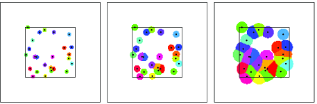
Figure 3: Semicoupling of Lebesgue and 25 points in the cube with $c(x,y)=|x-y|$ where each point gets mass $1/9,1/3,1$, respectively.

Remark 2.5.

None of the previous definitions and results required that $\mu^{\bullet}$ have subunit intensity. However, one easily verifies that

$$\beta>1\quad\Longrightarrow\quad{\mathfrak{c}}_{\infty}=\infty,$$

where $\beta:=\mathbb{E}[\mu^{\bullet}([0,1)^{d})]$ denotes the intensity of the equivariant point process.

Remark 2.6.

The problem of finding an optimal semicoupling between $\mathfrak{L}$ and a Poisson point process $\mu^{\bullet}$ of intensity $\beta<1$ is equivalent to the problem of finding an optimal semicoupling between $\mathfrak{L}$ and $\beta\cdot\hat{\mu}^{\bullet}$ where $\hat{\mu}^{\bullet}$ is a Poisson point process of unit intensity; see Figure 3.

Indeed, given $\beta\in(0,1)$ and a semicoupling $q^{\bullet}$ of $\mathfrak{L}$ and a Poisson point process $\mu^{\bullet}$ of intensity $\beta$. Put $\tau\dvtx x\mapsto\beta^{1/d}x$ on $\mathbb{R}^{d}$ as well as on $\mathbb{R}^{d}\times\mathbb{R}^{d}$. Then $\hat{\mu}^{\omega}:=\tau_{*}\mu^{\omega}$ is a Poisson point process with intensity 1, and

$$\tilde{q}^{\omega}:=\beta\cdot\tau_{*}q^{\omega}$$

is a semicoupling of $\mathfrak{L}$ and $\beta\cdot\hat{\mu}^{\omega}$. Conversely, given any Poisson point process $\hat{\mu}^{\omega}$ of unit intensity and any semicoupling $\tilde{q}^{\omega}$ of $\mathfrak{L}$ and $\beta\cdot\hat{\mu}^{\omega}$, then $q^{\omega}:=\frac{1}{\beta}\cdot(\tau^{-1})_{*}\tilde{q}^{\omega}$ is a semicoupling of $\mathfrak{L}$ and $\mu^{\omega}:=(\tau^{-1})_{*}\hat{\mu}^{\omega}$, the latter being a Poisson point process of intensity $\beta$. In both cases, $q$ is equivariant if and only if $\tilde{q}$ is equivariant.

The asymptotic mean transportation cost for $\tilde{q}^{\bullet}$ measured with scale $\vartheta$ will coincide with the asymptotic mean transportation cost for $q^{\bullet}$ measured with scale $\vartheta_{\beta}(r):=\beta\cdot\vartheta(\beta^{-1/d}r)$,

$$\mathbb{E}\int_{\mathbb{R}^{d}\times[0,1)^{d}}\vartheta\bigl{(}|x-y|\bigr{)}\,d\tilde{q}^{\bullet}=\mathbb{E}\int_{\mathbb{R}^{d}\times[0,1)^{d}}\vartheta_{\beta}\bigl{(}|x-y|\bigr{)}\,dq^{\bullet}.$$

3 Uniqueness

Throughout this section we fix an equivariant point process $\mu^{\bullet}\dvtx\Omega\to\mathcal{M}(\mathbb{R}^{d})$ of subunit intensity and with finite asymptotic mean transportation cost $\mathfrak{c}_{\infty}$.

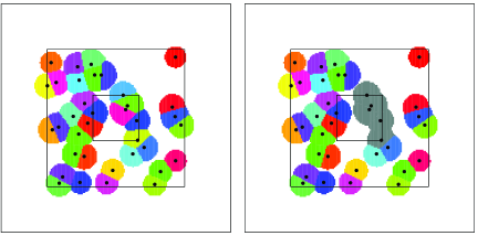
Figure 4: The left picture is a semicoupling of Lebesgue and 36 points with cost function $c(x,y)=|x-y|^{4}$. In the right picture, the five points within the small cube can choose new partners from the mass that was transported to them in the left picture (corresponding to the measure $\lambda_{A}$). If the semicoupling on the left-hand side is locally optimal, then the points in the small cube on the right-hand side will choose from the gray region exactly the partners they have in the left picture.

Proposition 3.1

Given a counting measure $\mu\in\mathcal{N}(\mathbb{R}^{d})$ and a semicoupling $q$ of $\mathfrak{L}$ and $\mu$, then the following properties are equivalent: [(iii)]

For each bounded Borel set $A\subset\mathbb{R}^{d}$, the measure $1_{\mathbb{R}^{d}\times A}q$ is the unique optimal semicoupling of the measures $\lambda_{A}(\cdot):=q(\cdot,A)$ and $1_{A}\mu$; see Figure 4.

The support of $q$ is $c$-cyclically monotone, more precisely,

$$\sum_{i=1}^{n}c(x_{i},y_{i})\leq\sum_{i=1}^{n}c(x_{i},y_{i+1})$$

for any $n\in\mathbb{N}$ and any choice of points $(x_{1},y_{1}),\ldots,(x_{n},y_{n})$ in $\mathrm{supp}(q)$ with the convention $y_{n+1}=y_{1}$; cf. (3).

There exists a density $\rho\dvtx\mathbb{R}^{d}\to[0,1]$ and a $c$-cyclically monotone map $T^{\omega}\dvtx\{\rho>0\}\to\mathbb{R}^{d}$ such that

$$q=(\mathrm{id},T)_{*}(\rho\mathfrak{L}).$$ (4)

Recall that, by definition, a map $T$ is $c$-cyclically monotone if and only if the closure of its graph $\{(x,T(x))\dvtx x\in A^{\omega}\}$ is a $c$-cyclically monotone set.

The implications $\mathrm{(iii)}\Longrightarrow\mathrm{(ii)}\Longrightarrow\mathrm{(i)}$ follow from Lemma 6.1.

$\mathrm{(i)}\Longrightarrow\mathrm{(iii)}$: Fix an exhaustion $(B_{n}^{\prime})_{n}$ of $\mathbb{R}^{d}$ by boxes, say $B_{n}^{\prime}=[-2^{n-1},\break 2^{n-1})^{d}$. For each $n\in\mathbb{N}$, let $\rho_{n}$ be the density of the measure $\lambda_{n}:=\lambda_{B_{n}^{\prime}}$ on $\mathbb{R}^{d}$. This is the part of Lebesgue measure from which the points inside of $B_{n}^{\prime}$ might choose their “partners.” Obviously, $0\leq\rho_{n}\leq\rho_{n+1}\leq 1.$ Hence, $\lim_{n\to\infty}\rho_{n}(x)=\rho(x)\leq 1$ exists $\mathfrak{L}$-a.e.

Assuming (i), according to Proposition 6.3 (or, more precisely, a canonical extension of it for semicouplings of $\rho\mathfrak{L}$ and $\sigma$), there exists a $c$-cyclically monotone map $T_{n}\dvtx\{\rho_{n}>0\}\to\mathbb{R}^{d}$ such that

$$dq(x,y)=d\delta_{T_{n}(x)}(y)\rho_{n}(x)\,d\mathfrak{L}(x)\qquad\mbox{on }\mathbb{R}^{d}\times B_{n}^{\prime}.$$

Since the left-hand side is independent of $n$, we have

$$T_{n+1}=T_{n}\qquad\mbox{on }\{\rho_{n}>0\}.$$

This trivially yields the existence of

$$T:=\lim_{n\to\infty}T_{n}\qquad\mbox{on }\{\rho>0\}:=\lim_{n\to\infty}\{\rho_{n}\},$$

defining a $c$-cyclically monotone map $T\dvtx\{\rho>0\}\to\mathbb{R}^{d}$ with the property that

$$dq(x,y)=d\delta_{T(x)}(y)\rho(x)\,d\mathfrak{L}(x).$$

Remark 3.2.

Set $A=\{\rho>0\}.$ In the sequel, any transport map $T\dvtx A\to\mathbb{R}^{d}$ as above will be extended to a map $T\dvtx\mathbb{R}^{d}\to\mathbb{R}^{d}\cup\{\eth\}$ by putting $T(x):=\eth$ for all $x\in\mathbb{R}^{d}\setminus A$ where $\eth$ denotes an isolated point added to $\mathbb{R}^{d}$ (“point at infinity,” “cemetery”). Then (4) simplifies to

$$q=(\mathrm{id},T)_{*}(\rho\mathfrak{L})\qquad\mbox{on }\mathbb{R}^{d}\times\mathbb{R}^{d}.$$ (5)

Moreover, we put $c(x,T(x))=c(x,\eth):=0$ for $x\in\mathbb{R}^{d}\setminus A$.

Definition 3.3.

• A semicoupling $Q=q^{\bullet}\mathbb{P}$ of $\mathfrak{L}$ and $\mu^{\bullet}$ is called locally optimal if and only if some (hence every) of the properties of the previous proposition are satisfied for $\mathbb{P}$-a.e. $\omega\in\Omega$.

• A semicoupling $Q=q^{\bullet}\mathbb{P}$ of $\mathfrak{L}$ and $\mu^{\bullet}$ is called asymptotically optimal if and only if

  $$\liminf_{n\to\infty}2^{-nd}\mathfrak{Cost}(1_{\mathbb{R}^{d}\times B_{n}^{\prime}}Q)=\mathfrak{c}_{\infty}$$

  for some exhaustion $(B_{n}^{\prime})_{n}$ of $\mathbb{R}^{d}$ by boxes $B_{n}^{\prime}=B_{n}(z,\gamma)$.

• A semicoupling $Q=q^{\bullet}\mathbb{P}$ of $\mathfrak{L}$ and $\mu^{\bullet}$ is called equivariant if and only if for each $z\in\mathbb{Z}^{d}$ the measure $Q$ is equivariant under the diagonal action of $\mathbb{Z}^{d}$, that is,

  $$q^{\omega}(A,B)=q^{\omega+z}(A+z,B+z)$$

  for all $z\in\mathbb{Z}^{d}$ and $A,B\in\mathcal{B}(\mathbb{R}^{d}).$

• A semicoupling $Q=q^{\bullet}\mathbb{P}$ of $\mathfrak{L}$ and $\mu^{\bullet}$ is called optimal if and only if it is equivariant and asymptotically optimal.

The very same definitions apply to couplings instead of semicouplings.

Remark 3.4.

(i) Asymptotic optimality is not sufficient for uniqueness and it does not imply local optimality: Given any asymptotically optimal semicoupling $q^{\bullet}$ and a bounded Borel set $A\subset\mathbb{R}^{d}$ of positive volume, choose an arbitrary coupling $\tilde{q}_{A}^{\omega}$ of the measures $q^{\omega}(\cdot,A)$ and $1_{A}\mu^{\omega}$, which are the marginals of $q_{A}^{\omega}:=1_{\mathbb{R}^{d}\times A}q^{\omega}$. If $\mu^{\omega}(A)\geq 2$ (which happens with positive probability), then one can always achieve that $\tilde{q}_{A}^{\omega}$ is a nonoptimal coupling and that it is different from $q_{A}^{\omega}$. Put

$$\tilde{q}^{\omega}:=q^{\omega}+\tilde{q}_{A}^{\omega}-q_{A}^{\omega}.$$

Then $\tilde{q}^{\bullet}$ is an asymptotically optimal semicoupling of $\mathfrak{L}$ and $\mu^{\bullet}$. It is not locally optimal and it does not coincide with $q^{\bullet}$. [(iii)]

Local optimality does not imply asymptotic optimality and it is not sufficient for uniqueness: For instance in the case $p=2$, given any coupling $q^{\bullet}$ of $\mathfrak{L}$ and $\mu^{\bullet}$ and $z\in\mathbb{R}^{d}\setminus\{0\}$, then

$$d\tilde{q}^{\omega}(x,y):=dq^{\omega}(x+z,y)$$

defines another locally optimal coupling of $\mathfrak{L}$ and $\mu^{\bullet}$. At most one of them can be asymptotically optimal.

Note that local optimality—in contrast to asymptotic optimality and equivariance—is not preserved under convex combinations. We do not claim that local optimality and asymptotic optimality imply uniqueness.

Local optimality links classical optimal transportation problems, problems between finite measures, with optimal transportation problems between $\mathfrak{L}$ and a point process by locally optimizing the semicouplings.

Given $\gamma,\eta\in\mathcal{M}(\mathbb{R}^{d})$ with $\gamma(\mathbb{R}^{d})\geq\eta(\mathbb{R}^{d})$, we define the transportation cost by

$$\mathsf{Cost}(\gamma,\eta):=\inf\bigl{\{}\mathsf{Cost}(q)\dvtx q\in\Pi_{s}(\gamma,\eta)\bigr{\}}.$$

Similarly, given measure valued random variables $\gamma^{\bullet},\eta^{\bullet}\dvtx\Omega\to\mathcal{M}(\mathbb{R}^{d})$ and a bounded Borel set $A\subset\mathbb{R}^{d}$ we define the mean transportation cost by

$$\mathfrak{Cost}\bigl{(}\gamma^{\bullet},\eta^{\bullet}\bigr{)}:=\inf\bigl{\{}\mathfrak{Cost}\bigl{(}q^{\bullet}\mathbb{P}\bigr{)}\dvtx q^{\omega}\in\Pi_{s}\bigl{(}\gamma^{\omega},\eta^{\omega}\bigr{)}\mbox{ for a.e. }\omega\bigr{\}}.$$

Given a (semi-) coupling $Q=q^{\bullet}\mathbb{P}$ of $\mathfrak{L}$ and $\mu^{\bullet}\mathbb{P}$, recall the definition of $\lambda_{A}^{\bullet}$ from Proposition 3.1. We define the efficiency of the (semi-) coupling $Q$ on the set $A$ by

$$\mathfrak{eff}_{A}(Q):=\frac{\mathfrak{Cost}(\lambda^{\bullet}_{A},1_{A}\mu^{\bullet})}{\mathfrak{Cost}(1_{\mathbb{R}^{d}\times A}Q)}.$$

It is a number in $(0,1]$. The (semi-) coupling $Q$ is said to be efficient on $A$ if and only if $\mathfrak{eff}_{A}(Q)=1$. Otherwise, it is inefficient on $A$.

Lemma 3.5

(i) $Q$ is locally optimal if and only if $\mathfrak{eff}_{A}(Q)=1$ for all bounded Borel sets $A\subset\mathbb{R}^{d}$. [(ii)]

$\mathfrak{eff}_{A}(Q)=1$ for some $A\subset\mathbb{R}^{d}$ implies $\mathfrak{eff}_{A^{\prime}}(Q)=1$ for all $A^{\prime}\subset A$.

(i) Let $A$ be given and $\omega\in\Omega$ be fixed. Then $1_{\mathbb{R}^{d}\times A}q^{\omega}$ is the optimal semicoupling of the measures $\lambda^{\omega}_{A}$ and $1_{A}\mu^{\omega}$ if and only if

$$\mathsf{Cost}\bigl{(}1_{\mathbb{R}^{d}\times A}q^{\omega}\bigr{)}=\mathsf{Cost}\bigl{(}\lambda_{A}^{\omega},1_{A}\mu^{\omega}\bigr{)}.$$ (6)

On the other hand, $\mathfrak{eff}_{A}(Q)=1$ is equivalent to

$$\mathbb{E}\bigl{[}\mathsf{Cost}\bigl{(}1_{\mathbb{R}^{d}\times A}q^{\bullet}\bigr{)}\bigr{]}=\mathbb{E}\bigl{[}\mathsf{Cost}\bigl{(}\lambda_{A}^{\bullet},1_{A}\mu^{\omega}\bigr{)}\bigr{]}.$$

The latter, in turn, is equivalent to (6) for $\mathbb{P}$-a.e. $\omega\in\Omega$.[(ii)]

If the transport $q$ restricted to $\mathbb{R}^{d}\times A$ is optimal, then also each of its sub-transports; see Theorem 4.6 in villani2009optimal . ∎

Theorem 3.6

Every optimal semicoupling of $\mathfrak{L}$ and $\mu^{\bullet}\mathbb{P}$ is locally optimal.

Assume we are given a semicoupling $Q$ of $\mathfrak{L}$ and $\mu^{\bullet}\mathbb{P}$ which is equivariant and not locally optimal. According to the previous lemma, the latter implies that there exist $n\in\mathbb{N}$ and $z_{0}\in\mathbb{Z}^{d}$ such that the semicoupling $Q$ is not efficient on the box $B_{n}(z_{0})=z_{0}+[0,2^{n})^{d}$, that is,

$$\eta:=\mathfrak{eff}_{B_{n}(z_{0})}(Q)<1.$$

By equivariance this implies $\mathfrak{eff}_{B_{n}(z)}(Q)=\eta<1$ for all $z\in\mathbb{Z}^{d}$. Hence, for each $z\in\mathbb{Z}^{d}$ there exists a measure-valued random variable $\tilde{q}^{\bullet}_{B_{n}(z)}$ such that $\tilde{q}^{\omega}_{B_{n}(z)}$ for a.e. $\omega$ is a semicoupling of $\lambda^{\omega}_{B_{n}(z)}$ and $1_{B_{n}(z)}\mu^{\omega}$ and more efficient than $q^{\omega}_{B_{n}(z)}:=1_{\mathbb{R}^{d}\times{B_{n}(z)}}\cdot q^{\omega}$, that is, such that

$$\mathbb{E}\bigl{[}\mathsf{Cost}\bigl{(}\tilde{q}^{\bullet}_{B_{n}(z)}\bigr{)}\bigr{]}\leq\eta\cdot\mathbb{E}\bigl{[}\mathsf{Cost}\bigl{(}q^{\bullet}_{B_{n}(z)}\bigr{)}\bigr{]}.$$

Put

$$\tilde{q}^{\bullet}:=\sum_{z\in(2^{n}\mathbb{Z})^{d}}\tilde{q}^{\bullet}_{B_{n}(z)}.$$

Then $\tilde{q}^{\bullet}$ is a semicoupling of $\mathfrak{L}$ and $\mu^{\bullet}$ and for all $z\in(2^{n}\mathbb{Z})^{d}$

$$\mathbb{E}\bigl{[}\mathsf{Cost}\bigl{(}1_{\mathbb{R}^{d}\times{B_{n}(z)}}\tilde{q}^{\bullet}\bigr{)}\bigr{]}\leq\eta\cdot\mathbb{E}\bigl{[}\mathsf{Cost}\bigl{(}1_{\mathbb{R}^{d}\times{B_{n}(z)}}q^{\bullet}\bigr{)}\bigr{]}.$$

Equivariance of $q^{\bullet}$—together with uniqueness of cost minimizers on bounded sets—implies equivariance of $\tilde{q}^{\bullet}$ under the group $(2^{n}\mathbb{Z}^{d})$. In other words, $\tilde{Q}=\tilde{q}^{\bullet}\mathbb{P}$ is an $(2^{n}\mathbb{Z}^{d})$-equivariant semicoupling of $\mathfrak{L}$ and $\mu^{\bullet}\mathbb{P}$ which satisfies

$$\mathfrak{Cost}(1_{\mathbb{R}^{d}\times B_{n}(z)}\tilde{Q})\leq\eta\cdot\mathfrak{Cost}(1_{\mathbb{R}^{d}\times B_{n}(z)}Q)$$

for all $z\in(2^{n}\mathbb{Z})^{d}$. Additivity of the mean cost functional $\mathfrak{Cost}(\cdot)$ implies

$$\mathfrak{Cost}(1_{\mathbb{R}^{d}\times B_{n+k}}\tilde{Q})\leq\eta\cdot\mathfrak{Cost}(1_{\mathbb{R}^{d}\times B_{n+k}}Q)$$

for all $k\in\mathbb{N}_{0}$ and therefore, due to Corollary 2.3(iii), finally

$$\mathfrak{c}_{\infty}\leq\liminf_{k\to\infty}\mathfrak{Cost}(1_{\mathbb{R}^{d}\times B_{k}}\tilde{Q})\leq\eta\cdot\liminf_{k\to\infty}\mathfrak{Cost}(1_{\mathbb{R}^{d}\times B_{k}}Q)$$

with $\eta<1$. This proves that $Q$ is not asymptotically optimal.

Lemma 3.7

Let $q^{\omega}=(\mathrm{id},T^{\omega})_{*}(\rho^{\omega}\mathfrak{L})$ be an optimal semicoupling between $\mathfrak{L}$ and $\mu^{\bullet}.$ Then, $\mathbb{P}$-a.s. we have $\rho^{\omega}(x)\in\{0,1\}\mathfrak{L}$-a.e.

Assume there is a $n\in\mathbb{N}$ and $B_{n}(z_{0})=z_{0}+[0,2^{n})^{d}$ such that on a set of positive $\mathbb{P}$-measure

$$q^{\omega}_{n}:=1_{\mathbb{R}^{d}\times B_{n}(z_{0})}\,dq^{\omega}(x,y)=\bigl{(}\mathrm{id},T^{\omega}\bigr{)}_{*}\bigl{(}\rho_{n}^{\omega}\mathfrak{L}\bigr{)}$$

with $0<\rho^{\omega}_{n}<1$ on a set of positive $\mathfrak{L}$-measure. However, due to Proposition 6.3 this implies that $Q=q^{\bullet}\mathbb{P}$ is not efficient on $B_{n}(z_{0})$ because it is possible to construct a semicoupling between $1_{\rho_{n}^{\omega}>0}\mathfrak{L}$ and $1_{B_{n}(z_{0})}\mu^{\omega}$ with less cost. By the same reasoning as in the last proof, this implies that $Q$ is not optimal.

Hence, any optimal semicoupling can be written as $q^{\omega}=(\mathrm{id},T^{\omega})_{*}\mathfrak{L}$ for some measurable map $T\dvtx A^{\omega}\to\mathbb{R}^{d}\cup\{\eth\}$; cf Remark 3.2.

Theorem 3.8

There exists at most one optimal semicoupling of $\mathfrak{L}$ and $\mu^{\bullet}\mathbb{P}$.

Assume we are given two optimal semicouplings $q_{1}^{\bullet}$ and $q_{2}^{\bullet}$. Then also $q^{\bullet}:=\frac{1}{2}q_{1}^{\bullet}+\frac{1}{2}q_{2}^{\bullet}$ is an optimal semicoupling. Hence, by the previous theorem all three couplings—$q_{1}^{\bullet}$, $q_{2}^{\bullet}$ and $q^{\bullet}$—are locally optimal. Thus, for a.e. $\omega$ by the results of Proposition 3.1 and the last lemma there exist maps $T_{1}^{\omega},T_{2}^{\omega},T^{\omega}$ and sets $A_{1}^{\omega},A_{2}^{\omega},A^{\omega}$ such that

$$dq^{\omega}(x,y) = d\delta_{T^{\omega}(x)}(y)1_{A^{\omega}}(x)\,d\mathfrak{L}(x)$$

$$= \bigl{(}\tfrac 12d\delta_{T_{1}^{\omega}(x)}(y)1_{A^{\omega}_{1}}(x)+\tfrac 12d\delta_{T_{2}^{\omega}(x)}(y)1_{A^{\omega}_{2}}(x)\bigr{)}\,d\mathfrak{L}(x).$$

This, however, implies $T_{1}^{\omega}(x)=T_{2}^{\omega}(x)$ for a.e. $x\in A_{1}^{\omega}\cap A_{2}^{\omega}$ and, moreover, $A_{1}^{\omega}=A_{2}^{\omega}$. Thus $q_{1}^{\omega}=q_{2}^{\omega}$.

Remark 3.9.

Note that we only used equivariance under the action of $\mathbb{Z}^{d}$. However, the minimizer is equivariant under the action of $\mathbb{R}^{d}$. For the uniqueness it would also have been sufficient to require equivariance under the action of $k\mathbb{Z}^{d}$ for some $k\in\mathbb{N}$.

Theorem 3.10

(i) If $\mu^{\bullet}$ has unit intensity, then every optimal semicoupling of $\mathfrak{L}$ and $\mu^{\bullet}$ is indeed a coupling of them. [(ii)]

Conversely, if an optimal coupling exists, then $\mu^{\bullet}$ must have unit intensity.

This theorem is in a similar spirit as Theorem 4 in stable-marriage . (i) Let $Q$ be an optimal semicoupling. For $n\in\mathbb{N}$ put $B_{n}(z)=z+[0,2^{n})^{d}$ and consider the saturation $\alpha_{k}:=2^{-kd}Q(B_{k}(z)\times B_{k}(z)\times\Omega)\leq 1$. Note that $\alpha_{k}$ is independent of $z\in\mathbb{Z}^{d}$. Hence, we have $\alpha_{k}\leq\alpha_{k+1}$. Indeed, $B_{k+1}(z)$ is the disjoint union of $2^{d}$ cubes $B_{k}(y_{j})$ for suitable $y_{j}$. Therefore,

$$\alpha_{k+1}\geq 2^{-d}\sum_{j=1}^{2^{d}}2^{-kd}Q\bigl{(}B_{k}(y_{j})\times B_{k}(y_{j})\times\Omega\bigr{)}=\alpha_{k}.$$

Thus, the limit $\alpha_{\infty}:=\lim_{k\to\infty}\alpha_{k}$ exists, and we have $\alpha_{\infty}\in(0,1]$.

Since $\mu^{\bullet}$ has unit intensity and since $Q$ is a semicoupling, we have $Q(\mathbb{R}^{d}\times B_{k}\times\Omega)=2^{kd}$. Let us first assume that $\alpha_{\infty}<1$ and choose $r=[(1+\frac{1}{2}(1-\alpha_{\infty}))^{1/d}-1]/2$. Then for all $k\in\mathbb{N}$ mass of a total amount of at least $(1-\alpha_{\infty})2^{kd}$ has to be transported from $\complement B_{k}$ into $B_{k}$. The volume of the $(r2^{k})$-neighborhood of the box $B_{k}$ is less than $\frac{1}{2}(1-\alpha_{\infty})2^{kd}$. Hence, mass of total amount of at least $\frac{1}{2}(1-\alpha_{\infty})2^{kd}$ has to be transported at least the distance $r2^{k}$. Thus, we can estimate the costs per unit from below by

$$2^{-kd}\int_{\mathbb{R}^{d}\times B_{k}\times\Omega}c(x,y)\,dQ(x,y,\omega)\geq\frac{1}{2}(1-\alpha_{\infty})\vartheta\bigl{(}r2^{k}\bigr{)}.$$

The right-hand side diverges as $k$ tends to infinity which contradicts the finiteness of the costs per unit. Thus, we have $\alpha_{\infty}=1$. Furthermore, for all $k$ there is a $u\in B_{k}(0)$ such that

$$\alpha_{k} = 2^{-kd}Q\bigl{(}B_{k}(0)\times B_{k}(0)\times\Omega\bigr{)}$$

$$= 2^{-kd}\sum_{v\in B_{k}(0)\cap\mathbb{Z}^{d}}Q\bigl{(}B_{0}(v)\times B_{k}(0)\times\Omega\bigr{)}$$

$$\leq Q\bigl{(}B_{0}(u)\times B_{k}(0)\times\Omega\bigr{)}\leq Q\bigl{(}B_{0}(u)\times\mathbb{R}^{d}\times\Omega\bigr{)}.$$

However, by translation invariance (equivariance plus stationarity) the quantity $Q(B_{0}(u)\times\mathbb{R}^{d}\times\Omega)$ is independent of $u$. Moreover, it is bounded above by 1 as $Q$ is a semicoupling. Hence, we have for all $v\in\mathbb{R}^{d}$:

$$1=\limsup_{k\to\infty}\alpha_{k}\leq Q\bigl{(}B_{0}(v)\times\mathbb{R}^{d}\times\Omega\bigr{)}\leq 1.$$

Therefore, $Q$ is actually a coupling of the Lebesgue measure and the point process.

(ii) Assume that $Q$ is an optimal coupling and that $\beta<1$. Then a similar argumentation as above yields that for each box $B_{k}$, Lebesgue measure of total mass $\geq(1-\beta)\cdot 2^{kd}$ has to be transported from the interior of $B_{k}$ to the exterior. As $k$ tends to $\infty$, the costs of these transports explode.

Corollary 3.11

In the case $\vartheta(r)=r^{2}$, given an optimal coupling $q^{\bullet}$ of $\mathfrak{L}$ and a point process $\mu^{\bullet}$ of unit intensity then for a.e. $\omega\in\Omega$ there exists a convex function $\varphi^{\omega}\dvtx\mathbb{R}^{d}\to\mathbb{R}$ (unique up to additive constants) such that

$$q^{\omega}=\bigl{(}\mathrm{id},\nabla\varphi^{\omega}\bigr{)}_{*}\mathfrak{L}.$$

In particular, a “fair allocation rule” is given by the monotone map $T^{\omega}=\nabla\varphi^{\omega}$.

Moreover, for a.e. $\omega$ and any center $\xi\in\Xi(\omega):=\mathrm{supp}(\mu^{\omega})$, the associated cell

$$S^{\omega}(\xi)={\bigl{(}T^{\omega}\bigr{)}^{-1}\bigl{(}\{\xi\}\bigr{)}}$$

is a convex polyhedron of volume $\mu^{\omega}(\xi)\in\mathbb{N}$. If the point process is simple, then all these cells have volume 1.

By Proposition 3.1 we know that $T^{\omega}=\lim_{n\to\infty}T_{n}^{\omega}$, where $T_{n}^{\omega}$ is an optimal transportation map from some set $A_{n}^{\omega}$ to $B_{n}^{\prime}$. From the classical theory (see Brenier , GangboMcCann1996 ), we know that $T_{n}^{\omega}=\nabla\varphi_{n}^{\omega}$ for some convex function $\varphi_{n}^{\omega}$. More precisely,

$$\varphi_{n}^{\omega}(x)=\max_{\xi\in\mathchar 260\relax(\omega)\cap B_{n}^{\prime}}\bigl{(}x^{2}-|x-\xi|^{2}/2+b_{\xi}\bigr{)}$$

for some constants $b_{\xi}$. Moreover, we know that $T_{n+k}^{\omega}=T_{n}^{\omega}$ on $A_{n}^{\omega}$ for any $k\in\mathbb{N}$. Fix any $\xi_{0}\in\Xi(\omega)$. Then there is $n\in\mathbb{N}$ such that $\xi_{0}\in B_{n}^{\prime}$. Then $(T_{n+k}^{\omega})^{-1}(\xi_{0})=(T_{n}^{\omega})^{-1}(\xi_{0})$ for any $k\in\mathbb{N}$. Furthermore,

$$T_{n}^{\omega}(x)=\xi_{0}\quad\Leftrightarrow\quad-|x-\xi_{0}|^{2}/2+b_{\xi_{0}}>-|x-\xi|^{2}/2+b_{\xi}$$

$$\eqntext{\forall\xi\in\Xi(\omega)\cap B_{n}^{\prime},\xi\neq\xi_{0}.}$$ (7)

For fixed $\xi\neq\xi_{0}$ this equation describes two half-spaces separated by a hyperplane (defined by equality in the equation above). The set $S^{\omega}(\xi_{0})$ is then given as the intersection of all these halfspaces defined by $\xi_{0}$ and $\xi\in\Xi(\omega)\cap B_{n}^{\prime}$. Hence, it is a convex polytope. Moreover, the last inequality is exactly the defining equation for a Laguerre tessellation wrt $\operatorname{supp}(\mu^{\omega})$ and weights $b_{\xi}$; see lautensack2007 .

4 Construction of optimal semicouplings

Again we fix an equivariant point process $\mu^{\bullet}\dvtx\Omega\to\mathcal{M}(\mathbb{R}^{d})$ of subunit intensity and with finite asymptotic mean transportation cost $\mathfrak{c}_{\infty}$.

4.1 Second randomization and annealed limits

The crucial step in our construction of an optimal coupling of Lebesgue measure and the point process will be the introduction of a second randomization, in addition to the first randomness modeled on the probability space $(\Omega,\mathfrak{A},\mathbb{P})$ which describes the random choice $\omega\mapsto\mu^{\omega}$ of a realization of the point process. The second randomization describes the random choice $\gamma\mapsto(B_{n}(z,\gamma))_{n\in\mathbb{N}}$ of an increasing sequence of boxes containing a given starting point $z\in\mathbb{Z}^{d}$; see also Section 2.7. It is modeled on the Bernoulli scheme $(\Gamma,\mathfrak{B}(\Gamma),\nu)$ with $\Gamma=(\{0,1\}^{d})^{\mathbb{N}}$, $\mathfrak{B}(\Gamma)$ its Borel $\sigma$-field and $\nu$ the uniform distribution on $\Gamma=(\{0,1\}^{d})^{\mathbb{N}}$ (or, more precisely, the infinite product of the uniform distribution on $\{0,1\}^{d}$).

For each $z\in\mathbb{Z}^{d},\gamma\in\Gamma$ and $k\in\mathbb{N}$, recall that $Q_{B_{k}(z,\gamma)}$ denotes the minimizer of $\mathfrak{Cost}$ among the semicouplings of $\mathfrak{L}$ and $(1_{B_{k}(z,\gamma)}\mu^{\bullet})\mathbb{P}$ as constructed in Theorem 2.1. Equivariance of this minimizer implies that

$$Q_{B_{k}(z^{\prime},\gamma)}(A,B,\omega)=Q_{B_{k}(z,\gamma)}\bigl{(}A+z-z^{\prime},B+z-z^{\prime},\omega+z-z^{\prime}\bigr{)}$$

for all $z,z^{\prime}\in\mathbb{Z}^{d}$ and $A,B\in\mathcal{B}(M)$. Put

$$dQ_{z}^{k}(x,y,\omega):=\int_{\Gamma}\,dQ_{B_{k}(z,\gamma)}(x,y,\omega)\,d\nu(\gamma)$$

and $d\dot{Q}_{z}^{k}(x,y,\omega):=1_{B_{0}(z)}(y)\,dQ_{z}^{k}(x,y,\omega)$.

The measure $\dot{Q}_{z}^{k}$ defines a semicoupling between the Lebesgue measure and the point process restricted to the box $B_{0}(z)$. It is a deterministic, fractional allocation in the following sense:

• it is a deterministic function of $\mu^{\omega}$ and does not depend on any additional randomness [coming, e.g., from $d\nu(\gamma$)];

• the measure transported into a given point of the point process has density $\leq 1$.

The last fact of course implies that the semicoupling $\dot{Q}_{z}^{k}$ is not optimal. The first fact implies that all the objects derived from $\dot{Q}_{z}^{k}$ in the sequel—like $\dot{Q}_{z}^{\infty}$ and $Q^{\infty}$—are also deterministic.

Lemma 4.1

(i) For each $k\in\mathbb{N}$ and $z\in\mathbb{Z}^{d}$

$$\int_{\mathbb{R}^{d}\times B_{0}(z)\times\Omega}c(x,y)\,dQ_{z}^{k}(x,y,\omega)\leq{\mathfrak{c}_{\infty}}.\vspace*{-6pt}$$

[(iii)]

The family $(\dot{Q}_{z}^{k})_{k\in\mathbb{N}}$ of probability measures on $\mathbb{R}^{d}\times\mathbb{R}^{d}\times\Omega$ is relatively compact in the weak topology.

There exist probability measures $\dot{Q}_{z}^{\infty}$ and a subsequence $(k_{l})_{l\in\mathbb{N}}$ such that for all $z\in\mathbb{Z}^{d}$

$$\dot{Q}^{k_{l}}_{z}\longrightarrow\dot{Q}_{z}^{\infty}\qquad\mbox{weakly as $l\to\infty$.}$$

(i) Let us fix $z\in\mathbb{Z}^{d}$ and start with the following important observation: For given $n\in\mathbb{N}$ the initial box $B_{0}(z)$ has each possible “relative position within $B_{n}(z,\gamma)$” with equal probability.

Hence, together with translation invariance of $Q_{B_{k}(z,\gamma)}$ (which in turn follows from equivariance and stationarity of $\mathbb{P}$) we obtain

$$\int_{\mathbb{R}^{d}\times B_{0}(z)\times\Omega}c(x,y)\,dQ_{z}^{k}(x,y,\omega)$$

$$\qquad=\int_{\Gamma}\int_{\mathbb{R}^{d}\times B_{0}(z)\times\Omega}c(x,y)\,dQ_{B_{k}(z,\gamma)}(x,y,\omega)\,d\nu(\gamma)$$

$$\qquad=2^{-kd}\sum_{v\in B_{k}(z)\cap\mathbb{Z}^{d}}\biggl{[}\int_{\mathbb{R}^{d}\times B_{0}(v)\times\Omega}c(x,y)\,dQ_{B_{k}(z)}(x,y,\omega)\biggr{]}$$

$$\qquad=2^{-kd}\int_{\mathbb{R}^{d}\times B_{k}(z)\times\Omega}c(x,y)\,dQ_{B_{k}(z)}(x,y,\omega)$$

$$\qquad={\mathfrak{c}}_{k}\leq{\mathfrak{c}}_{\infty}.$$

(ii) In order to prove tightness of $(\dot{Q}_{z}^{k})_{k\in\mathbb{N}}$, let

$$K_{m}:=\Bigl{\{}y\in\mathbb{R}^{d}\dvtx\inf_{x\in B_{0}(z)}|x-y|\leq m\Bigr{\}}$$

denote the closed $m$-neighborhood of the unit box based at $z$. Then

$$Q_{z}^{k}\bigl{(}\complement K_{m}\times B_{0}(z)\times\Omega\bigr{)}\leq\frac{1}{\vartheta(m)}\int_{\mathbb{R}^{d}\times B_{0}(z)\times\Omega}c(x,y)\,dQ_{z}^{k}(x,y,\omega)\leq\frac{1}{\vartheta(m)}\cdot{\mathfrak{c}}_{\infty}.$$

Since $\vartheta(m)\to\infty$ as $m\to\infty$ this proves tightness of the family $(\dot{Q}_{z}^{k})_{k\in\mathbb{N}}$ on $\mathbb{R}^{d}\times\mathbb{R}^{d}\times\Omega$. (Recall that $\Omega$ was assumed to be compact from the very beginning.)

(iii) Tightness yields the existence of $\dot{Q}_{z}^{\infty}$ and of a converging subsequence for each $z$. A standard argument (“diagonal sequence”) then gives convergence for all $z\in\mathbb{Z}^{d}$ along a common subsequence.

Lemma 4.2

(i) For each $r>0$ there exist numbers $\varepsilon_{k}(r)$ with $\varepsilon_{k}(r)\to 0$ as $k\to\infty$ such that for all $z,z^{\prime}\in\mathbb{Z}^{d}$ and all $k\in\mathbb{N}$

$$\int_{\Gamma}Q_{B_{k}(z^{\prime},\gamma)}(A)\,d\nu(\gamma)$$

$$\qquad\leq\int_{\Gamma}Q_{B_{k}(z,\gamma)}(A)\,d\nu(\gamma)+\varepsilon_{k}\bigl{(}\bigl{|}z-z^{\prime}\bigr{|}\bigr{)}\cdot\sup_{\gamma}Q_{B_{k}(z^{\prime},\gamma)}(A)$$

for any Borel set $A\subset\mathbb{R}^{d}\times\mathbb{R}^{d}\times\Omega$.

(ii) For all $z_{1},\ldots,z_{m}\in\mathbb{Z}^{d}$, all $k\in\mathbb{N}$ and all Borel sets $A\subset\mathbb{R}^{d}$,

$$\sum_{i=1}^{m}\dot{Q}_{z_{i}}^{k}\bigl{(}A\times\mathbb{R}^{d}\times\Omega\bigr{)}\leq\Biggl{(}1+\sum_{i=1}^{m}\varepsilon_{k}\bigl{(}|z_{1}-z_{i}|\bigr{)}\Biggr{)}\cdot\mathfrak{L}(A).$$

(i) First, note that for each $z,z^{\prime}\in\mathbb{Z}^{d},k\in\mathbb{N},\gamma\in\Gamma$,

$$z^{\prime}\in B_{k}(z,\gamma)\quad\iff\quad\exists\gamma^{\prime}\dvtx B_{k}(z,\gamma)=B_{k}\bigl{(}z^{\prime},\gamma^{\prime}\bigr{)}$$

and in this case

$$\nu\bigl{(}\bigl{\{}\gamma^{\prime}\dvtx B_{k}\bigl{(}z^{\prime},\gamma^{\prime}\bigr{)}=B_{k}(z,\gamma)\bigr{\}}\bigr{)}=2^{-kd}.$$

Moreover,

$$\nu\bigl{(}\bigl{\{}\gamma\dvtx z^{\prime}\notin B_{k}(z,\gamma)\bigr{\}}\bigr{)}\leq\varepsilon_{k}\bigl{(}\bigl{|}z-z^{\prime}\bigr{|}\bigr{)}$$

for some $\varepsilon_{k}(r)$ with $\varepsilon_{k}(r)\to 0$ as $k\to\infty$ for each $r>0$. It implies that for each pair $z,z^{\prime}\in\mathbb{Z}^{d}$ and each $k\in\mathbb{N}$,

$$\nu\bigl{(}\bigl{\{}\gamma\in\Gamma\dvtx\exists\gamma^{\prime}\dvtx B_{k}(z,\gamma)=B_{k}\bigl{(}z^{\prime},\gamma^{\prime}\bigr{)}\bigr{\}}\bigr{)}\geq 1-\varepsilon_{k}\bigl{(}\bigl{|}z-z^{\prime}\bigr{|}\bigr{)}.$$

Therefore, for each Borel set $A\subset\mathbb{R}^{d}\times\mathbb{R}^{d}\times\Omega$,

$$\int_{\Gamma}Q_{B_{k}(z^{\prime},\gamma)}(A)\,d\nu(\gamma)$$

$$\qquad\leq\int_{\Gamma}Q_{B_{k}(z,\gamma)}(A)\,d\nu(\gamma)+\varepsilon_{k}\bigl{(}\bigl{|}z-z^{\prime}\bigr{|}\bigr{)}\cdot\sup_{\gamma}Q_{B_{k}(z^{\prime},\gamma)}(A).$$

(ii) According to the previous part (i), for each Borel set $A\subset\mathbb{R}^{d}$,

$$\sum_{i=1}^{m}\dot{Q}^{k}_{z_{i}}\bigl{(}A\times\mathbb{R}^{d}\times\Omega\bigr{)}$$

$$\qquad=\sum_{i=1}^{m}\int_{\Gamma}Q_{B_{k}(z_{i},\gamma)}\bigl{(}A\times B_{0}(z_{i})\times\Omega\bigr{)}\,d\nu(\gamma)$$

$$\qquad\leq\sum_{i=1}^{m}\biggl{[}\int_{\Gamma}Q_{B_{k}(z_{1},\gamma)}\bigl{(}A\times B_{0}(z_{i})\times\Omega\bigr{)}\,d\nu(\gamma)$$

$$\hskip 16.0pt\qquad\quad{}+\varepsilon_{k}\bigl{(}|z_{1}-z_{i}|\bigr{)}\cdot\sup_{\gamma\in\Gamma}Q_{B_{k}(z_{i},\gamma)}\bigl{(}A\times B_{0}(z_{i})\times\Omega\bigr{)}\biggr{]}$$

$$\qquad\leq Q_{B_{k}(z_{1},\gamma)}\bigl{(}A\times\mathbb{R}^{d}\times\Omega\bigr{)}+\sum_{i=1}^{m}\varepsilon_{k}\bigl{(}|z_{1}-z_{i}|\bigr{)}\cdot\mathfrak{L}(A)$$

$$\qquad\leq\Biggl{(}1+\sum_{i=1}^{m}\varepsilon_{k}\bigl{(}|z_{1}-z_{i}|\bigr{)}\Biggr{)}\cdot\mathfrak{L}(A).$$

Theorem 4.3

The measure $Q^{\infty}:=\sum_{z\in\mathbb{Z}^{d}}\dot{Q}_{z}^{\infty}$ is an optimal semicoupling of $\mathfrak{L}$ and $\mu^{\bullet}$.

(i) Second/third marginal: For any $f\in\mathcal{C}_{b}^{+}(\mathbb{R}^{d}\times\Omega)$ we have due to Lemma 4.1,

$$\int_{\mathbb{R}^{d}\times\Omega}f(y,\omega)\,dQ^{\infty}(x,y,\omega)$$

$$\qquad=\sum_{z\in\mathbb{Z}^{d}}\int_{\mathbb{R}^{d}\times\Omega}f(y,\omega)\,d\dot{Q}_{z}^{\infty}(x,y,\omega)$$

$$\qquad=\sum_{z\in\mathbb{Z}^{d}}\lim_{l\to\infty}\int_{\mathbb{R}^{d}\times\Omega}f(y,\omega)\,d\dot{Q}^{k_{l}}_{z}(x,y,\omega)$$

$$\qquad=\sum_{z\in\mathbb{Z}^{d}}\int_{\mathbb{R}^{d}\times\Omega}f(y,\omega)1_{B_{0}(z)}(y)\,d\bigl{(}\mu^{\bullet}\mathbb{P}\bigr{)}(y,\omega)$$

$$\qquad=\int_{\mathbb{R}^{d}\times\Omega}f(y,\omega)\,d\bigl{(}\mu^{\bullet}\mathbb{P}\bigr{)}(y,\omega).$$

(ii) First marginal: Let an arbitrary bounded open set $A\subset\mathbb{R}^{d}$ be given, and let $(z_{i})_{i\in\mathbb{N}}$ be an enumeration of $\mathbb{Z}^{d}$. According to the previous Lemma 4.2, for any $m\in\mathbb{N}$ and any $k\in\mathbb{N}$,

$$\sum_{i=1}^{m}\dot{Q}_{z_{i}}^{k}\bigl{(}A\times\mathbb{R}^{d}\times\Omega\bigr{)}\leq\Biggl{(}1+\sum_{i=1}^{m}\varepsilon_{k}\bigl{(}|z_{1}-z_{i}|\bigr{)}\Biggr{)}\cdot\mathfrak{L}(A).$$

Letting first $k$ tend to $\infty$ yields

$$\sum_{i=1}^{m}\dot{Q}_{z_{i}}^{\infty}\bigl{(}A\times\mathbb{R}^{d}\times\Omega\bigr{)}\leq\mathfrak{L}(A).$$

Then with $m\to\infty$ we obtain

$$Q^{\infty}\bigl{(}A\times\mathbb{R}^{d}\times\Omega\bigr{)}\leq\mathfrak{L}(A),$$

which proves that $(\pi_{1})_{*}Q^{\infty}\leq\mathfrak{L}$.

(iii) Optimality: By construction, $Q^{\infty}$ is $\mathbb{Z}^{d}$-equivariant. Due to the stationarity of $\mathbb{P}$, the asymptotic cost is given by

$$\int_{\mathbb{R}^{d}\times B_{0}(0)\times\Omega}c(x,y)\,dQ^{\infty}(x,y,\omega)$$

$$\qquad=\sum_{z\in\mathbb{Z}^{d}}\int_{\mathbb{R}^{d}\times B_{0}(0)\times\Omega}c(x,y)\,d\dot{Q}_{z}^{\infty}(x,y,\omega)$$

$$\qquad=\int_{\mathbb{R}^{d}\times B_{0}(0)\times\Omega}c(x,y)\,d\dot{Q}_{0}^{\infty}(x,y,\omega)\leq\mathfrak{c}_{\infty}.$$

Here the final inequality is due to Lemma 4.1, property (i) (which remains true in the limit $k=\infty$), and the last equality comes from the fact that

$$\int_{\mathbb{R}^{d}\times B_{0}(u)\times\Omega}c(x,y)\,d\dot{Q}_{z}^{k}(x,y,\omega)=0$$

for all $z\not=u$ and for all $k\in\mathbb{N}$ (which also remains true in the limit $k=\infty$).

Corollary 4.4

(i) For $k\to\infty$, the sequence of measures $Q^{k}:=\break\sum_{z\in\mathbb{Z}^{d}}\dot{Q}^{k}_{z}$, $k\in\mathbb{N}$, converges vaguely to the unique optimal semicoupling $Q^{\infty}$.

[(ii)]

For each $z\in\mathbb{Z}^{d}$ the sequence $(Q^{k}_{z})_{k\in\mathbb{N}}$ converges vaguely to the unique optimal semicoupling $Q^{\infty}$.

(i) A slight extension of the previous Lemma 4.1(iii)${}+{}$Theorem 4.3 yields that each subsequence $(Q^{k_{n}})_{n}$ of the above sequence $(Q^{k})_{k}$ will have a sub-subsequence converging vaguely to an optimal coupling of $\mathfrak{L}$ and $\mu^{\bullet}$. Since the optimal coupling is unique, all these limit points coincide. Hence, the whole sequence $(Q^{k})_{k}$ converges to this limit point; see, for example, dudley2002real , Proposition 9.3.1.

(ii) Lemma 4.2(i) implies that for $z,z^{\prime},u\in\mathbb{Z}^{d}$ and every measurable $A\subset\mathbb{R}^{d}\times\mathbb{R}^{d}\times\Omega$,

$$\bigl{|}Q_{z}^{k}\bigl{(}A\cap\bigl{(}\mathbb{R}^{d}\times B_{0}(u)\times\Omega\bigr{)}\bigr{)}-Q_{z^{\prime}}^{k}\bigl{(}A\cap\bigl{(}\mathbb{R}^{d}\times B_{0}(u)\times\Omega\bigr{)}\bigr{)}\bigr{|}$$

$$\qquad\leq\varepsilon_{k}\bigl{(}\bigl{|}z-z^{\prime}\bigr{|}\bigr{)}\cdot\sup_{v\in\mathbb{Z}^{d}}Q_{B_{k}(v)}\bigl{(}A\cap\bigl{(}\mathbb{R}^{d}\times B_{0}(u)\times\Omega\bigr{)}\bigr{)}$$

$$\qquad\leq\varepsilon_{k}\bigl{(}\bigl{|}z-z^{\prime}\bigr{|}\bigr{)}\to 0$$

as $k\to\infty$. Hence, for each $f\in\mathcal{C}_{c}(\mathbb{R}^{d}\times\mathbb{R}^{d}\times\Omega)$ and each $z^{\prime}\in\mathbb{R}^{d}$,

$$\biggl{|}\sum_{z\in\mathbb{Z}^{d}}\int f(x,y,\omega)1_{B_{0}(z)}(y)\,dQ_{z}^{k}-\int f(x,y,\omega)\,dQ^{k}_{z^{\prime}}\biggr{|}\to 0.$$

That is, $|\int f\,dQ^{k}-\int f\,dQ^{k}_{z^{\prime}}|\to 0$ as $k\to\infty$.

Corollary 4.5

We have $\mathfrak{c}_{\infty}=\inf_{q^{\bullet}\in\Pi_{s}}\mathfrak{C}_{\infty}(q^{\bullet})$ where $\Pi_{s}$ denotes the set of all semicouplings $q^{\bullet}$ of $\mathfrak{L}$ and $\mu^{\bullet}$. In particular, the following holds:

$$\inf_{q^{\bullet}\in\Pi_{s}}\liminf_{n\to\infty}\frac{1}{\mathfrak{L}(B_{n})}\mathbb{E}\biggl{[}\int_{\mathbb{R}^{d}\times B_{n}}c(x,y)\,dq^{\bullet}(x,y)\biggr{]}$$

$$\qquad=\liminf_{n\to\infty}\inf_{q^{\bullet}\in\Pi_{s}}\frac{1}{\mathfrak{L}(B_{n})}\mathbb{E}\biggl{[}\int_{\mathbb{R}^{d}\times B_{n}}c(x,y)\,dq^{\bullet}(x,y)\biggr{]}.$$

The optimal coupling $Q$ constructed in the previous theorem has mean asymptotic transportation cost bounded above by $\mathfrak{c}_{\infty}$. Thus, we have $\inf_{q^{\bullet}\in\Pi_{s}}\mathfrak{C}_{\infty}(q^{\bullet})\leq\mathfrak{c}_{\infty}$. Together with Lemma 2.3, this yields the claim.

4.2 Quenched limits

According to Section 3, the unique optimal semicoupling between $d\mathfrak{L}(x)$ and $d\mu^{\omega}(y)\,d\mathbb{P}(\omega)$ can be represented on $\mathbb{R}^{d}\times\mathbb{R}^{d}\times\Omega$ as

$$dQ^{\infty}(x,y,\omega)=d\delta_{T(x,\omega)}(y)\,d\mathfrak{L}(x)\,d\mathbb{P}(\omega)$$

by means of a measurable map

$$T\dvtx\mathbb{R}^{d}\times\Omega\to\mathbb{R}^{d}\cup\{\eth\},$$

defined uniquely almost everywhere. Similarly, for each $z\in Z^{d}$ and $k\in\mathbb{N}$, there exists a measurable map

$$T_{z,k}\dvtx\mathbb{R}^{d}\times\Omega\times\Gamma\to\mathbb{R}^{d}\cup\{\eth\}$$

such that for each $\gamma\in\Gamma$ the measure

$$dQ_{B_{k}(z,\gamma)}(x,y,\omega)=d\delta_{T_{z,k}(x,\omega,\gamma)}(y)\,d\mathfrak{L}(x)\,d\mathbb{P}(\omega)$$

on $\mathbb{R}^{d}\times\mathbb{R}^{d}\times\Omega$ is the unique optimal semicoupling between $d\mathfrak{L}(x)$ and $1_{B_{k}(z,\gamma)}(y)\,d\mu^{\omega}(y)\,d\mathbb{P}(\omega)$.

Proposition 4.6

For every $z\in Z^{d}$,

$$T_{z,k}(x,\omega,\gamma)\to T(x,\omega)\qquad\mbox{as }k\to\infty\mbox{ locally in }\mathfrak{L}\otimes\mathbb{P}\otimes\nu\mbox{-measure}.$$

The claim basically relies on the following lemma which is a slight modification (and extension) of a result in Ambrosio-ln-ot .

Lemma 4.7

Let $X,Y$ be locally compact Polish spaces, $\theta$ a Radon measure on $X$ and $\rho$ a metric on $Y$ compatible with the topology. [(ii)]

For all $n\in\mathbb{N}$ let $T_{n},T\dvtx X\to Y$ be Borel measurable maps. Put$dQ_{n}(x,y):=d\delta_{T_{n}(x)}(y)\,d\theta(x)$ and $dQ(x,y):=d\delta_{T(x)}(y)\,d\theta(x)$. Then

$$T_{n}\to T\mbox{ locally in measure on }X\quad\Longleftrightarrow\quad Q_{n}\to Q\mbox{ vaguely in }\mathcal{M}(X\times Y).$$

More generally, let $T$ and $Q$ be as before whereas

$$dQ_{n}(x,y):=\int_{X^{\prime}}\,d\delta_{T_{n}(x,x^{\prime})}(y)\,d\theta^{\prime}\bigl{(}x^{\prime}\bigr{)}\,d\theta(x)$$

for some probability space $(X^{\prime},\mathfrak{A}^{\prime},\theta^{\prime})$ and suitable measurable maps $T_{n}\dvtx X\times X^{\prime}\to Y$. Then

$$Q_{n}\to Q\mbox{ vaguely in }\mathcal{M}(X\times Y)$$

$$\qquad\Longrightarrow\quad T_{n}\bigl{(}x,x^{\prime}\bigr{)}\to T(x)\mbox{ locally in measure on }X\times X^{\prime}.$$

(i) Assume $T_{n}\to T$ in $\theta$-measure. Then also $f\circ(\mathrm{id},T_{n})\to f\circ(\mathrm{id},T)$ in $\theta$-measure for any $f\in C_{c}(X\times Y)$. Therefore, by the dominated convergence theorem we have

$$\int f(x,y)\,dQ_{n}=\int f\bigl{(}x,T_{n}(x)\bigr{)}\,d\theta\to\int f\bigl{(}x,T(x)\bigr{)}\,d\theta=\int f(x,y)\,dQ.$$

This proves the vague convergence of $Q_{n}$ toward Q.

For the opposite direction, fix $\tilde{K}\subset X$ compact and $\varepsilon>0$. By Lusin’s theorem there is a compact set $K\subset\tilde{K}$ such that $T|_{K}$ is continuous and $\theta(\tilde{K}\setminus K)<\varepsilon$. Put $\eta\dvtx\mathbb{R}_{+}\to\mathbb{R}_{+},t\mapsto 1\wedge|t|/\varepsilon$. The function

$$\phi(x,y)=1_{K}(x)\eta\bigl{(}\rho\bigl{(}y,T(x)\bigr{)}\bigr{)}$$

is upper semicontinuous, nonnegative and compactly supported. Thus, there exist $\phi_{l}\in C_{c}(X\times Y)$ with $\phi_{l}\searrow\phi$. By assumption, we have for each $l$

$$\int\phi(x,y)\,dQ_{n}(x,y)\leq\int\phi_{l}(x,y)\,dQ_{n}(x,y)\stackrel{{\scriptstyle n\to\infty}}{{\to}}\int\phi_{l}(x,y)\,dQ(x,y).$$

Moreover,

$$\int\phi_{l}(x,y)\,dQ(x,y)\stackrel{{\scriptstyle l\to\infty}}{{\to}}\int\phi(x,y)\,dQ(x,y)=0.$$

Therefore, $\lim_{n\to\infty}\int\phi(x,y)\,dQ_{n}(x,y)=0$. In other words,

$$\lim_{n\to\infty}\int 1_{K}(x)\eta\bigl{(}\rho\bigl{(}T_{n}(x),T(x)\bigr{)}\bigr{)}\,d\theta(x)=0.$$

This implies $\lim_{n\to\infty}\theta(\{x\in K\dvtx\rho(T_{n}(x),T(x))\geq\varepsilon\})=0$ and then in turn

$$\lim_{n\to\infty}\theta\bigl{(}\bigl{\{}x\in\tilde{K}\dvtx\rho\bigl{(}T_{n}(x),T(x)\bigr{)}\geq 2\varepsilon\bigr{\}}\bigr{)}=0.$$

(ii) Given any compact $\tilde{K}\subset X$ and any $\varepsilon>0$, choose $\phi$ as before. Then vague convergence again implies $\lim_{n\to\infty}\int\phi(x,y)\,dQ_{n}(x,y)=0$. This, in other words, now reads as

$$\lim_{n\to\infty}\int_{X}\int_{X^{\prime}}1_{K}(x)\eta\bigl{(}\rho\bigl{(}T_{n}\bigl{(}x,x^{\prime}\bigr{)},T(x)\bigr{)}\bigr{)}\,d\theta^{\prime}\bigl{(}x^{\prime}\bigr{)}\,d\theta(x)=0.$$

Therefore,

$$\lim_{n\to\infty}\bigl{(}\theta\otimes\theta^{\prime}\bigr{)}\bigl{(}\bigl{\{}\bigl{(}x,x^{\prime}\bigr{)}\in\tilde{K}\times X^{\prime}\dvtx\rho\bigl{(}T_{n}\bigl{(}x,x^{\prime}\bigr{)},T(x)\bigr{)}\geq 2\varepsilon\bigr{\}}\bigr{)}=0.$$

This is the claim. Proof of Proposition 4.6 Fix $z\in Z^{d}$ and recall that

$$Q_{z}^{k}\to Q^{\infty}\qquad\mbox{vaguely on }\mathbb{R}^{d}\times\mathbb{R}^{d},$$

where

$$dQ^{\infty}(x,y,\omega)=d\delta_{T(x,\omega)}(y)\,d\mathfrak{L}(x)\,d\mathbb{P}(\omega)$$

and

$$dQ_{z}^{k}(x,y,\omega) = \int_{\Gamma}\,dQ_{B_{k}(z,\gamma)}(x,y,\omega)\,d\nu(\gamma)$$

$$= \int_{\Gamma}\,d\delta_{T_{z,k}(x,\omega,\gamma)}(y)\,d\mathfrak{L}(x)\,d\mathbb{P}(\omega)\,d\nu(\gamma)$$

with transport maps $T\dvtx\mathbb{R}^{d}\times\Omega\to\mathbb{R}^{d}\cup\{\eth\}$ and $T_{z,k}\dvtx\mathbb{R}^{d}\times\Omega\times\Gamma\to\mathbb{R}^{d}\cup\{\eth\}$ as above. Apply assertion (ii) of the previous lemma with $X:=\mathbb{R}^{d}\times\Omega,X^{\prime}=\Gamma,Y=\mathbb{R}^{d}\cup\{\eth\}$ and $\theta=\mathfrak{L}\otimes\mathbb{P},\theta^{\prime}=\nu$.

Actually, this convergence result can significantly be improved.

Theorem 4.8

For every $z\in Z^{d}$ and every bounded Borel set $M\subset\mathbb{R}^{d}$,

$$\lim_{k\to\infty}(\mathfrak{L}\otimes\mathbb{P}\otimes\nu)\bigl{(}\bigl{\{}(x,\omega,\gamma)\in M\times\Omega\times\Gamma\dvtx T_{z,k}(x,\omega,\gamma)\not=T(x,\omega)\bigr{\}}\bigr{)}=0.$$

Let $M$ as above and $\varepsilon>0$ be given. Finiteness of the asymptotic mean transportation cost implies that there exists a bounded set $M^{\prime}\subset\mathbb{R}^{d}$ such that

$$(\mathfrak{L}\otimes\mathbb{P})\bigl{(}\bigl{\{}(x,\omega)\in M\times\Omega\dvtx T(x,\omega)\notin M^{\prime}\bigr{\}}\bigr{)}\leq\varepsilon.$$

Given the bounded set $M^{\prime}$ there exists $\delta>0$ such that the probability to find two distinct particles of the point process at distance $<\delta$, at least one of them within $M^{\prime}$, is less than $\varepsilon$, that is,

$$\mathbb{P}\bigl{(}\bigl{\{}\omega\dvtx\exists\bigl{(}y,y^{\prime}\bigr{)}\in M^{\prime}\times\mathbb{R}^{d}\dvtx 0<\bigl{|}y-y^{\prime}\bigr{|}<\delta,\mu^{\omega}\bigl{(}\{y\}\bigr{)}>0,\mu^{\omega}\bigl{(}\bigl{\{}y^{\prime}\bigr{\}}\bigr{)}>0\bigr{\}}\bigr{)}\leq\varepsilon.$$

On the other hand, Proposition 4.6 states that with high probability the maps $T$ and $T_{z,k}$ have distance less than $\delta$. More precisely, for each $\delta>0$ there exists $k_{0}$ such that for all $k\geq k_{0}$,

$$(\mathfrak{L}\otimes\mathbb{P}\otimes\nu)\bigl{(}\bigl{\{}(x,\omega,\gamma)\in M\times\Omega\times\Gamma\dvtx\bigl{|}T_{z,k}(x,\omega,\gamma)-T(x,\omega)\bigr{|}\geq\delta\bigr{\}}\bigr{)}\leq\varepsilon.$$

Since all the maps $T$ and $T_{z,k}$ take values in the support of the point process (plus the point $\eth$) it follows that

$$(\mathfrak{L}\otimes\mathbb{P}\otimes\nu)\bigl{(}\bigl{\{}(x,\omega,\gamma)\in M\times\Omega\times\Gamma\dvtx T_{z,k}(x,\omega,\gamma)\not=T(x,\omega)\bigr{\}}\bigr{)}\leq 3\varepsilon$$

for all $k\geq k_{0}$.

Corollary 4.9

There exists a subsequence $(k_{l})_{l}$ such that

$$T_{z,k_{l}}(x,\omega,\gamma)\to T(x,\omega)\qquad\mbox{as }l\to\infty$$

for almost every $x\in\mathbb{R}^{d}$, $\omega\in\Omega$, $\gamma\in\Gamma$ and every $z\in Z^{d}$. Indeed, the sequence $(T_{z,k_{l}})_{l}$ is finally stationary. That is, there exists a random variable $l_{z}\dvtx\mathbb{R}^{d}\times\Omega\times\Gamma\to\mathbb{N}$ such that almost surely

$$T_{z,k_{l}}(x,\omega,\gamma)=T(x,\omega)\qquad\mbox{for all }l\geq l_{z}(x,\omega,\gamma).$$

Corollary 4.10

There is a measurable map $\Upsilon\dvtx\mathcal{M}(\mathbb{R}^{d})\to\mathcal{M}(\mathbb{R}^{d}\times\mathbb{R}^{d})$ s.t. $q^{\omega}:=\Upsilon(\mu^{\omega})$ denotes the unique optimal semicoupling between $\mathfrak{L}$ and $\mu^{\omega}$. In particular the optimal semicoupling is a factor coupling.

By Theorem 2.1, the maps $T_{z,k}$ are measurable with respect to the sigma algebra generated by $\mu^{\bullet}$. By Theorem 4.8, the optimal transportation map $T$ is also measurable with respect to the sigma algebra generated by $\mu^{\bullet}$. Because the optimal semicoupling $q^{\bullet}$ is given by $q^{\omega}=(\mathrm{id},T^{\omega})_{*}\mathfrak{L}$, it is also measurable with respect to the sigma algebra generated by $\mu^{\bullet}$. Thus there is a measurable map $\Upsilon$ such that $q^{\bullet}=\Upsilon(\mu^{\bullet})$.

5 Estimates for the asymptotic mean transportation cost of a Poisson process

Throughout this section, $\mu^{\bullet}$ will be a Poisson point process of intensity $\beta\leq 1$. The asymptotic mean transportation cost for $\mu^{\bullet}$ will be denoted by

$$\mathfrak{c}_{\infty}=\mathfrak{c}_{\infty}(\vartheta,d,\beta)$$

or, if $\vartheta(r)=r^{p}$, by $\mathfrak{c}_{\infty}(p,d,\beta)$. We will present sufficient as well as necessary conditions for finiteness of $\mathfrak{c}_{\infty}$. These criteria will be quite sharp. Moreover, in the case of $L^{p}$-cost, we also present explicit sharp estimates for $\mathfrak{c}_{\infty}$.

To begin with, let us summarize some elementary monotonicity properties of $\mathfrak{c}_{\infty}(\vartheta,d,\beta)$.

Lemma 5.1

(i) $\vartheta\leq\overline{\vartheta}$ implies $\mathfrak{c}_{\infty}(\vartheta,d,\beta)\leq\mathfrak{c}_{\infty}(\overline{\vartheta},d,\beta)$.

More generally, $\limsup_{r\to\infty}\frac{\overline{\vartheta}(r)}{\vartheta(r)}<\infty$ and $\mathfrak{c}_{\infty}(\vartheta,d,\beta)<\infty$ imply $\mathfrak{c}_{\infty}(\overline{\vartheta},d,\break\beta)<\infty$. [(iii)]

If $\overline{\vartheta}=\varphi\circ\vartheta$ for some convex increasing $\varphi\dvtx\mathbb{R}_{+}\to\mathbb{R}_{+}$, then

$$\varphi\bigl{(}\beta^{-1}\mathfrak{c}_{\infty}(\vartheta,d,\beta)\bigr{)}\leq\beta^{-1}\mathfrak{c}_{\infty}(\overline{\vartheta},d,\beta).$$

$\beta\leq\overline{\beta}$ implies $\mathfrak{c}_{\infty}(\vartheta,d,\beta)\leq\mathfrak{c}_{\infty}(\vartheta,d,\overline{\beta})$.

(i) Is obvious. (ii) If $\overline{q}$ denotes the optimal semicoupling for $\overline{\vartheta}$, then Jensen’s inequality implies

$$\beta^{-1}\mathfrak{c}_{\infty}(\overline{\vartheta},d,\beta)$$

$$\qquad=\beta^{-1}\mathbb{E}\int_{\mathbb{R}^{d}\times[0,1)^{d}}\varphi\bigl{(}\vartheta\bigl{(}|x-y|\bigr{)}\bigr{)}\,d\overline{q}(x,y)$$

$$\qquad\geq\varphi\biggl{(}\beta^{-1}\mathbb{E}\int_{\mathbb{R}^{d}\times[0,1)^{d}}\vartheta\bigl{(}|x-y|\bigr{)}\,d\overline{q}(x,y)\biggr{)}\geq\varphi\bigl{(}\beta^{-1}\mathfrak{c}_{\infty}(\vartheta,d,\beta)\bigr{)}.$$

(iii) Given a realization $\overline{\mu}^{\omega}$ of a Poisson point process with intensity $\overline{\beta}$. Delete each point $\xi\in\operatorname{supp}[\overline{\mu}^{\omega}]$ with probability $1-\beta/\overline{\beta}$, independently of each other. Then the remaining point process $\mu^{\omega}$ is a Poisson point process with intensity $\beta$. Hence, each semicoupling $\overline{q}^{\omega}$ between $\mathfrak{L}$ and $\overline{\mu}^{\omega}$ leads to a semicoupling $q^{\omega}$ between $\mathfrak{L}$ and $\mu^{\omega}$ with less or equal transportation cost. The centers which survive are coupled with the same cells as before.

5.1 Lower estimates

Theorem 5.2 ((holroyd2001find ))

Assume $\beta=1$ and $d\leq 2$. Then for all translation invariant couplings of Lebesgue and Poisson

$$\mathbb{E}\biggl{[}\int_{\mathbb{R}^{d}\times[0,1)^{d}}|x-y|^{d/2}\,dq^{\bullet}(x,y)\biggr{]}=\infty.$$

Theorem 5.3

For all $\beta\leq 1$ and $d\geq 1$ there exists a constant $\kappa^{\prime}=\kappa^{\prime}(d,\beta)$ such that for all translation invariant semicouplings of Lebesgue and Poisson

$$\mathbb{E}\biggl{[}\int_{\mathbb{R}^{d}\times[0,1)^{d}}\exp\bigl{(}\kappa^{\prime}|x-y|^{d}\bigr{)}\,dq^{\bullet}(x,y)\biggr{]}=\infty.$$

The result is well known in the case $\beta=1$. In this case, it is based on a lower bound for the event “no Poisson particle in the cube $[-r,r)^{d}$” and on a lower estimate for the cost of transporting the Lebesgue measure in $[-r/2,r/2)^{d}$ to some distribution on $\mathbb{R}^{d}\setminus[-r,r)^{d}$,

$$\mathfrak{c}_{\infty}\geq\exp\bigl{(}-(2r)^{d}\bigr{)}\cdot\vartheta\biggl{(}\frac{r}{2}\biggr{)}\cdot 2^{-d}.$$

Hence, $\mathfrak{c}_{\infty}\to\infty$ as $r\to\infty$ if $\vartheta(r)=\exp(\kappa^{\prime}r^{d})$ with $\kappa^{\prime}>2^{2d}$.

However, this argument breaks down in the case $\beta<1$. We will present a different argument which works for all $\beta\leq 1$.

Consider the event “more than $(3r)^{d}$ Poisson particles in the box $[-r/2,r/2)^{d}$” or, formally,

$$\Omega(r)=\bigl{\{}\mu^{\bullet}\bigl{(}[-r/2,r/2)^{d}\bigr{)}\geq(3r)^{d}\bigr{\}}.$$

Note that $\mathbb{E}\mu^{\bullet}([-r/2,r/2)^{d})=\beta r^{d}$ with $\beta\leq 1$. For $\omega\in\Omega(r)$, the cost of a semicoupling between $\mathfrak{L}$ and $1_{[-r/2,r/2)^{d}}\mu^{\omega}$ is bounded from below by

$$\vartheta(r/2)\cdot r^{d}$$

(since $r^{d}$ Poisson points—or more—must be transported at least a distance $r/2$). The large deviation result formulated in the next lemma allows us to estimate

$$\mathbb{P}\bigl{(}\Omega(r_{n})\bigr{)}\geq e^{-k\cdot{r_{n}}^{d}}$$

for any $k>I_{\beta}(3^{d})$ and suitable $r_{n}\to\infty$. Hence, if $\vartheta(r)\geq\exp(\kappa^{\prime}r^{d})$ with $\kappa^{\prime}>2^{d}\cdot k$, then

$$\mathfrak{c}_{\infty}\geq\mathbb{P}\bigl{(}\Omega(r_{n})\bigr{)}\cdot\vartheta(r/2)\geq\exp\bigl{(}\bigl{(}\kappa^{\prime}2^{-d}-k\bigr{)}r^{d}\bigr{)}\to\infty$$

as $r\to\infty$.

Lemma 5.4

Given any nested sequence of boxes $B_{n}(z,\gamma)\subset\mathbb{R}^{d}$ and $t\geq\beta$

$$\lim_{n\to\infty}\frac{-1}{2^{nd}}\log\mathbb{P}\biggl{[}\frac{1}{2^{nd}}\mu^{\bullet}\bigl{(}B_{n}(z,\gamma)\bigr{)}\geq t\biggr{]}=I_{\beta}(t)$$

with $I_{\beta}(t)=t\log(t/\beta)-t+\beta$.

For a fixed sequence $B_{n}(z,\gamma)$, $n\in\mathbb{N}$, consider the sequence of random variables $Z_{n}(\cdot)=\mu^{\bullet}(B_{n}(z,\gamma))$. For each $n\in\mathbb{N}$,

$$Z_{n}=\sum_{i\in B_{n}(z,\gamma)\cap\mathbb{Z}^{d}}X_{i}$$

with $X_{i}=\mu^{\bullet}(B_{0}(i))$. The $X_{i}$ are i.i.d. Poisson random variables with mean $\beta$. Hence, Cramér’s theorem states that for all $t\geq\beta$,

$$\liminf_{n\to\infty}\frac{-1}{2^{nd}}\log\mathbb{P}\biggl{[}\frac{1}{2^{nd}}Z_{n}\geq t\biggr{]}\geq I_{\beta}(t)$$

with

$$I_{\beta}(t)=\sup_{x}\bigl{[}tx-\log\hat{\mu}(x)\bigr{]}=t\log(t/\beta)-t+\beta.$$

5.2 Upper estimates for concave cost

In this section we treat the case of a concave scale function $\vartheta$. In particular this implies that the cost function $c(x,y)=\vartheta(|x-y|)$ defines a metric on $\mathbb{R}^{d}$. The results of this section will be mainly of interest in the case $d\leq 2$; in particular, they will prove assertion (ii) of Theorem 1.3. It suffices to consider the case $\beta=1$. Similar to the early work of Ajtai, Komlós and Tusnády Ajtai-K-T , our approach will be based on iterated transports between cuboids of doubled edge length.

We put

$$\mathchar 258\relax(r):=\int_{0}^{r}\vartheta(s)\,ds\quad\mbox{and}\quad\varepsilon(r):=\sup_{s\geq r}\frac{\vartheta(s)}{s^{d/2}}.$$ (8)

5.2.1 Modified cost

In order to prove the finiteness of the asymptotic mean transportation cost, we will estimate the cost of a semicoupling between $\mathfrak{L}$ and $1_{A}\mu^{\bullet}$ from above in terms of the cost of another, related coupling.

Given two measure-valued random variables $\nu_{1}^{\bullet},\nu_{2}^{\bullet}\dvtx\Omega\to\mathcal{M}(\mathbb{R}^{d})$ with$\nu_{1}^{\omega}(\mathbb{R}^{d})=\nu_{2}^{\omega}(\mathbb{R}^{d})$ for a.e. $\omega\in\Omega$, we define their transportation distance by

$$\mathbb{W}_{\vartheta}(\nu_{1},\nu_{2}):=\int_{\Omega}W_{\vartheta}\bigl{(}\nu_{1}^{\omega},\nu_{2}^{\omega}\bigr{)}\,d\mathbb{P}(\omega),$$

where

$$W_{\vartheta}(\eta_{1},\eta_{2})=\inf\biggl{\{}\int_{\mathbb{R}^{d}\times\mathbb{R}^{d}}\vartheta\bigl{(}|x-y|\bigr{)}\,dq(x,y)\dvtx q\mbox{ is coupling of }\eta_{1},\eta_{2}\biggr{\}}$$

denotes the usual $L^{1}$-Wasserstein distance—w.r.t. the distance $\vartheta(|x-y|)$—between (not necessarily normalized) measures $\eta_{1},\eta_{2}\in\mathcal{M}(\mathbb{R}^{d})$ of equal total mass.

Lemma 5.5

(i) For any triple of random measures $\nu_{1}^{\bullet},\nu_{2}^{\bullet},\nu_{3}^{\bullet}\dvtx\Omega\to\mathcal{M}(\mathbb{R}^{d})$ with $\nu_{1}^{\omega}(\mathbb{R}^{d})=\nu_{2}^{\omega}(\mathbb{R}^{d})=\nu_{3}^{\omega}(\mathbb{R}^{d})$ for a.e. $\omega\in\Omega,$ we have the triangle inequality

$$\mathbb{W}_{\vartheta}(\nu_{1},\nu_{3})\leq\mathbb{W}_{\vartheta}(\nu_{1},\nu_{2})+\mathbb{W}_{\vartheta}(\nu_{2},\nu_{3}).$$

(ii) For each countable family of pairs of measure-valued random variables $\nu_{1,k}^{\bullet},\nu_{2,k}^{\bullet}\dvtx\Omega\to\mathcal{M}(\mathbb{R}^{d})$ with $\nu_{1,k}^{\omega}(\mathbb{R}^{d})=\nu_{2,k}^{\omega}(\mathbb{R}^{d})$ for a.e. $\omega\in\Omega$ and all $k$ we have

$$\mathbb{W}_{\vartheta}\biggl{(}\sum_{k}\nu_{1,k}^{\bullet},\sum_{k}\nu_{2,k}^{\bullet}\biggr{)}\leq\sum_{k}\mathbb{W}_{\vartheta}\bigl{(}\nu_{1,k}^{\bullet},\nu_{2,k}^{\bullet}\bigr{)}.$$

Gluing lemma (cf. dudley2002real or villani2009optimal , Chapter 1) plus Minkowski inequality yield (i); (ii) is obvious.

For each bounded measurable $A\subset\mathbb{R}^{d}$ let us now define a random measure $\nu_{A}^{\bullet}\dvtx\Omega\to\mathcal{M}(\mathbb{R}^{d})$ by

$$\nu_{A}^{\omega}\dvtx=\frac{\mu^{\omega}(A)}{\mathfrak{L}(A)}\cdot 1_{A}\mathfrak{L}.$$

Note that—by construction—the measures $\nu_{A}^{\omega}$ and $1_{A}\mu^{\omega}$ have the same total mass. The modified transportation cost is defined as

$$\widehat{\mathsf{C}}_{A}(\omega) = \inf\biggl{\{}\int c(x,y)\,d\widehat{q}(x,y)\dvtx\widehat{q}\mbox{ is coupling of $\nu_{A}^{\omega}$ and $1_{A}\mu^{\omega}$}\biggr{\}}$$

$$= W_{\vartheta}\bigl{(}\nu_{A}^{\omega},1_{A}\mu^{\omega}\bigr{)}.$$

Put

$$\widehat{\mathfrak{c}}_{n}=2^{-nd}\cdot\mathbb{E}[\widehat{\mathsf{C}}_{B_{n}}]$$

with $B_{n}=[0,2^{n})^{d}$ as usual.

5.2.2 Semi-subadditivity of modified cost

The crucial advantage of this modified cost function $\widehat{\mathsf{C}}_{A}$ is that it is semi-subadditive (i.e., subadditive up to correction terms) on suitable classes of cuboids which we are going to introduce now. For $n\in\mathbb{N}_{0},k\in\{1,\ldots,d\}$ and $i\in\{0,1\}^{k}$, put

$$B^{i}_{n+1}:=\bigl{[}0,2^{n}\bigr{)}^{k}\times\bigl{[}0,2^{n+1}\bigr{)}^{d-k}+2^{n}\cdot(i_{1},\ldots,i_{k},0,\ldots,0).$$

These cuboids can be constructed by iterated subdivision of the standard cube $B_{n+1}$ as follows: We start with $B_{n+1}=[0,2^{n+1})^{d}$ and subdivide it (along the first coordinate) into two disjoint congruent pieces $B_{n+1}^{(0)}=[0,2^{n})\times[0,2^{n+1})^{d-1}$ and $B_{n+1}^{(1)}=B_{n+1}^{(0)}+2^{n}\cdot(1,0,\ldots,0)$. In the $k$th step, we subdivide each of the $B_{n+1}^{i}=B_{n+1}^{(i_{1},\ldots,i_{k-1})}$ for $i\in\{0,1\}^{k-1}$ along the $k$th coordinate into two disjoint congruent pieces $B_{n+1}^{(i_{1},\ldots,i_{k-1},0)}$ and $B_{n+1}^{(i_{1},\ldots,i_{k-1},1)}$. After $d$ steps we are done. Each of the $B_{n+1}^{i}$ for $i\in\{0,1\}^{d}$ is a copy of the standard cube $B_{n}$, more precisely,

$$B_{n+1}^{i}=B_{n}+2^{n}\cdot i.$$

Lemma 5.6

Given $n\in\mathbb{N}_{0},k\in\{1,\ldots,d\}$ and $i\in\{0,1\}^{k}$ put $D_{0}=\break B_{n+1}^{(i_{1},\ldots,i_{k-1},0)},D_{1}=B_{n+1}^{(i_{1},\ldots,i_{k-1},1)}$ and $D=D_{0}\cup D_{1}=B_{n+1}^{(i_{1},\ldots,i_{k-1})}$. Then

$$\mathbb{W}_{\vartheta}(\nu_{D_{0}}+\nu_{D_{1}},\nu_{D})\leq 2^{-(n+1)}\mathchar 258\relax\bigl{(}2^{n+1}\bigr{)}2^{d/2(n+1)-k/2},$$

with $\mathchar 258\relax$ as defined in (8).

Put $Z_{j}(\omega):=\mu^{\omega}(D_{j})$ for $j\in\{0,1\}$. Then $Z_{0},Z_{1}$ are independent Poisson random variables with parameter $\alpha_{0}=\alpha_{1}=\mathfrak{L}(D_{j})=2^{d(n+1)-k}$, and $Z:=\mu(D)=Z_{0}+Z_{1}$ is a Poisson random variable with parameter $\alpha=2^{d(n+1)-k+1}$.

The measure $\nu_{D}$ has density $\frac{Z}{\alpha}$ on $D$ whereas the measure $\tilde{\nu}_{D}:=\nu_{D_{0}}+\nu_{D_{1}}$ has density $\frac{2Z_{0}}{\alpha}$ on the part $D_{0}\subset D$ and it has density $\frac{2Z_{1}}{\alpha}$ on the remaining part $D_{1}\subset D$. If $Z=0$ nothing has to be transported since $\tilde{\nu}$ already coincides with $\nu$. Hence, for the sequel we may assume $Z>0$.

Assume that $Z_{0}>Z_{1}$. Then a total amount of mass $\frac{Z_{0}-Z_{1}}{2}$, uniformly distributed over $D_{0}$, will be transported with the map

$$T\dvtx(x_{1},\ldots,x_{k-1},x_{k},x_{k+1},\ldots,x_{d})\mapsto\bigl{(}x_{1},\ldots,x_{k-1},2^{n+1}-x_{k},x_{k+1},\ldots,x_{d}\bigr{)}$$

from $D_{0}$ to $D_{1}$. The rest of the mass remains where it is. Hence, the cost of this transport is

$$\frac{|Z_{0}-Z_{1}|}{2}\cdot 2^{-n}\int_{0}^{2^{n}}\vartheta\bigl{(}2^{n+1}-2x_{k}\bigr{)}\,dx_{k}=2^{-(n+2)}\mathchar 258\relax\bigl{(}2^{n+1}\bigr{)}\cdot|Z_{0}-Z_{1}|.$$

Hence, we get

$$\mathbb{W}_{\vartheta}(\tilde{\nu}_{D},\nu_{D}) = 2^{-(n+2)}\mathchar 258\relax\bigl{(}2^{n+1}\bigr{)}\cdot\mathbb{E}\bigl{[}|Z_{0}-Z_{1}|\bigr{]}$$

$$\leq 2^{-(n+1)}\mathchar 258\relax\bigl{(}2^{n+1}\bigr{)}\cdot\mathbb{E}\bigl{[}|Z_{0}-\alpha_{0}|\bigr{]}$$

$$\leq 2^{-(n+1)}\mathchar 258\relax\bigl{(}2^{n+1}\bigr{)}\cdot\alpha_{0}^{1/2}=2^{-(n+1)}\mathchar 258\relax\bigl{(}2^{n+1}\bigr{)}2^{d/2(n+1)-k/2}.$$

Proposition 5.7

For all $n\in\mathbb{N}$ and arbitrary dimension $d$ the following holds:

$$\widehat{\mathfrak{c}}_{n+1}\leq\widehat{\mathfrak{c}}_{n}+2^{d/2+1}\cdot 2^{-(n+1)(d/2+1)}\mathchar 258\relax\bigl{(}2^{n+1}\bigr{)}.$$

By definition

$$\mathbb{W}_{\vartheta}(1_{B_{n+1}}\mu,\nu_{B_{n+1}})=2^{d(n+1)}\cdot\widehat{\mathfrak{c}}_{n+1},$$

and it is easily observed that

$$\mathbb{W}_{\vartheta}\biggl{(}1_{B_{n+1}}\mu,\sum_{i\in\{0,1\}^{d}}\nu_{B^{i}_{n}}\biggr{)} \leq \sum_{i\in\{0,1\}^{d}}\mathbb{W}_{\vartheta}(1_{B^{i}_{n}}\mu,\nu_{B^{i}_{n}})$$

$$= 2^{d}\cdot\mathbb{W}_{\vartheta}(1_{B_{n}}\mu,\nu_{B_{n}})=2^{d(n+1)}\cdot\widehat{\mathfrak{c}}_{n}.$$

Hence, by the triangle inequality for $\mathbb{W}_{\vartheta}$ an upper estimate for $\widehat{\mathfrak{c}}_{n+1}-\widehat{\mathfrak{c}}_{n}$ will follow from an upper bound for $\mathbb{W}_{\vartheta}(\sum_{i\in\{0,1\}^{d}}\nu_{B^{i}_{n}},\nu_{B_{n+1}})$.

In order to estimate the cost of transportation from $\nu_{(d)}:=\sum_{i\in\{0,1\}^{d}}\nu_{B^{i}_{n}}$ to $\nu_{(0)}:=\nu_{B_{n+1}}$ for fixed $n\in\mathbb{N}_{0}$, we introduce $(d-1)$ further (“intermediate”) measures

$$\nu_{(k)}=\sum_{i\in\{0,1\}^{k}}\nu_{B_{n+1}^{i}}$$

and estimate the cost of transportation from $\nu_{(k)}$ to $\nu_{(k-1)}$ for $k\in\{1,\ldots,d\}$. For each $k$, these cost arise from merging $2^{k-1}$ pairs of cuboids into $2^{k-1}$ cuboids of twice the size. More precisely, from moving mass within pairs of adjacent cuboids in order to obtain equilibrium in the unified cuboid of twice the size. These costs—for each of the $2^{k-1}$ pairs involved—have been estimated in the previous lemma,

$$\mathbb{W}_{\vartheta}(\nu_{(k)},\nu_{(k-1)}) \leq 2^{k-1}\cdot\mathbb{W}_{\vartheta}(\nu_{B_{n+1}^{i,0}}+\nu_{B_{n+1}^{i,1}},\nu_{B_{n+1}^{i}})$$

$$\leq 2^{k-1}\cdot 2^{-(n+1)}\mathchar 258\relax\bigl{(}2^{n+1}\bigr{)}2^{d/2(n+1)-k/2}$$

for $k\in\{1,\ldots,d\}$ (and arbitrary $i\in\{0,1\}^{k-1}$). Thus

$$2^{d(n+1)}\cdot[\widehat{\mathfrak{c}}_{n+1}-\widehat{\mathfrak{c}}_{n}] \leq \mathbb{W}_{\vartheta}(1_{B_{n+1}}\mu,\nu_{(0)})-\mathbb{W}_{\vartheta}(1_{B_{n+1}}\mu,\nu_{(d)})$$

$$\leq \sum_{k=1}^{d}\mathbb{W}_{\vartheta}(\nu_{(k-1)},\nu_{(k)})$$

$$\leq \sum_{k=1}^{d}2^{k/2}\cdot 2^{-(n+2)}\mathchar 258\relax\bigl{(}2^{n+1}\bigr{)}2^{d/2(n+1)}$$

$$\leq 4\cdot 2^{(n+2)(d/2-1)}\cdot\mathchar 258\relax\bigl{(}2^{n+1}\bigr{)},$$

which yields the claim.

Corollary 5.8

If $\sum_{n\geq 1}2^{-(n+1)(d/2+1)}\mathchar 258\relax(2^{n+1})<\infty$, we have

$$\widehat{\mathfrak{c}}_{\infty}:=\lim_{n\to\infty}\widehat{\mathfrak{c}}_{n}$$

exists and is finite.

According to the previous proposition,

$$\lim_{n\to\infty}\widehat{\mathfrak{c}}_{n}\leq\widehat{\mathfrak{c}}_{N}+\sum_{m\geq N}2^{-(m+1)(d/2+1)}\mathchar 258\relax\bigl{(}2^{m+1}\bigr{)}$$ (9)

for each $N\in\mathbb{N}$. As the sum was assumed to converge, the claim follows.

5.2.3 Comparison of costs

Recall the definition of $\mathfrak{c}_{n}$ from Section 2.7.

Proposition 5.9

For all $d\in\mathbb{N}$ and for all $n\in\mathbb{N}_{0}$,

$${\mathfrak{c}}_{n}\leq\widehat{\mathfrak{c}}_{n}+\sqrt{2d}\cdot\varepsilon\bigl{(}2^{n}\bigr{)}.$$

Let a box $B=B_{n}=[0,2^{n})^{d}$ for some fixed $n\in\mathbb{N}_{0}$ be given. We define a measure-valued random variable $\lambda_{B}^{\bullet}:\Omega\to\mathcal{M}(\mathbb{R}^{d})$ by

$$\lambda^{\omega}_{B}=1_{\widehat{B}(\omega)}\cdot\mathfrak{L}$$

with a randomly scaled box $\widehat{B}(\omega)=[0,Z(\omega)^{1/d})^{d}\subset\mathbb{R}^{d}$ and $Z(\omega)=\mu^{\omega}(B)$. Recall that $Z$ is a Poisson random variable with parameter $\alpha=2^{nd}$. Moreover, note that

$$\lambda^{\omega}_{B}\bigl{(}\mathbb{R}^{d}\bigr{)}=\mu^{\omega}(B)=\nu^{\omega}_{B}\bigl{(}\mathbb{R}^{d}\bigr{)}$$

and that $\lambda^{\omega}_{B}\leq\mathfrak{L}$ for each $\omega\in\Omega$. Each coupling of $\lambda^{\omega}_{B}$ of $1_{B}\mu^{\omega}$, therefore, is also a semicoupling of $\mathfrak{L}$ and $1_{B}\mu^{\omega}$. Hence,

$$2^{nd}\cdot{\mathfrak{c}}_{n}\leq\mathbb{W}_{\vartheta}(\lambda_{B},1_{B}\mu).$$

On the other hand, obviously,

$$2^{nd}\cdot\widehat{\mathfrak{c}}_{n}=\mathbb{W}_{\vartheta}(\nu_{B},1_{B}\mu)$$

and thus

$$2^{nd}\cdot({\mathfrak{c}}_{n}-\widehat{\mathfrak{c}}_{n})\leq\mathbb{W}_{\vartheta}(\nu_{B},\lambda_{B}).$$

If $Z>\alpha$ a transport $T_{*}\nu_{B}=\lambda_{B}$ can be constructed as follows: at each point of $B$ the portion $\frac{\alpha}{Z}$ of $\nu_{B}$ remains where it is; the rest is transported from $B$ into $\widehat{B}\setminus B$. The maximal transportation distance is $\sqrt{d}\cdot Z^{1/d}$. Hence, the cost can be estimated by

$$\vartheta\bigl{(}\sqrt{d}\cdot Z^{1/d}\bigr{)}\cdot(Z-\alpha).$$

On the other hand, if $Z<\alpha$ in a similar manner, a transport $T^{\prime}_{*}\lambda_{B}=\nu_{B}$ can be constructed with cost bounded from above by

$$\vartheta\bigl{(}\sqrt{d}\cdot\alpha^{1/d}\bigr{)}\cdot(\alpha-Z).$$

Therefore, by definition of the function $\varepsilon(\cdot)$,

$$\mathbb{W}_{\vartheta}(\nu_{B},\lambda_{B}) \leq \mathbb{E}\bigl{[}\vartheta\bigl{(}\sqrt{d}(Z\vee\alpha)^{1/d}\bigr{)}\cdot|Z-\alpha|\bigr{]}$$

$$\leq \varepsilon\bigl{(}\alpha^{1/d}\bigr{)}\cdot\sqrt{d}\cdot\mathbb{E}\bigl{[}(Z\vee\alpha)^{1/2}\cdot|Z-\alpha|\bigr{]}$$

$$\leq \varepsilon\bigl{(}\alpha^{1/d}\bigr{)}\cdot\sqrt{d}\cdot\mathbb{E}[Z+\alpha]^{1/2}\cdot\mathbb{E}\bigl{[}|Z-\alpha|^{2}\bigr{]}^{1/2}$$

$$= \varepsilon\bigl{(}2^{n}\bigr{)}\cdot\sqrt{d}\cdot\bigl{[}2\cdot 2^{nd}\cdot 2^{nd}\bigr{]}^{1/2}.$$

This finally yields

$${\mathfrak{c}}_{n}-\widehat{\mathfrak{c}}_{n}\leq 2^{-nd}\cdot\mathbb{W}_{\vartheta}(\nu_{B},\lambda_{B})\leq\varepsilon\bigl{(}2^{n}\bigr{)}\cdot\sqrt{2d}.$$

Theorem 5.10

Assume that

$$\int_{1}^{\infty}\frac{\vartheta(r)}{r^{1+d/2}}\,dr<\infty$$ (10)

then

$${\mathfrak{c}}_{\infty}\leq\widehat{\mathfrak{c}}_{\infty}<\infty.$$

Since

$$\int_{1}^{\infty}\frac{\vartheta(r)}{r^{1+d/2}}\,dr<\infty\quad\Longleftrightarrow\quad\sum_{n=1}^{\infty}\frac{\mathchar 258\relax(2^{n})}{2^{n(1+d/2)}}<\infty,$$

Corollary 5.8 applies and yields $\widehat{\mathfrak{c}}_{\infty}<\infty$. Moreover, since $\vartheta$ is increasing, the integrability condition (10) implies that

$$\varepsilon(r)=\sup_{s\geq r}\frac{\vartheta(s)}{s^{d/2}}\to 0$$

as $r\to\infty$. Hence, ${\mathfrak{c}}_{\infty}\leq\widehat{\mathfrak{c}}_{\infty}$ by Proposition 5.9.

The previous theorem essentially says that $\mathfrak{c}_{\infty}<\infty$ if $\vartheta$ grows “slightly” slower than $r^{d/2}$. This criterion is quite sharp in dimensions 1 and 2. Indeed, according to Theorem 5.2 in these two cases we also know that $\mathfrak{c}_{\infty}=\infty$ if $\vartheta$ grows like $r^{d/2}$ or faster.

5.3 Estimates for $L^{p}$-cost

The results of the previous section in particular apply to $L^{p}$-cost for $p<d/2$ in $d\leq 2$ and to $L^{p}$-cost for $p\leq 1$ in $d\geq 3$. A slight modification of these arguments will allow us to deduce cost estimates for $L^{p}$ cost for arbitrary $p\geq 1$ in the case $d\geq 3$.

In this case, the finiteness of $\mathfrak{c}_{\infty}$ will also be covered by the more general results of extra-heads ; see Theorem 1.3(i). However, using the idea of modified cost we get reasonably good quantitative estimates on $\mathfrak{c}_{\infty}$. Throughout this section we assume $\beta=1$.

5.3.1 Some moment estimates for Poisson random variables

For $p\in\mathbb{R}$ let us denote by $\lceil p\rceil$ the smallest integer $\geq p$.

Lemma 5.11

For each $p\in(0,\infty)$ there exist constants $C_{1}(p),C_{2}(p)$ and $C_{3}(p)$ such that for every Poisson random variable $Z$ with parameter $\alpha\geq 1$: [(iii)]

$\mathbb{E}[Z^{p}]\leq C_{1}(p)\cdot\alpha^{p}$, where one can choose $C_{1}(1)=1,C_{1}(2)=4$.

For general $p$ one may choose $C_{1}(p)=\lceil p\rceil^{p}$ or $C_{1}(p)=2^{p-1}\cdot(\lceil p\rceil-1)!$.

$\mathbb{E}[Z^{-p}\cdot 1_{\{Z>0\}}]\leq C_{2}(p)\cdot\alpha^{-p}$.

For general $p$ one may choose $C_{2}(p)=(\lceil p\rceil+1)!$.

$\mathbb{E}[(Z-\alpha)^{p}]\leq C_{3}(p)\cdot\alpha^{p/2}$, where one can choose $C_{3}(2)=1,C_{1}(4)=2$.

For general $p$ one may choose $C_{3}=2^{p-1}\cdot(2\lceil\frac{p}{2}\rceil-1)!$.

In all cases, by Hölder’s inequality it suffices to prove the claim for integer $p\in\mathbb{N}$.

(i) The moment generating function of $Z$ is

$$M(t):=\mathbb{E}\bigl{[}e^{tZ}\bigr{]}=\exp\bigl{(}\alpha\bigl{(}e^{t}-1\bigr{)}\bigr{)}.$$

For integer $p$, the $p$th moment of $Z$ is given by the $p$th derivative of $M$ at the point $t=0$, that is, $\mathbb{E}[Z^{p}]=M^{(p)}(0)$. As a function of $\alpha$, the $p$th derivative of $M$ is a polynomial of order $p$ (with coefficients depending on $t$). As $\alpha\geq 1$ we are done.

To get quantitative estimates for $C_{1}$, observe that differentiating $M(t)$ p times yields at most $2^{p-1}$ terms, each of them having a coefficient $\leq(p-1)!$ (if we do not merge terms of the same order). Thus, we can take $C_{1}=2^{p-1}\cdot(p-1)!$.

Alternatively, we may use the recursive formula

$$T_{n+1}(\alpha)=\alpha\sum_{k=0}^{n}\pmatrix{n\cr k}T_{k}(\alpha)$$

for the Touchard polynomials $T_{n}(\alpha):=\mathbb{E}[Z^{n}]$; see, for example, Touchard . Assuming that $T_{k}(\alpha)\leq(k\alpha)^{k}$ for all $k=1,\ldots,n$ leads to the corresponding estimate for $k=n+1$.

(iii) Put $p=2k$ with integer $k$. The moment generating function of $(Z-\alpha)$ is

$$N(t) := \exp\bigl{(}\alpha\bigl{(}e^{t}-1-t\bigr{)}\bigr{)}=\exp\biggl{(}{\frac{\alpha}{2}t^{2}h(t)}\biggr{)}$$

$$= 1+\frac{\alpha}{2}t^{2}h(t)+\frac{1}{2}\biggl{(}\frac{\alpha}{2}\biggr{)}^{2}t^{4}h^{2}(t)+\frac{1}{6}\biggl{(}\frac{\alpha}{2}\biggr{)}^{3}t^{6}h^{3}(t)+\cdots$$

with $h(t)=\frac{2}{t^{2}}(e^{t}-1-t)$. Hence, the $2k$th derivative of $N$ at the point $t=0$ is a polynomial of order $k$ in $\alpha$. Since $\alpha\geq 1$ by assumption, $\mathbb{E}[(Z-\alpha)^{2k}]=N^{(2k)}(0)\leq C_{3}\cdot\alpha^{k}$ for some $C_{3}$. To estimate $C_{3}$, again observe that differentiating $N(t)$ (2k) times yields at most $2^{2k-1}$ terms. Each of these terms has a coefficient $\leq(2k-1)!$ (if we do not merge terms). Hence we can take $C_{3}(2k)=2^{2k-1}\cdot(2k-1)!$.

(ii) The result follows from the inequality

$$\frac{1}{x^{k}}\leq\frac{(k+1)!x!}{(k+x)!}$$

for positive integers $k$ and $x$. The inequality is equivalent to

$$\pmatrix{x+k\cr x-1}\leq x^{k+1}.$$

For fixed $k$ the latter inequality holds for $x=1$. If $x$ increases from $x$ to $x+1$ the right-hand side grows by a factor of $(\frac{x+1}{x})^{k+1}$ and the left-hand side by a factor of $\frac{x+k+1}{x}$. As $(x+k+1)x^{k}\leq(x+1)^{k+1}$, the inequality holds. Then we can estimate

$$\mathbb{E}\biggl{[}\frac{1}{Z^{k}}\cdot 1_{Z>0}\biggr{]} \leq \mathbb{E}\biggl{[}\frac{(k+1)!}{(Z+1)\cdots(Z+k)}\cdot 1_{Z>0}\biggr{]}$$

$$= e^{-\alpha}\cdot\sum_{j=1}^{\infty}\frac{\alpha^{j}}{j!}\cdot\frac{(k+1)!}{(j+1)\cdots(j+k)}$$

$$= \frac{(k+1)!}{\alpha^{k}}\cdot e^{-\alpha}\cdot\sum_{j=1}^{\infty}\frac{\alpha^{j+k}}{(j+k)!}\leq\frac{(k+1)!}{\alpha^{k}}.$$

If we choose $k=\lceil p\rceil$, this yields the claim.

5.3.2 $L^{p}$-cost for $p\geq 1$ in $d\geq 3$

Given two measure valued random variables $\nu_{1}^{\bullet},\nu_{2}^{\bullet}\dvtx\Omega\to\mathcal{M}(\mathbb{R}^{d})$ with $\nu_{1}^{\omega}(\mathbb{R}^{d})=\nu_{2}^{\omega}(\mathbb{R}^{d})$ for a.e. $\omega\in\Omega$, we define their $L^{p}$-transportation distance by

$$\mathbb{W}_{p}(\nu_{1},\nu_{2}):=\biggl{[}\int_{\Omega}W_{p}^{p}\bigl{(}\nu_{1}^{\omega},\nu_{2}^{\omega}\bigr{)}\,d\mathbb{P}(\omega)\biggr{]}^{1/p},$$

where

$$W_{p}(\eta_{1},\eta_{2})=\inf\biggl{\{}\biggl{[}\int_{\mathbb{R}^{d}\times\mathbb{R}^{d}}|x-y|^{p}\,d\theta(x,y)\biggr{]}^{1/p}\dvtx\theta\mbox{ is coupling of }\eta_{1},\eta_{2}\biggr{\}}$$

denotes the usual $L^{p}$-Wasserstein distance between (not necessarily normalized) measures $\eta_{1},\eta_{2}\in\mathcal{M}(\mathbb{R}^{d})$ of equal total mass. Note that $\mathbb{W}_{p}(\nu_{1},\nu_{2})$ is not the $L^{p}$-Wasserstein distance between the distributions of $\nu_{1}^{\bullet}$ and $\nu_{2}^{\bullet}$. The latter in general is smaller. Similar to the concave case the triangle inequality holds, and we define the modified transportation cost as

$$\widehat{\mathsf{C}}_{A}(\omega) = \inf\biggl{\{}\int|x-y|^{p}\,d\widehat{q}(x,y)\dvtx\widehat{q}\mbox{ is coupling of $\nu_{A}^{\omega}$ and $1_{A}\mu^{\omega}$}\biggr{\}}$$

$$= W_{p}^{p}\bigl{(}\nu_{A}^{\omega},1_{A}\mu^{\omega}\bigr{)}.$$

Put

$$\widehat{\mathfrak{c}}_{n}=2^{-nd}\cdot\mathbb{E}[\widehat{\mathsf{C}}_{B_{n}}]=\mathbb{W}_{p}^{p}\bigl{(}\nu_{B_{n}}^{\bullet},1_{B_{n}}\mu^{\bullet}\bigr{)}$$

with $B_{n}=[0,2^{n})^{d}$ as usual.

Lemma 5.12

Given $n\in\mathbb{N}_{0},k\in\{1,\ldots,d\}$ and $i\in\{0,1\}^{k}$ put $D_{0}=B_{n+1}^{(i_{1},\ldots,i_{k-1},0)},D_{1}=B_{n+1}^{(i_{1},\ldots,i_{k-1},1)}$ and $D=D_{0}\cup D_{1}=B_{n+1}^{(i_{1},\ldots,i_{k-1})}$. Then for some constant $\kappa_{1}$ depending only on $p$,

$$\mathbb{W}_{p}^{p}(\nu_{D_{0}}+\nu_{D_{1}},\nu_{D})\leq\kappa_{1}\cdot 2^{(n+1)(p+d-pd/2)}\cdot 2^{k(p/2-1)+1}.$$

One may choose $\kappa_{1}(p)=\frac{1}{p+1}2^{-p}\cdot C_{3}(2p)\cdot C_{2}(2(p-1))$.

The proof will be a modification of the proof of Lemma 5.6. An optimal transport map $T\dvtx D\to D$ with $T_{*}\tilde{\nu}_{D}=\nu_{D}$ is now given by

$$T\dvtx(x_{1},\ldots,x_{k-1},x_{k},x_{k+1},\ldots,x_{d})\mapsto\biggl{(}x_{1},\ldots,x_{k-1},\frac{2Z_{0}}{Z}\cdot x_{k},x_{k+1},\ldots,x_{d}\biggr{)}$$

on $D_{0}$ and

$$T\dvtx(x_{1},\ldots,x_{k-1},x_{k},x_{k+1},\ldots,x_{d})$$

$$\qquad\mapsto\biggl{(}x_{1},\ldots,x_{k-1},2^{n+1}-\bigl{(}2^{n+1}-x_{k}\bigr{)}\cdot\frac{2Z_{1}}{Z},x_{k+1},\ldots,x_{d}\biggr{)}$$

on $D_{1}$. As before, we put $Z_{j}(\omega)=\mu^{\omega}(D_{j})$ for $j=0,1$ and $Z=Z_{0}+Z_{1}.$ (If $p>1$ this is indeed the only optimal transport map.) The cost of this transport can easily be calculated,

$$\int_{D_{0}}\bigl{|}T(x)-x\bigr{|}^{p}\,d\tilde{\nu}(x) = Z_{0}\cdot 2^{-n}\int_{0}^{2^{n}}\biggl{|}\frac{2Z_{0}}{Z}\cdot x_{k}-x_{k}\biggr{|}^{p}\,dx_{k}$$

$$= \frac{2^{np}}{p+1}\cdot Z_{0}\cdot\biggl{|}\frac{Z_{0}-Z_{1}}{Z}\biggr{|}^{p}$$

and analogously

$$\int_{D_{1}}\bigl{|}T(x)-x\bigr{|}^{p}\,d\tilde{\nu}(x)=\frac{2^{np}}{p+1}\cdot Z_{1}\cdot\biggl{|}\frac{Z_{0}-Z_{1}}{Z}\biggr{|}^{p}.$$

Hence, together with the estimates from Lemma 5.11 this yields

$$\mathbb{W}_{p}^{p}(\tilde{\nu}_{D},\nu_{D}) = \frac{2^{np}}{p+1}\cdot\mathbb{E}\biggl{[}\frac{|Z_{0}-Z_{1}|^{p}}{Z^{p-1}}\cdot 1_{\{Z>0\}}\biggr{]}$$

$$\leq \frac{2^{np}}{p+1}\cdot\mathbb{E}\bigl{[}|Z_{0}-Z_{1}|^{2p}\bigr{]}^{1/2}\cdot\mathbb{E}\bigl{[}Z^{-2(p-1)}\cdot 1_{\{Z>0\}}\bigr{]}^{1/2}$$

$$\leq \frac{2^{(n+1)p}}{p+1}\cdot\mathbb{E}\bigl{[}|Z_{0}-\alpha_{0}|^{2p}\bigr{]}^{1/2}\cdot\mathbb{E}\bigl{[}Z^{-2(p-1)}\cdot 1_{\{Z>0\}}\bigr{]}^{1/2}$$

$$\leq \frac{2^{(n+1)p}}{p+1}\cdot C_{3}\cdot\alpha_{0}^{p/2}\cdot C_{2}\cdot\alpha^{1-p}$$

$$\leq \kappa_{1}\cdot 2^{(n+1)(p+d-pd/2)}\cdot 2^{k(p/2-1)+1},$$

which is the claim. With the very same proof as before (Proposition 5.7), by inserting different results, we get the following:

Proposition 5.13

For all $d\in\mathbb{N}$ and all $p\geq 1$, there is a constant $\kappa_{2}=\kappa_{2}(p,d)$ such that for all $n\in\mathbb{N}_{0}$,

$$\widehat{\mathfrak{c}}_{n+1}^{1/p}\leq\widehat{\mathfrak{c}}_{n}^{1/p}+\kappa_{2}\cdot 2^{(n+1)(1-d/2)}.$$

One may choose $\kappa_{2}(p,d)=\kappa_{1}(p)^{1/p}\cdot\sum_{k=1}^{d}2^{k/2}\leq\kappa_{1}(p)^{1/p}\cdot 2^{d/2+2},$ where $\kappa_{1}$ is the constant from the previous lemma.

Corollary 5.14

For all $d\geq 3$ and all $p\geq 1$,

$$\widehat{\mathfrak{c}}_{\infty}:=\lim_{n\to\infty}\widehat{\mathfrak{c}}_{n}<\infty.$$

More precisely, for all $n\in\mathbb{N}_{0}$,

$$\widehat{\mathfrak{c}}_{\infty}^{1/p}\leq\widehat{\mathfrak{c}}_{n}^{1/p}+\kappa_{2}\cdot\frac{2^{-(n+1)(d/2-1)}}{1-2^{-(d/2-1)}}.$$

In particular,

$$\widehat{\mathfrak{c}}_{\infty}^{1/p}\leq\widehat{\mathfrak{c}}_{0}^{1/p}+\frac{4\kappa_{1}(p)^{1/p}}{2^{-1}-2^{-d/2}}.$$

Recall the definition of $\mathfrak{c}_{n}$ from Section 2.7. Comparison of costs $\widehat{\mathfrak{c}}_{n}$ and ${\mathfrak{c}}_{n}$ now yields the following:

Proposition 5.15

For all $d\geq 3$ and all $p\geq 1$, there is a constant $\kappa_{3}$ such that for all $n\in\mathbb{N}_{0}$,

$${\mathfrak{c}}_{n}^{1/p}\leq\widehat{\mathfrak{c}}_{n}^{1/p}+\kappa_{3}\cdot 2^{n(1-d/2)}.$$

It is a modification of the proof of Proposition 5.9. This time, the map $T\dvtx B\mapsto\widehat{B}$

$$T\dvtx x\mapsto\biggl{(}\frac{Z}{\alpha}\biggr{)}^{1/d}\cdot x$$

defines an optimal transport $T_{*}\nu_{B}=\lambda_{B}$. Put $\tau^{\prime}=\tau^{\prime}(d,p)=\int_{[0,1)^{d}}|x|^{p}\,dx$. (This can easily be estimated, e.g., by $\tau^{\prime}\leq\frac{1}{p+1}d^{p/2}$ if $p\geq 2$.) The cost of the transport $T$ is

$$\int_{B}\bigl{|}T(x)-x\bigr{|}^{p}\,d\nu_{B}(x) = \tau^{\prime}\cdot 2^{np}\cdot Z\cdot\biggl{|}\biggl{(}\frac{Z}{\alpha}\biggr{)}^{1/d}-1\biggr{|}^{p}$$

$$\leq \tau^{\prime}\cdot 2^{np}\cdot Z\cdot\biggl{|}\frac{Z}{\alpha}-1\biggr{|}^{p}.$$

The inequality in the above estimation follows from the fact that $|t-1|\leq|t-1|\cdot(t^{d-1}+\cdots+t+1|=|t^{d}-1|$ for each real $t>0$. The previous cost estimates hold true for each fixed $\omega$ (which for simplicity we had suppressed in the notation). Integrating w.r.t. $d\mathbb{P}(\omega)$ yields

$$\mathbb{W}_{p}^{p}(\nu_{B},\lambda_{B}) \leq \tau^{\prime}\cdot 2^{np}\cdot\mathbb{E}\biggl{[}Z\cdot\biggl{|}\frac{Z}{\alpha}-1\biggr{|}^{p}\biggr{]}$$

$$\leq \tau^{\prime}\cdot 2^{np}\cdot\alpha^{-p}\cdot\mathbb{E}\bigl{[}Z^{2}\bigr{]}^{1/2}\cdot\mathbb{E}\bigl{[}|Z-\alpha|^{2p}\bigr{]}^{1/2}$$

$$\leq \tau^{\prime}\cdot 2^{np}\cdot\alpha^{-p}\cdot\alpha\cdot C_{3}\cdot\alpha^{p/2}=\kappa_{3}^{p}\cdot 2^{n(d+p-dp/2)}$$

and thus

$${\mathfrak{c}}_{n}^{1/p^{*}}-\widehat{\mathfrak{c}}_{n}^{1/p^{*}}\leq\kappa_{3}\cdot 2^{n(1-d/2)}.$$

Corollary 5.16

For all $d\geq 3$ and all $p\geq 1$,

$${\mathfrak{c}}_{\infty}\leq\widehat{\mathfrak{c}}_{\infty}<\infty.$$

5.3.3 Quantitative estimates

Throughout this section, we assume that $\vartheta(r)=r^{p}$ with $p<\overline{p}(d)$ where

$$p<\overline{p}(d):=\cases{\infty,&\quad$\mbox{for }d\geq 3$,\vspace*{2pt}\cr 1,&\quad$\mbox{for }d=2$,\vspace*{2pt}\cr\frac{1}{2},&\quad$\mbox{for }d=1.$}$$

Proposition 5.17

Put $\tau(p,d)=\frac{d}{d+p}\cdot(\Gamma(\frac{d}{2}+1)^{1/d}\cdot\pi^{-1/2})^{p}$. Then

$${\mathfrak{c}}_{\infty}\geq{\mathfrak{c}}_{0}\geq\tau(p,d).$$

The number $\tau$ as defined above is the minimal cost of a semicoupling between $\mathfrak{L}$ and a single Dirac mass, say $\delta_{0}$. Indeed, this Dirac mass will be transported onto the $d$-dimensional ball $K_{r}=\{x\in\mathbb{R}^{d}\dvtx|x|<r\}$ of unit volume, that is, with radius $r$ chosen s.t. $\mathfrak{L}(K_{r})=1$. The cost of this transport is $\int_{K_{r}}|x|^{p}\,dx=\frac{d}{d+p}r^{p}=\tau$.

For each integer $Z\geq 2$, the minimal cost of a semicoupling between $\mathfrak{L}$ and a sum of $Z$ Dirac masses will be $\geq Z\cdot\tau$. Hence, if $Z$ is Poisson distributed with parameter $1$,

$${\mathfrak{c}}_{0}\geq{\mathbb{E}}[Z]\cdot\tau=\tau.$$

Remark 5.18.

Explicit calculations yield

$$\tau(p,1) = \frac{1}{1+p}\cdot 2^{-p},\qquad\tau(p,2)=\frac{2}{2+p}\cdot{\pi}^{-p/2},$$

$$\tau(p,3) = \frac{3}{3+p}\cdot\biggl{(}\frac{3}{4\pi}\biggr{)}^{p/3}$$

whereas Stirling’s formula yields a uniform lower bound, valid for all $d\in\mathbb{N}$ (which indeed is a quite good approximation for large $d$)

$$\tau(p,d)\geq\frac{d}{d+p}\cdot\biggl{(}\frac{d}{2\pi e}\biggr{)}^{p/2}.$$

Proposition 5.19

Put $\widehat{\tau}=\widehat{\tau}(d,p)=\int_{[0,1)^{d}}\int_{[0,1)^{d}}|x-y|^{p}\,dy\,dx$. Then

$$e^{-1}\cdot\widehat{\tau}\leq\widehat{\mathfrak{c}}_{0}\leq\widehat{\tau}.$$

Moreover, $\widehat{\tau}\leq\frac{1}{(1+p)(1+p/2)}\cdot d^{p/2}$ for all $p\geq 2$ and $\widehat{\tau}\leq(\frac{d}{6})^{p/2}$ for all $0<p\leq 2.$

If there is exactly one Poisson particle in $B_{0}=[0,1)^{d}$—which then is uniformly distributed– then the transportation cost is exactly $\widehat{\tau}(d,p)$. If there are $N>1$ particles in $B_{0}$, the cost per particle is by definition of $\widehat{\mathfrak{c}}_{0}$ bounded by $\widehat{\tau}(d,p)$. Hence, we can bound $\widehat{\mathfrak{c}}_{0}$ by the expected number of particles in $B_{0}$ times $\widehat{\tau}(d,p)$ which is precisely $\widehat{\tau}(d,p)$. The number of particles will be Poisson distributed with parameter 1. The lower estimate for the cost follows from the fact that with probability $e^{-1}$ there is exactly one Poisson particle in $B_{0}=[0,1)^{d}$.

Using the inequality $(x_{1}^{2}+\cdots+x_{d}^{2})^{p/2}\leq d^{p/2-1}\cdot(x_{1}^{p}+\cdots+x_{d}^{p})$—valid for all $p\geq 2$—the upper estimate for $\widehat{\tau}$ can be derived as follows:

$$\int_{[0,1)^{d}}\int_{[0,1)^{d}}|x-y|^{p}\,dy\,dx \leq d^{p/2-1}\sum_{i=1}^{d}\int_{[0,1]^{d}}\int_{[0,1]^{d}}|x_{i}-y_{i}|^{p}\,dy\,dx$$

$$= d^{p/2}\int_{0}^{1}\int_{0}^{1}|s-t|^{p}\,ds\,dt$$

$$= \frac{1}{(1+p)(1+p/2)}\cdot d^{p/2}.$$

Applying Hölder’s inequality to the inequality for $p=2$ yields the claim for all $p\leq 2$.

Theorem 5.20

For all $p\leq 1$ and $d>2p$,

$$\frac{d}{d+p}\cdot\biggl{(}\frac{d}{2\pi e}\biggr{)}^{p/2}\leq{\mathfrak{c}}_{\infty}\leq\biggl{(}\frac{d}{6}\biggr{)}^{p/2}+\frac{1}{(p+1)\bigl{(}2^{d/2-p}-1\bigr{)}}$$

whereas for all $p\geq 1$ and $d\geq 3$,

$$\biggl{(}\frac{d}{d+p}\biggr{)}^{1/p}\cdot\biggl{(}\frac{d}{2\pi e}\biggr{)}^{1/2}\leq{\mathfrak{c}}_{\infty}^{1/p}\leq\frac{d^{1/2}}{6^{1/2}\wedge[(1+p)(1+p/2)]^{1/p}}+28\cdot\kappa_{1}^{1/p}.$$

Proposition 5.17 and the subsequent remark imply the lower bound

$$\frac{d}{d+p}\cdot\biggl{(}\frac{d}{2\pi e}\biggr{)}^{p/2}\leq\tau\leq{\mathfrak{c}}_{\infty},$$

valid for all $d$ and $p$. In the case $p\geq 1$ the upper bound follows from Proposition 5.19 and Corollary 5.14 by

$${\mathfrak{c}}_{\infty}^{1/p}\leq\widehat{\tau}^{1/p}+\frac{4\kappa_{1}^{1/p}}{2^{-1}-2^{-d/2}}\leq\frac{d^{1/2}}{6^{1/2}\wedge[(1+p)(1+p/2)]^{1/p}}+28\cdot\kappa_{1}^{1/p}.$$

In the case $p\leq 1$, estimate (9) with $\mathchar 258\relax(r)=\frac{1}{p+1}r^{p+1}$ yields

$$\widehat{\mathfrak{c}}_{\infty}\leq\widehat{\mathfrak{c}}_{0}+\sum_{m=0}^{\infty}2^{-(m+1)(d/2+1)}\cdot\frac{1}{p+1}2^{(m+1)(p+1)}=\widehat{\mathfrak{c}}_{0}+\frac{1}{(p+1)\bigl{(}2^{d/2-p}-1\bigr{)}},$$

provided $p<d/2$. Together with Proposition 5.9 this yields the claim.

Corollary 5.21

(i) For all $p\in(0,\infty)$,

$$\frac{1}{\sqrt{2\pi e}}\leq\liminf_{d\to\infty}\frac{\mathfrak{c}_{\infty}^{1/p}}{d^{1/2}}\leq\limsup_{d\to\infty}\frac{\mathfrak{c}_{\infty}^{1/p}}{d^{1/2}}\leq\frac{1}{\sqrt{6}\wedge\bigl{[}(1+p)(1+p/2)\bigr{]}^{1/p}}.$$

Note that the ratio of right and left-hand sides is less than 5, and for $p\leq 2$ even less than $2$.

(ii) For all $p\in(0,\infty)$ there exist constants $k,k^{\prime}$ such that for all $d>2(p\wedge 1)$,

$$k\cdot d^{p/2}\leq\mathfrak{c}_{\infty}\leq k^{\prime}\cdot d^{p/2}.$$

6 Optimal semicouplings with bounded second marginal

The goal of this chapter is to prove Theorem 2.1 ($={}$Theorem 6.6), the crucial existence and uniqueness result for optimal semicouplings between the Lebesgue measure and the point process restricted to a bounded set.

Throughout this chapter, we fix the cost function $c(x,y)=\vartheta(|x-y|)$ with $\vartheta$—as before—being a strictly increasing, continuous function from $\mathbb{R}_{+}$ to $\mathbb{R}_{+}$ with $\vartheta(0)=0$ and $\lim_{r\to\infty}\vartheta(r)=\infty$. In dimension one we exclude the case $\vartheta(r)=r.$

Lemma 6.1

Suppose there is given a finite set $\Xi=\{\xi_{1},\ldots,\xi_{k}\}\subset\mathbb{R}^{d}$ and a probability density $\rho\in L^{1}(\mathbb{R}^{d},\mathfrak{L})$. [(iii)]

There exists a unique coupling $q$ of $\rho\mathfrak{L}$ and $\sigma=\frac{1}{k}\sum_{\xi\in\Xi}\delta_{\xi}$ which minimizes the cost function $\mathsf{Cost}(\cdot)$.

There exists a ($\mathfrak{L}$-a.e. unique) map $T\dvtx\{\rho>0\}\to\Xi$ with $T_{*}(\rho\mathfrak{L})=\sigma$ which minimizes $\int c(x,T(x))\rho(x)\,d\mathfrak{L}(x)$.

There exists a ($\mathfrak{L}$-a.e. unique) map $T\dvtx\{\rho>0\}\to\Xi$ with $T_{*}(\rho\mathfrak{L})=\sigma$ which is $c$-monotone (in the sense that the closure of $\{(x,T(x))\dvtx\rho(x)>0\}$ is a $c$-cyclically monotone set).

The minimizers in (i), (ii) and (iii) are related by $q=(\mathrm{id},T)_{*}(\rho\mathfrak{L})$ or, in other words,

$$dq(x,y)=d\delta_{T(x)}(y)\rho(x)\,d\mathfrak{L}(x).$$

We prove the lemma in three steps. [(a)]

By compactness of $\Pi(\rho\mathfrak{L},\sigma)$ w.r.t. weak convergence and continuity of $c(\cdot,\cdot)$, there is a coupling $q$ minimizing the cost function $\mathsf{Cost}(\cdot)$; see also villani2009optimal , Theorem 4.1.

Write $\rho\mathfrak{L}=\dvtx\lambda=\sum_{i=1}^{k}\lambda_{i}$ where $\lambda_{i}(\cdot):=q(\cdot\times\{\xi_{i}\})$ for each $i=1,\ldots,k$. We claim that the measures $(\lambda_{i})_{i}$ are mutually singular. Assuming that there is a Borel set $N$ such that for some $i\neq j$ we have $\lambda_{i}(N)=\alpha>0$ and $\lambda_{j}(N)=\beta>0$, we will redistribute the mass on N being transported to $\xi_{i}$ and $\xi_{j}$ in a cheaper way. This will show that the measures $(\lambda_{i})_{i}$ are mutually singular. In particular, the proof implies the existence of a measurable $c$-monotone map T such that $q=(\mathrm{id},T)_{*}(\rho\mathfrak{L})$.

We may assume w.l.o.g. that $(\rho\mathfrak{L})(N)=\alpha+\beta$. Otherwise write $\rho=\rho_{1}+\rho_{2}$ such that on N $d\lambda_{i}(x)+d\lambda_{j}(x)=d(\rho_{1}\mathfrak{L})(x)$, and just work with the density $\rho_{1}$.

Put $f(x):=c(x,\xi_{i})-c(x,\xi_{j})$. As $c(\cdot,\cdot)$ is continuous, f is continuous. The function $c(x,y)$ is a strictly increasing function of the distance $|x-y|$. Thus, the level sets $\{f\equiv b\}$ define (locally) $(d-1)$ dimensional submanifolds (e.g., use implicit function theorem for non smooth functions, see Corollary 10.52 in villani2009optimal ) changing continuously with b. Choose $b_{0}$ such that $\rho\mathfrak{L}(\{f<b_{0}\}\cap N)=\alpha$ [which implies $\rho\mathfrak{L}(\{f>b_{0}\}\cap N)=\beta$] and set $N_{i}:=\{f<b_{0}\}\cap N$ and $N_{j}:=\{f\geq b_{0}\}\cap N$.

For $l=i,j$,

$$d\tilde{\lambda}_{l}(x):=d\lambda_{l}(x)-1_{N}(x)\,d\lambda_{l}(x)+1_{N_{l}}(x)\,d(\rho\mathfrak{L})(x).$$

For $l\neq i,j$ set $\tilde{\lambda}_{l}=\lambda_{l}$. By construction, $\tilde{q}=\sum_{l=1}^{k}\tilde{\lambda}_{l}\otimes\delta_{\xi_{l}}$ is a coupling of $\rho\mathfrak{L}$ and $\sigma$. Moreover, $\tilde{q}$ is $c$-cyclically monotone on $N$, that is, $\forall x_{i}\in N_{i},x_{j}\in N_{j}$ we have

$$c(x_{i},\xi_{i})+c(x_{j},\xi_{j})\leq c(x_{j},\xi_{i})+c(x_{i},\xi_{j}).$$

Furthermore, the set where equality holds is a null set because $c(x,y)$ is a strictly increasing function of the distance. Then we have

$$\mathsf{Cost}(q)-\mathsf{Cost}(\tilde{q}) = \int_{N}c(x,\xi_{i})\,d\lambda_{i}(x)+c(x,\xi_{j})\,d\lambda_{j}(x)$$

$${}-\int_{N_{i}}c(x,\xi_{i})\,d\tilde{\lambda}_{i}(x)-\int_{N_{j}}c(x,\xi_{j})\,d\tilde{\lambda}_{j}(x)>0,$$

by cyclical monotonicity. This proves that $\lambda_{i}$ and $\lambda_{j}$ are singular to each other.

Hence, the family $(\lambda_{i})_{i=1,\ldots,k}$ is mutually singular which in turn implies that there exist Borel sets $S_{i}\subset\mathbb{R}^{d}$ with $\dot{\bigcup}_{i}S_{i}=\mathbb{R}^{d}$ and $\lambda_{i}(S_{j})=0$ for all $i\not=j$. Define the map $T\dvtx\mathbb{R}^{d}\to\Xi$ by $T(x):=\xi_{i}$ for all $x\in S_{i}$. Then $q=(\mathrm{id},T)_{*}(\rho\mathfrak{L})$.

Assume there are two minimizers of the cost function $\mathsf{Cost}$, say $q_{1}$ and $q_{2}$. Then $q_{3}:=\frac{1}{2}(q_{1}+q_{2})$ is a minimizer as well. By step (b) we have $q_{i}=(\mathrm{id},T_{i})_{*}\rho\mathfrak{L}$ for $i=1,2,3$. This implies

$$d\delta_{T_{3}(x)}(y)\,d\rho\mathfrak{L}(x) = dq_{3}(x,y)=d\bigl{(}\tfrac 12q_{1}(x,y)+\tfrac 12q_{2}(x,y)\bigr{)}$$

$$= d\bigl{(}\tfrac 12\delta_{T_{1}(x)}(y)+\tfrac 12\delta_{T_{2}(x)}(y)\bigr{)}\,d\rho\mathfrak{L}(x).$$

This, however, implies $T_{1}(x)=T_{2}(x)$ for $\rho\mathfrak{L}$ a.e. $x\in\mathbb{R}^{d}$ and thus $q_{1}=q_{2}$. ∎

Remark 6.2.

(1) In dimension one we exclude the case $c(x,y)=|x-y|$ because the optimal coupling between an absolutely continuous measure and a discrete measure need not be unique. In higher dimensions it is unique, as we get strict inequalities in the triangle inequalities. A counterexample for one dimension is the following. Take $\lambda$ to be the Lebesgue measure on $[0,1]$ and put $\mu=\frac{1}{3}\delta_{0}+\frac{2}{3}\delta_{1/16}.$ Then, for any $a\in[1/16,1/3]$,

$$q_{a}(dx,dy) = 1_{[0,a)}(x)\delta_{0}(dy)\lambda(dx)$$

$${}+1_{[a,2/3+a)}(x)\delta_{1/16}(dy)\lambda(dx)+1_{[a+2/3,1]}(x)\delta_{0}(dy)\lambda(dx)$$

is an optimal coupling of $\lambda$ and $\mu$ with $\mathsf{Cost}(q_{a})=11/24$. [(2)]

In the case $\vartheta(r)=r^{2}$, there exists a convex function $\varphi\dvtx\{\rho>0\}\to\mathbb{R}$ such that

$$T(x)=\nabla\varphi(x)\qquad\mbox{for }\mathfrak{L}\mbox{-a.e. }x.$$

More generally, if $\vartheta(r)=r^{p}$ with $p>1$, then the map $T$ is given as $T(x)=x+|\nabla\psi(x)|^{{(2-p)}/{(p-1)}}\cdot\nabla\psi(x)$ for some $|\cdot|^{p}$-convex function $\psi\dvtx\{\rho>0\}\to\mathbb{R}$.

Proposition 6.3

For each finite set $\Xi\subset\mathbb{R}^{d}$ there exists a unique semicoupling $q$ of $\mathfrak{L}$ and $\sigma=\sum_{\xi\in\Xi}\delta_{\xi}$ which minimizes the cost functional $\mathsf{Cost}(\cdot)$.

(i) The functional $\mathsf{Cost}(\cdot)$ on $\mathcal{M}(\mathbb{R}^{d}\times\mathbb{R}^{d})$ is lower semicontinuous w.r.t. weak topology. Indeed, if $\eta_{n}\to\eta$ weakly, then with $c_{k}(x,y):=\min\{\vartheta(|x-y|),k\}$

$$\liminf_{n}\mathsf{Cost}(\eta_{n})\geq\sup_{k}\biggl{[}\lim_{n}\int c_{k}\,d\eta_{n}\biggr{]}=\sup_{k}\int c_{k}\,d\eta=\mathsf{Cost}(\eta).$$

(ii) Let $\mathfrak{Q}$ denote the set of all semicouplings of $\mathfrak{L}$ and $\sigma$ and $\mathfrak{Q}_{1}$ the subset of those $q\in\mathfrak{Q}$ which satisfy $\frac{1}{2}\mathsf{Cost}(q)\leq\inf_{q^{\prime}\in\mathfrak{Q}}\mathsf{Cost}(q^{\prime})=:c$. Then $\mathfrak{Q}_{1}$ is relatively compact w.r.t. the weak topology. Indeed, $q(\mathbb{R}^{d}\times\complement\Xi)=0$ for all $q\in\mathfrak{Q}_{1}$ and

$$q\bigl{(}\complement K_{r}(\Xi)\times\Xi\bigr{)}\leq\frac{1}{\vartheta(r)}\cdot\mathsf{Cost}(q)\leq\frac{2}{\vartheta(r)}c$$

for each $r>0$ where $K_{r}(\Xi)$ denotes the closed $r$-neighborhood of $\Xi$ in $\mathbb{R}^{d}$. Thus for any $\varepsilon>0$ there exists a compact set $K={K_{r}(\Xi)}\times\Xi$ in $\mathbb{R}^{d}\times\mathbb{R}^{d}$ such that $q(\complement K)\leq\varepsilon$ uniformly in $q\in\mathfrak{Q}_{1}$.

(iii) The set $\mathfrak{Q}$ is closed w.r.t. weak convergence. Indeed, if $q_{n}\to q$, then $(\pi_{1})_{*}q_{n}\to(\pi_{1})_{*}q$ and $(\pi_{2})_{*}q_{n}\to(\pi_{2})_{*}q$.

Thus, $\mathfrak{Q}_{1}$ is compact and $\mathsf{Cost}(\cdot)$ attains its minimum on $\mathfrak{Q}$ (or equivalently on $\mathfrak{Q}_{1}$).

(iv) Now let a minimizer $q$ of $\mathsf{Cost}(\cdot)$ on $\mathfrak{Q}$ be given, and let $\lambda=(\pi_{1})_{*}q$ denote its first marginal. Then $\lambda=\rho\cdot\mathfrak{L}$ for some density $0\leq\rho\leq 1$ on $\mathbb{R}^{d}$. Our first claim will be that $\rho$ only attains values 0 and 1.

Indeed, put $U=\{\rho>0\}$. According to the previous Lemma 6.1, there exists an a.e. unique “transport map” $T\dvtx U\to\Xi$ s.t.

$$q=(\mathrm{id},T)_{*}\lambda.$$

For a given “target point” $\xi\in\Xi$, $U_{\xi}:=U\cap T^{-1}(\xi)$ is the set of points which under the map $T$ will be transported to the point $\xi$. Within this set, the density $\rho$ has values between 0 and 1 and its integral is 1. If the density is not already equal to 1 we can replace it by another one which gives maximal mass to the points which are closest to the target $\xi$. Indeed, put $r(\xi):=\inf\{r>0\dvtx\mathfrak{L}(K_{r}(\xi)\cap U_{\xi})\geq 1\}$ and $\tilde{\lambda}:=\tilde{\rho}\cdot\mathfrak{L}$ with

$$\tilde{\rho}(x)=1_{\bigcup_{\xi\in\Xi}K_{r(\xi)}(\xi)\cap U_{\xi}}(x).$$

Then

$$\tilde{q}:=(\mathrm{id},T)_{*}\tilde{\lambda}$$

defines a semicoupling of $\mathfrak{L}$ and $\sigma$ with $\mathsf{Cost}(\tilde{q})\leq\mathsf{Cost}(q)$. Moreover, it holds that $\mathsf{Cost}(\tilde{q})=\mathsf{Cost}(q)$ if and only if $\tilde{\rho}=\rho$ a.e. on $\mathbb{R}^{d}$. The latter is equivalent to $\rho\in\{0,1\}$ a.e.

(v) Assume there are two optimal semicouplings $q_{1}$ and $q_{2}$ whose first marginals have density $1_{U_{1}}$ and $1_{U_{2}}$, respectively. Then $q:=\frac{1}{2}(q_{1}+q_{2})$ is optimal as well and its first marginal has density $\frac{1}{2}(1_{U_{1}}+1_{U_{2}})$. By the previous part (iv) of this proof the density can attain only values $0$ or $1$. Therefore, we have $U_{1}=U_{2}$ (up to measure zero sets) and $q_{1}=q_{2}$.

Lemma 6.4

Given a bounded Borel set $A\subset\mathbb{R}^{d}$, let $\mathcal{M}_{\mathrm{count}}(A)=\{\sigma\in\mathcal{M}_{\mathrm{count}}(\mathbb{R}^{d})\dvtx\sigma(\mathbb{R}^{d}\setminus A)=0\}$ denote the set of finite counting measures which are concentrated on $A$. Define $\Upsilon\dvtx\mathcal{M}_{\mathrm{count}}(A)\to\mathcal{M}(\mathbb{R}^{d}\times\mathbb{R}^{d})$ the map which assigns to each $\sigma\in\mathcal{M}_{\mathrm{count}}(A)$ the unique $q\in\Pi_{s}(\mathfrak{L},\sigma)$ which minimizes the cost functional $\mathsf{Cost}(\cdot)$. Then $\Upsilon$ is continuous (w.r.t. weak convergence on the respective spaces).

(i) Take a sequence $(\sigma_{n})_{n}\subset\mathcal{M}_{\mathrm{count}}(A)$ converging weakly to some $\sigma\in\mathcal{M}_{\mathrm{count}}(A)$. Put $q_{n}:=\Upsilon(\sigma_{n})$ for $n\in\mathbb{N}$ and $q=\Upsilon(\sigma)$. We have to prove that $q_{n}\to q$. [(iii)]

The weak convergence $\sigma_{n}\to\sigma$ implies that finally all the measures $\sigma_{n}$ have the same total mass as $\sigma$, say $k$. Hence, for each sufficiently large $n\in\mathbb{N}$ there exist points $x_{1}^{n},\ldots,x_{k}^{n}$ and Borel sets $S_{1}^{n},\ldots,S_{k}^{n}$ such that

$$\sigma_{n}=\sum_{i=1}^{k}\delta_{x_{i}^{n}},\qquad q_{n}=\sum_{i=1}^{k}1_{S_{i}^{n}}\mathfrak{L}\otimes\delta_{x_{i}^{n}}.$$

Similarly $\sigma=\sum_{i=1}^{k}\delta_{x_{i}}$ and $q=\sum_{i=1}^{k}1_{S_{i}}\mathfrak{L}\otimes\delta_{x_{i}}$ with suitable points $x_{1},\ldots,x_{k}$ and Borel sets $S_{1},\ldots,S_{k}$. Weak convergence moreover implies that for each $i=1,\ldots,k$,

$$x_{i}^{n}\to x_{i}\qquad\mbox{as }n\to\infty.$$

Based on the representations of $q$ and $\sigma_{n}$, we can construct a semicoupling $\hat{q}_{n}$ of $\mathfrak{L}$ and $\sigma_{n}$ as follows:

$$\hat{q}_{n}=\sum_{i=1}^{k}1_{S_{i}}\mathfrak{L}\otimes\delta_{x_{i}^{n}}.$$

Then by continuity of $\vartheta$ and dominated convergence theorem,

$$\limsup_{n}\mathsf{Cost}(\hat{q}_{n}) = \limsup_{n}\sum_{i=1}^{k}\int_{S_{i}}\vartheta\bigl{(}\bigl{|}y-x_{i}^{n}\bigr{|}\bigr{)}\,dy$$

$$= \sum_{i=1}^{k}\int_{S_{i}}\vartheta(|y-x_{i}|)\,dy=\mathsf{Cost}(q).$$

And of course $\mathsf{Cost}(q_{n})\leq\mathsf{Cost}(\hat{q}_{n})$. Thus

$$\limsup_{n}\mathsf{Cost}(q_{n})\leq\mathsf{Cost}(q).$$

The sequence $(q_{n})_{n}$ is relatively compact in the weak topology of $\mathcal{M}(\mathbb{R}^{d}\times\mathbb{R}^{d})$. Therefore, there is a subsequence, denoted again by $(q_{n})_{n}$, converging weakly to some measure $\tilde{q}\in\mathcal{M}(\mathbb{R}^{d}\times\mathbb{R}^{d})$. It follows that $(\pi_{2})_{*}q_{n}\to(\pi_{2})_{*}\tilde{q}$ and thus $(\pi_{2})_{*}\tilde{q}=\sigma$. Similarly, $(\pi_{1})_{*}\tilde{q}\leq\mathfrak{L}$. Thus $\tilde{q}\in\Pi_{s}(\mathfrak{L},\sigma)$. Lower semicontinuity of the cost functional implies

$$\mathsf{Cost}(\tilde{q})\leq\liminf_{n\to\infty}\mathsf{Cost}(q_{n}).$$

Summarizing, we have proven that $\tilde{q}$ is a semicoupling of $\mathfrak{L}$ and $\sigma$ with

$$\mathsf{Cost}(\tilde{q})\leq\mathsf{Cost}(q).$$

Since $q$ is the unique minimizer of the cost functional among all these semicouplings, it follows that $\tilde{q}=q$. In other words,

$$\lim_{n\to\infty}\Upsilon(\sigma_{n})=\Upsilon\Bigl{(}\lim_{n\to\infty}\sigma_{n}\Bigr{)}.$$

This proves the continuity of $\Upsilon$. ∎

For a given $\omega$ let us apply the previous results to the measure

$$\sigma=1_{A}\mu^{\omega}=\sum_{\xi\in\Xi(\omega)\cap A}\delta_{\xi}$$

for a realization $\mu^{\omega}$ of the point process. Then, there is a unique minimizer—in the sequel denoted by $q^{\omega}_{A}$—of the cost functional $\mathsf{Cost}$ among all semicouplings of $\mathfrak{L}$ and $1_{A}\mu^{\omega}$.

Lemma 6.5

For each bounded Borel set $A\subset\mathbb{R}^{d}$ the map $\omega\to q_{A}^{\omega}$ is measurable.

We saw that the map $\Upsilon\dvtx\mathcal{M}_{\mathrm{count}}(A)\to\mathcal{M}(\mathbb{R}^{d}\times\mathbb{R}^{d})$, $\sigma\mapsto\Upsilon(\sigma)$ assigning to each counting measure $\sigma$ its unique minimizer of $\mathsf{Cost}(\cdot)$ is continuous. By definition of the point process, $\omega\mapsto\mu^{\omega}$ is measurable. Hence, the map

$$\omega\mapsto q_{A}^{\omega}=\Upsilon\biggl{(}\sum_{\xi\in A\cap\Xi(\omega)}\delta_{\xi}\biggr{)}$$

is measurable.

Theorem 6.6

(i) For each bounded Borel set $A\subset\mathbb{R}^{d}$ there exists a unique semicoupling $Q_{A}$ of $\mathfrak{L}$ and $(1_{A}\mu^{\bullet})\mathbb{P}$ which minimizes the mean cost functional $\mathfrak{Cost}(\cdot)$.[(iii)]

$Q_{A}$ can be disintegrated as $dQ_{A}(x,y,\omega):=dq_{A}^{\omega}(x,y)\,d{\mathbb{P}}(\omega)$ where for $\mathbb{P}$-a.e. $\omega$ the measure $q_{A}^{\omega}$ is the unique minimizer of the cost functional $\mathsf{Cost}(\cdot)$ among the semicouplings of $\mathfrak{L}$ and $1_{A}\mu^{\omega}$.

$\mathfrak{Cost}(Q_{A})=\int_{\Omega}\mathsf{Cost}(q_{A}^{\omega})\,d\mathbb{P}(\omega).$

The existence of a minimizer is proven along the same lines as in the previous proposition: We choose an approximating sequence $Q_{n}$ in $\mathcal{M}(\mathbb{R}^{d}\times\mathbb{R}^{d}\times\Omega)$—instead of a sequence $q_{n}$ in $\mathcal{M}(\mathbb{R}^{d}\times\mathbb{R}^{d})$—minimizing the lower semicontinuous functional $\mathfrak{Cost}(\cdot)$. Existence of a limit follows as before from tightness of the set of all semicouplings $Q$ with $\mathfrak{Cost}(Q)\leq 2\inf_{\tilde{Q}}\mathfrak{Cost}(\tilde{Q})$.

For each semicoupling $Q$ of $\mathfrak{L}$ and $\mu^{\bullet}\mathbb{P}$ with disintegration as $q^{\bullet}\mathbb{P}$, we obviously have

$$\mathfrak{Cost}(Q)=\int_{\Omega}\mathsf{Cost}\bigl{(}q^{\omega}\bigr{)}\,d\mathbb{P}(\omega).$$

Hence, $Q$ is a minimizer of the functional $\mathfrak{Cost}(\cdot)$ (among all semicouplings of $\mathfrak{L}$ and $\mu^{\bullet}\mathbb{P}$) if and only if for $\mathbb{P}$-a.e. $\omega\in\Omega$ the measure $q^{\omega}$ is a minimizer of the functional $\mathsf{Cost}(\cdot)$ (among all semicouplings of $\mathfrak{L}$ and $\mu^{\omega}$).

Uniqueness of the minimizer of $\mathsf{Cost}(\cdot)$ therefore implies uniqueness of the minimizer of $\mathfrak{Cost}(\cdot)$.

Corollary 6.7

For each $z\in\mathbb{R}^{d}$ and each bounded Borel set $A\subset\mathbb{R}^{d}$, the measure $Q_{A}$ satisfies

$$Q_{A}(B,C,\omega)=Q_{A+z}(B+z,C+z,\omega+z)$$

for all Borel sets $B,C\in\mathcal{B}(\mathbb{R}^{d}).$

Since $\mathfrak{L}$ is equivariant and $\mu^{\bullet}$ is equivariant, the claim follows from the uniqueness of the minimizer of the cost functional $\mathfrak{Cost}(\cdot)$.

Remark 6.8.

As before, for a finite set $\mathchar 260\relax\subset\mathbb{R}^{d}$ put $\sigma=\sum_{\xi\in\mathchar 260\relax}\delta_{\xi}$. Let $q$ be a semicoupling of $\mathfrak{L}$ and $\sigma$. Then $q$ minimizes $\mathsf{Cost}(\cdot)$ if and only if the support of $q$ is $c$-cyclically monotone and $q$ is $c$-sequentially monotone in the following sense:

$$\sum_{i=1}^{n}c(x_{i},\xi_{i})\leq\sum_{i=1}^{n}c(x_{i+1},\xi_{i})$$

for all $n\in\mathbb{N},\{(x_{i},\xi_{i})\}_{i=1}^{n}\in\operatorname{supp}(q),\forall x_{n+1}\notin\operatorname{supp}((\pi_{1})_{*}q)$.

Let $q$ be the unique minimizing semicoupling. The cyclical monotonicity follows from the general theory of optimal transportation; cf. Section 2.5. Put $U:=\operatorname{supp}((\pi_{1})_{*}q)$. Assume that $q$ is not sequentially monotone. Then there are $n\in\mathbb{N},x=x_{n+1}\in\complement U,\{(x_{i},\xi_{i})\}_{i=1}^{n}\in\operatorname{supp}(q)$ such that

$$\sum_{i=1}^{n}c(x_{i},\xi_{i})>\sum_{i=1}^{n}c(x_{i+1},\xi_{i}).$$

By continuity of the cost function, there are (compact) neighborhoods $U_{i}$ of $x_{i}$ and $V_{i}$ of $\xi_{i}$ such that $U_{n+1}\cap U=\varnothing$ and

$$\sum_{i=1}^{n}c(u_{i},v_{i})>\sum_{i=1}^{n}c(u_{i+1},v_{i}),$$

whenever $u_{i}\in U_{i}$ and $v_{j}\in V_{j}$. Moreover, as $\operatorname{supp}(\sigma)$ is discrete, we can assume (by shrinking $V_{j}$ slightly if necessary) that $V_{j}\cap\operatorname{supp}(\sigma)=\{\xi_{j}\}$. As $(x_{i},\xi_{i})\in\operatorname{supp}(q)$ for $1\leq i\leq n$, we have $\inf_{i}q(U_{i}\times\{\xi_{i}\})>0.$ Set $\lambda:=\inf\{q(U_{1}\times\{\xi_{1}\}),\ldots,q(U_{n}\times\{\xi_{n}\}),\mathfrak{L}(U_{n+1})\}.$ Then we can reallocate mass to define a new measure with less cost. Indeed, we can choose subsets $\tilde{U}_{i}\subset U_{i},\tilde{U}_{i}\times\{\xi\}_{i}\subset\operatorname{supp}(q)$ with $\mathfrak{L}(\tilde{U}_{i})=\lambda$ and define a new measure $\tilde{q}$ by

$$d\tilde{q}(x,y)$$

$$\qquad=dq(x,y)-\frac{1}{n}\sum_{i=1}^{n}1_{\tilde{U}_{i}\times\{\xi_{i}\}}(x,y)\,d\mathfrak{L}(x)+\frac{1}{n}\sum_{i=1}^{n}1_{\tilde{U}_{i+1}\times\{\xi_{i}\}}(x,y)\,d\mathfrak{L}(x).$$

By assumption, we have $\mathsf{Cost}(\tilde{q})<\mathsf{Cost}(q)$. Hence, $q$ is not minimizing $\mathsf{Cost}$.

For the other direction let us assume that $q$ is cyclically monotone and sequentially monotone but not minimizing $\mathsf{Cost}(\cdot)$. Then there is a Borel set $\tilde{U}\neq U(=\operatorname{supp}((\pi_{1})_{*}q))$ (by uniqueness of optimal transportation of fixed measures) and a unique $\mathsf{Cost}$ minimizing coupling $\tilde{q}$ of $1_{\tilde{U}}\mathfrak{L}$ and $\sigma$ such that $\mathsf{Cost}(\tilde{q})\leq\mathsf{Cost}(q)$, and the support of $\tilde{q}$ is cyclically monotone. As $\tilde{U}\neq U$ there is some $z\in\tilde{U}\setminus U$ which is transported by $\tilde{q}$ to $\xi_{0}$, say. For $\xi\in\mathchar 260\relax$ set $S_{\xi}:=\{x\in\mathbb{R}^{d}\dvtx(x,\xi)\in\operatorname{supp}(q)\}$ and similarly $\tilde{S}_{\xi}$ for $\tilde{q}$. By sequential monotonicity of q for all $x_{0}\in S_{\xi_{0}}$, we must have $c(x_{0},\xi_{0})\leq c(z,\xi_{0})$. Moreover, the set $\{x\in S_{\xi_{0}}\dvtx c(x,\xi_{0})=c(z,\xi_{0})\}$ is a $\mathfrak{L}$ null set. Thus there is a set $\hat{S}_{\xi_{0}}\subset S_{\xi_{0}}$ of Lebesgue measure one such that for all $x\in\hat{S}_{\xi_{0}}$, we have $c(x,\xi_{0})<c(z,\xi_{0})$. By the first part, we know that a minimizing semicoupling is sequentially monotone. Thus $\hat{S}_{\xi_{0}}\subset\tilde{U}$ and also $S_{\xi_{0}}\subset\tilde{U}$ (in particular if $\mathchar 260\relax=\{\xi_{0}\}$ we are done).

Moreover, by assumption there is some $x_{1}\in S_{\xi_{0}}\setminus\tilde{S}_{\xi_{0}}$ which is transported by $\tilde{q}$ to some $\xi_{1}\in\mathchar 260\relax$. Then $S_{\xi_{1}}\setminus\tilde{S}_{\xi_{1}}$ is not empty. If $S_{\xi_{1}}\cap\,\complement\tilde{U}\neq\varnothing$, we choose $x_{2}\in S_{\xi_{1}}\cap\,\complement\tilde{U}$ and stop. If $S_{\xi_{1}}\subset\tilde{U}$, there is $x_{2}\in S_{\xi_{1}}\setminus\tilde{S}_{\xi_{1}}$ which is transported by $\tilde{q}$ to some $\xi_{2}$. If $\xi_{2}\in\{\xi_{0},\xi_{1}\}$ (i.e., $\xi_{2}=\xi_{0}$), we choose $x_{2}\in\tilde{S}_{\xi_{2}}\cap S_{\xi_{1}}$ and stop. Otherwise we proceed in the same manner until either $S_{\xi_{k}}\cap\,\complement\tilde{U}\neq\varnothing$ or $\xi_{k}\in\{\xi_{0},\ldots,\xi_{k-2}\}$. By this procedure, we construct a sequence $x_{0},\ldots,x_{k}$ such that $x_{j}\in\tilde{S}_{\xi_{j}}\cap S_{\xi_{j-1}}$ for $1\leq j\leq k-1$, $x_{0}\in\tilde{S}_{\xi_{0}}\setminus U$, and either $x_{k}\in S_{\xi_{k}}\setminus\tilde{U}$ or $x_{k}\in\tilde{S}_{\xi_{k}}\cap S_{y_{k-1}}=\tilde{S}_{\xi_{j}}\cap S_{y_{k-1}}$ for some $0\leq j\leq k-2.$ In the latter case, we have by cyclical monotonicity for $\tilde{q}$ and $q$,

$$\sum_{i=j}^{k}c(x_{i},\xi_{i})\leq\sum_{i=j}^{k}c(x_{i+1},\xi_{i})\leq\sum_{i=j}^{k}c(x_{i},\xi_{i}),$$

where $\xi_{k}=\xi_{j}$ and $x_{k+1}=x_{j}$. Hence we have equality everywhere. However, we can move the $x_{i}$ slightly to get a contradiction. Thus, we need to have $x_{k}\in S_{\xi_{k}}\setminus\tilde{U}$. Then we have by the sequential monotonicity of $\tilde{q}$ and $q$

$$\sum_{i=0}^{k-1}c(x_{i},\xi_{i})\leq\sum_{i=0}^{k-1}c(x_{i+1},\xi_{i})\leq\sum_{i=0}^{k-1}c(x_{i},\xi_{i}).$$

Hence we need to have equality and therefore a contradiction as before. Hence $\tilde{q}=q$.

References

- (1) {barticle}[mr] \bauthor\bsnmAjtai, \bfnmM.\binitsM., \bauthor\bsnmKomlós, \bfnmJ.\binitsJ. and \bauthor\bsnmTusnády, \bfnmG.\binitsG. (\byear1984). \btitleOn optimal matchings. \bjournalCombinatorica \bvolume4 \bpages259–264. \biddoi=10.1007/BF02579135, issn=0209-9683, mr=0779885 \bptokimsref \endbibitem
- (2) {bincollection}[mr] \bauthor\bsnmAmbrosio, \bfnmLuigi\binitsL. (\byear2003). \btitleLecture notes on optimal transport problems. In \bbooktitleMathematical Aspects of Evolving Interfaces (Funchal, 2000). \bseriesLecture Notes in Math. \bvolume1812 \bpages1–52. \bpublisherSpringer, \blocationBerlin. \biddoi=10.1007/978-3-540-39189-0_1, mr=2011032 \bptokimsref \endbibitem
- (3) {bbook}[mr] \bauthor\bsnmAmbrosio, \bfnmLuigi\binitsL., \bauthor\bsnmGigli, \bfnmNicola\binitsN. and \bauthor\bsnmSavaré, \bfnmGiuseppe\binitsG. (\byear2008). \btitleGradient Flows in Metric Spaces and in the Space of Probability Measures, \bedition2nd ed. \bpublisherBirkhäuser, \blocationBasel. \bidmr=2401600 \bptokimsref \endbibitem
- (4) {barticle}[mr] \bauthor\bsnmAmbrosio, \bfnmLuigi\binitsL., \bauthor\bsnmSavaré, \bfnmGiuseppe\binitsG. and \bauthor\bsnmZambotti, \bfnmLorenzo\binitsL. (\byear2009). \btitleExistence and stability for Fokker–Planck equations with log-concave reference measure. \bjournalProbab. Theory Related Fields \bvolume145 \bpages517–564. \biddoi=10.1007/s00440-008-0177-3, issn=0178-8051, mr=2529438 \bptokimsref \endbibitem
- (5) {barticle}[auto:STB—2013/01/29—08:09:18] \bauthor\bsnmAurenhammer, \bfnmF.\binitsF. (\byear1991). \btitleVoronoi diagrams—A survey of a fundamental geometric data structure. \bjournalACM Computing Surveys (CSUR) \bvolume23 \bpages345–405. \bptokimsref \endbibitem
- (6) {barticle}[mr] \bauthor\bsnmBeiglböck, \bfnmMathias\binitsM., \bauthor\bsnmGoldstern, \bfnmMartin\binitsM., \bauthor\bsnmMaresch, \bfnmGabriel\binitsG. and \bauthor\bsnmSchachermayer, \bfnmWalter\binitsW. (\byear2009). \btitleOptimal and better transport plans. \bjournalJ. Funct. Anal. \bvolume256 \bpages1907–1927. \biddoi=10.1016/j.jfa.2009.01.013, issn=0022-1236, mr=2498564 \bptokimsref \endbibitem
- (7) {barticle}[mr] \bauthor\bsnmBrenier, \bfnmYann\binitsY. (\byear1991). \btitlePolar factorization and monotone rearrangement of vector-valued functions. \bjournalComm. Pure Appl. Math. \bvolume44 \bpages375–417. \biddoi=10.1002/cpa.3160440402, issn=0010-3640, mr=1100809 \bptokimsref \endbibitem
- (8) {barticle}[auto:STB—2013/01/29—08:09:18] \bauthor\bsnmChatterjee, \bfnmS.\binitsS., \bauthor\bsnmPeled, \bfnmR.\binitsR., \bauthor\bsnmPeres, \bfnmY.\binitsY. and \bauthor\bsnmRomik, \bfnmD.\binitsD. (\byear2010). \btitlePhase transitions in gravitational allocation. \bjournalGeom. Funct. Anal. \bvolume20 \bpages870–917. \bidmr=2729280 \bptokimsref \endbibitem
- (9) {barticle}[mr] \bauthor\bsnmChatterjee, \bfnmSourav\binitsS., \bauthor\bsnmPeled, \bfnmRon\binitsR., \bauthor\bsnmPeres, \bfnmYuval\binitsY. and \bauthor\bsnmRomik, \bfnmDan\binitsD. (\byear2010). \btitleGravitational allocation to Poisson points. \bjournalAnn. of Math. (2) \bvolume172 \bpages617–671. \biddoi=10.4007/annals.2010.172.617, issn=0003-486X, mr=2680428 \bptnotecheck year\bptokimsref \endbibitem
- (10) {bbook}[mr] \bauthor\bsnmDudley, \bfnmR. M.\binitsR. M. (\byear2002). \btitleReal Analysis and Probability. \bseriesCambridge Studies in Advanced Mathematics \bvolume74. \bpublisherCambridge Univ. Press, \blocationCambridge. \biddoi=10.1017/CBO9780511755347, mr=1932358 \bptokimsref \endbibitem
- (11) {barticle}[mr] \bauthor\bsnmFigalli, \bfnmAlessio\binitsA. (\byear2010). \btitleThe optimal partial transport problem. \bjournalArch. Ration. Mech. Anal. \bvolume195 \bpages533–560. \biddoi=10.1007/s00205-008-0212-7, issn=0003-9527, mr=2592287 \bptokimsref \endbibitem
- (12) {barticle}[mr] \bauthor\bsnmGangbo, \bfnmWilfrid\binitsW. and \bauthor\bsnmMcCann, \bfnmRobert J.\binitsR. J. (\byear1996). \btitleThe geometry of optimal transportation. \bjournalActa Math. \bvolume177 \bpages113–161. \biddoi=10.1007/BF02392620, issn=0001-5962, mr=1440931 \bptokimsref \endbibitem
- (13) {barticle}[mr] \bauthor\bsnmHoffman, \bfnmChristopher\binitsC., \bauthor\bsnmHolroyd, \bfnmAlexander E.\binitsA. E. and \bauthor\bsnmPeres, \bfnmYuval\binitsY. (\byear2006). \btitleA stable marriage of Poisson and Lebesgue. \bjournalAnn. Probab. \bvolume34 \bpages1241–1272. \biddoi=10.1214/009117906000000098, issn=0091-1798, mr=2257646 \bptokimsref \endbibitem
- (14) {barticle}[mr] \bauthor\bsnmHolroyd, \bfnmAlexander E.\binitsA. E. and \bauthor\bsnmLiggett, \bfnmThomas M.\binitsT. M. (\byear2001). \btitleHow to find an extra head: Optimal random shifts of Bernoulli and Poisson random fields. \bjournalAnn. Probab. \bvolume29 \bpages1405–1425. \biddoi=10.1214/aop/1015345754, issn=0091-1798, mr=1880225 \bptokimsref \endbibitem
- (15) {barticle}[mr] \bauthor\bsnmHolroyd, \bfnmAlexander E.\binitsA. E., \bauthor\bsnmPemantle, \bfnmRobin\binitsR., \bauthor\bsnmPeres, \bfnmYuval\binitsY. and \bauthor\bsnmSchramm, \bfnmOded\binitsO. (\byear2009). \btitlePoisson matching. \bjournalAnn. Inst. Henri Poincaré Probab. Stat. \bvolume45 \bpages266–287. \biddoi=10.1214/08-AIHP170, issn=0246-0203, mr=2500239 \bptokimsref \endbibitem
- (16) {barticle}[mr] \bauthor\bsnmHolroyd, \bfnmAlexander E.\binitsA. E. and \bauthor\bsnmPeres, \bfnmYuval\binitsY. (\byear2005). \btitleExtra heads and invariant allocations. \bjournalAnn. Probab. \bvolume33 \bpages31–52. \biddoi=10.1214/009117904000000603, issn=0091-1798, mr=2118858 \bptokimsref \endbibitem
- (17) {barticle}[mr] \bauthor\bsnmLast, \bfnmGünter\binitsG. and \bauthor\bsnmThorisson, \bfnmHermann\binitsH. (\byear2009). \btitleInvariant transports of stationary random measures and mass-stationarity. \bjournalAnn. Probab. \bvolume37 \bpages790–813. \biddoi=10.1214/08-AOP420, issn=0091-1798, mr=2510024 \bptokimsref \endbibitem
- (18) {barticle}[mr] \bauthor\bsnmLautensack, \bfnmClaudia\binitsC. and \bauthor\bsnmZuyev, \bfnmSergei\binitsS. (\byear2008). \btitleRandom Laguerre tessellations. \bjournalAdv. in Appl. Probab. \bvolume40 \bpages630–650. \biddoi=10.1239/aap/1222868179, issn=0001-8678, mr=2454026 \bptokimsref \endbibitem
- (19) {barticle}[mr] \bauthor\bsnmLott, \bfnmJohn\binitsJ. and \bauthor\bsnmVillani, \bfnmCédric\binitsC. (\byear2009). \btitleRicci curvature for metric-measure spaces via optimal transport. \bjournalAnn. of Math. (2) \bvolume169 \bpages903–991. \biddoi=10.4007/annals.2009.169.903, issn=0003-486X, mr=2480619 \bptokimsref \endbibitem
- (20) {bmisc}[auto:STB—2013/01/29—08:09:18] \bauthor\bsnmMarkó, \bfnmR.\binitsR. and \bauthor\bsnmTimár, \bfnmÁ.\binitsÁ. (\byear2011). \bhowpublishedA poisson allocation of optimal tail. Available at arXiv:\arxivurl1103.5259. \bptokimsref \endbibitem
- (21) {barticle}[mr] \bauthor\bsnmOhta, \bfnmShin-Ichi\binitsS.-I. (\byear2009). \btitleUniform convexity and smoothness, and their applications in Finsler geometry. \bjournalMath. Ann. \bvolume343 \bpages669–699. \biddoi=10.1007/s00208-008-0286-4, issn=0025-5831, mr=2480707 \bptokimsref \endbibitem
- (22) {barticle}[mr] \bauthor\bsnmOhta, \bfnmShin-Ichi\binitsS.-I. and \bauthor\bsnmSturm, \bfnmKarl-Theodor\binitsK.-T. (\byear2009). \btitleHeat flow on Finsler manifolds. \bjournalComm. Pure Appl. Math. \bvolume62 \bpages1386–1433. \biddoi=10.1002/cpa.20273, issn=0010-3640, mr=2547978 \bptokimsref \endbibitem
- (23) {barticle}[mr] \bauthor\bsnmOtto, \bfnmFelix\binitsF. (\byear2001). \btitleThe geometry of dissipative evolution equations: The porous medium equation. \bjournalComm. Partial Differential Equations \bvolume26 \bpages101–174. \biddoi=10.1081/PDE-100002243, issn=0360-5302, mr=1842429 \bptokimsref \endbibitem
- (24) {barticle}[mr] \bauthor\bsnmOtto, \bfnmF.\binitsF. and \bauthor\bsnmVillani, \bfnmC.\binitsC. (\byear2000). \btitleGeneralization of an inequality by Talagrand and links with the logarithmic Sobolev inequality. \bjournalJ. Funct. Anal. \bvolume173 \bpages361–400. \biddoi=10.1006/jfan.1999.3557, issn=0022-1236, mr=1760620 \bptokimsref \endbibitem
- (25) {bbook}[mr] \bauthor\bsnmRachev, \bfnmSvetlozar T.\binitsS. T. and \bauthor\bsnmRüschendorf, \bfnmLudger\binitsL. (\byear1998). \btitleMass Transportation Problems. Vol. I. \bpublisherSpringer, \blocationNew York. \bidmr=1619170 \bptokimsref \endbibitem
- (26) {barticle}[mr] \bauthor\bsnmSturm, \bfnmKarl-Theodor\binitsK.-T. (\byear2006). \btitleOn the geometry of metric measure spaces. I. \bjournalActa Math. \bvolume196 \bpages65–131. \biddoi=10.1007/s11511-006-0002-8, issn=0001-5962, mr=2237206 \bptokimsref \endbibitem
- (27) {barticle}[mr] \bauthor\bsnmSturm, \bfnmKarl-Theodor\binitsK.-T. (\byear2006). \btitleOn the geometry of metric measure spaces. II. \bjournalActa Math. \bvolume196 \bpages133–177. \biddoi=10.1007/s11511-006-0003-7, issn=0001-5962, mr=2237207 \bptokimsref \endbibitem
- (28) {barticle}[mr] \bauthor\bsnmTalagrand, \bfnmM.\binitsM. (\byear1994). \btitleThe transportation cost from the uniform measure to the empirical measure in dimension . \bjournalAnn. Probab. \bvolume22 \bpages919–959. \bidissn=0091-1798, mr=1288137 \bptokimsref \endbibitem
- (29) {bmisc}[auto:STB—2013/01/29—08:09:18] \bauthor\bsnmTimar, \bfnmA.\binitsA. (\byear2009). \bhowpublishedInvariant matchings of exponential tail on coin flips in . Available at arXiv:\arxivurl0909.1090. \bptokimsref \endbibitem
- (30) {barticle}[mr] \bauthor\bsnmTouchard, \bfnmJacques\binitsJ. (\byear1956). \btitleNombres exponentiels et nombres de Bernoulli. \bjournalCanad. J. Math. \bvolume8 \bpages305–320. \bidissn=0008-414X, mr=0079021 \bptokimsref \endbibitem
- (31) {bbook}[mr] \bauthor\bsnmVillani, \bfnmCédric\binitsC. (\byear2003). \btitleTopics in Optimal Transportation. \bseriesGraduate Studies in Mathematics \bvolume58. \bpublisherAmer. Math. Soc., \blocationProvidence, RI. \biddoi=10.1007/b12016, mr=1964483 \bptokimsref \endbibitem
- (32) {bbook}[mr] \bauthor\bsnmVillani, \bfnmCédric\binitsC. (\byear2009). \btitleOptimal Transport: Old and New. \bseriesGrundlehren der Mathematischen Wissenschaften [Fundamental Principles of Mathematical Sciences] \bvolume338. \bpublisherSpringer, \blocationBerlin. \biddoi=10.1007/978-3-540-71050-9, mr=2459454 \bptokimsref \endbibitem