On Broyden’s method for the solution of the multilevel non–LTE radiation transfer problem

This study concerns the fast and accurate solution of multilevel non-LTE radiation transfer problems. We propose and evaluate an alternative iterative scheme to the classical MALI method. Our study is indeed based on the application of Broyden’s method for the solution of nonlinear systems of equations. Comparative tests, in 1D plane-parallel geometry, between the popular MALI method and our alternative method are discussed. The Broyden method is typically 4.5 times faster than MALI. It makes it also fairly competitive with Gauss-Seidel and Successive Over-Relaxation methods developed after MALI.

1 Introduction

The solution of the non-LTE multilevel-atom radiative transfer problem is a classical one in astrophysics. Indeed, the assumption of non-LTE implies, consistently with the departure of the source functions from Planck functions, that the population density of the atomic or molecular levels considered depart from what can be derived at LTE, in a straightforward manner, using Saha and Boltzmann relations (see e.g., Mihalas 1978).

In the non-LTE case, one has on the contrary to solve simultaneously and self-consistently for a set of $N_{\rm T}$ equations of radiative transfer together with $N_{\rm L}$ equations of statistical equilibrium (hereafter ESE) describing the detailed balanced between excitation and de-excitation processes between every atomic or molecular levels. Since absorption and stimulated emission radiative rates depends explicitely on the radiation field, which itself depends on the level populations, this problem is intrinsically a search for the solution of coupled nonlinear equations.

Since the beginning of numerical radiative transfer in the late 60’s, the two most popular methods used for tackling this problem have been the complete linearization method of Auer & Mihalas (1969) and the Accelerated $\Lambda$-Iteration based scheme called MALI (Rybicki & Hummer 1991). Despite their apparent differences, they have however in common the fact that basically, one is conducted to deal with linearized equations. An interesting comparative study of these two approaches have been made by Socas-Navarro & Trujillo Bueno (1997).

In this study, we investigate on the use of a quasi-Newton numerical method for the solution of the nonlinear ESE. Our choice went to Broyden’s method (1965) whose elements will be presented in §2. To the best of our knowledge, Koesterke et al. (1992) were the first to bring this numerical scheme into the field of radiation transfer. Their study was presented in the context of the modelling of spherically expanding atmospheres of hot and massive Wolf-Rayet stars. Broyden’s method was more recently invoked in the context of the coupled-escape probability method (Elitzur & Asensio Ramos 2006).

Besides from the required algebra and mention to caveats related to the implementation of the method, it remains however difficult to figure out from Koesterke et al. (1992) the actual performances of such an approach. A comparison with another method have also been barely evoked by the authors, who mentioned however a significant speed-up provided by Broyden algorithm for large $N_{\rm L}$ atomic models. In particular, being contemporary with the publication of Rybicki & Hummer (1991), it is a pity that no comparison with the MALI method could be made yet. Such an evaluation is the scope of the present work.

2 The numerical scheme

For a $N_{L}$-level atomic model, the ESE will in general write as a set of elementary equations:

$$\sum\limits_{j<i}[n_{i}A_{ij}-(n_{j}B_{ji}-n_{i}B_{ij})\bar{J}_{ij}]$$

$$-\sum\limits_{j>i}[n_{j}A_{ji}-(n_{i}B_{ij}-n_{j}B_{ji})\bar{J}_{ij}]$$

$$+\sum\limits_{j\neq i}(n_{i}C_{ij}-n_{j}C_{ji})=0$$ (1)

where the $A_{ij}$ and $B_{ij}$ stand respectively for the spontaneous emission, and the absorption and stimulated emission rates, $n_{i}$ represents the population density for each energy level, and $\bar{J}_{ij}$ is the scattering integral for each radiatively allowed transition we shall consider. Besides the radiative processes, the $C_{ij}$ are collisional excitation and de-excitation rates. In general, these rates depend on the electronic density so that, if the latter is not known a priori, terms like $n_{i}C_{ij}$ are nonlinear in the population densities. Hereafter we shall consider only cases for which the collisional rates are known a priori.

The scattering integral entering the ESE is formally written as:

$$\bar{J}_{ij}=\Lambda_{ij}[S_{ij}]\,,$$ (2)

where, assuming complete redistribution in frequency, the source function is defined as:

$${S}_{ij}={{n_{i}A_{ij}}\over{n_{j}B_{ji}-n_{i}B_{ij}}}\,.$$ (3)

A large system of Eqs. (1) is homogeneous so, practically, one of the equations have to be replaced by a constraint equation like, for instance, a conservation equation of the form:

$$\sum\limits_{j=1}^{N_{L}}n_{j}=n_{t}\,.$$ (4)

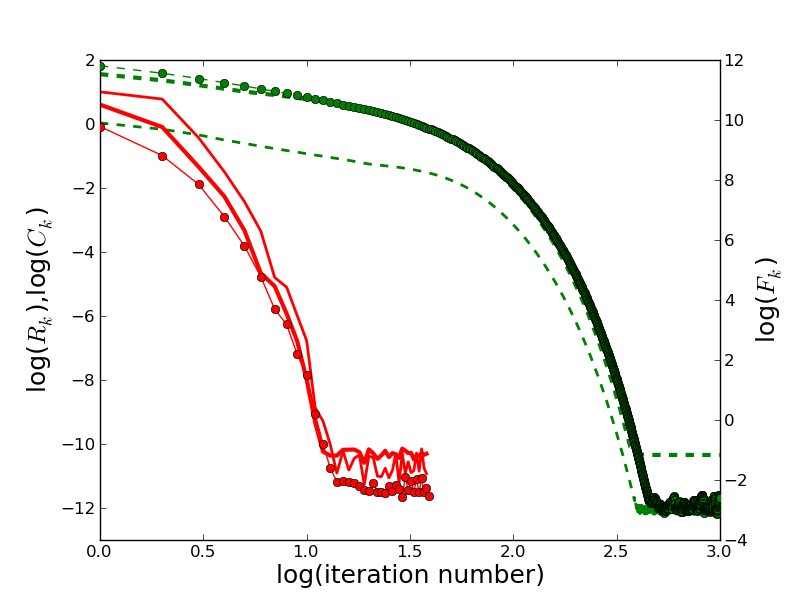
Figure 1: Typical relative error, $R_{k}$ (thin), convergence error, $C_{k}$ (thick) and $F_{k}$ (dotted) respectively for MALI (dash) and Broyden (full) vs. the number of iteration, for both scheme.

2.1 Broyden’s algorithm

The system of Eqs. (1) and (4) can be reformulated by defining a function $F$ acting on the set of $n^{(\tau)}=(n_{1}^{(\tau)},...,n_{i}^{(\tau)},...,n_{N_{L}}^{(\tau)})$ where $\tau$ is a discrete depth along the opacity scale used to sample our slab or atmosphere. $F$ is defined such as:

F_i^(τ)= ∑_j¡i [n_i^(τ)A_ij-(n_j^(τ)B_ji-n_i^(τ)B_ij)¯J_ij] (5)

$$-\sum\limits_{j>i} [n_{j}^{(\tau)}A_{ji}-(n_{i}^{(\tau)}B_{ij}-n_{j}^{(\tau)}B_{ji})\bar{J}_{ij}]$$

$$+\sum\limits_{j\neq i} (n_{i}^{(\tau)}C_{ij}-n_{j}^{(\tau)}C_{ji})$$

for $i\neq N_{\rm L}$ and, if $i=N_{\rm L}$

$$F_{i}^{(\tau)}=\sum\limits_{j=1}^{N_{L}}n_{j}^{(\tau)}-n_{t}\,.$$ (6)

Computations of $F$ requires repeated evaluations of scattering integrals $\bar{J}_{ij}$ – Eq. (2) – that we perform here using the well-know short-characteristics method with monotonic parabolic interpolation introduced by Auer & Paletou (1994).

In that frame, and using the Sherman-Morrison formula (see e.g., Press et al. 1992) which provides an analytical formula for the direct computation of the inverse of the Broyden matrix, our algorithm consists in the following steps. We choose an initial vector $n_{0}$, at every $\tau$ depth, and an initial Broyden matrix $B_{0}$; then we compute $B_{0}^{-1}$. The iterative scheme is such that:

$$\delta n_{k}=-B_{k}^{-1}F(n_{k})\,,$$ (7)

then update

$$n_{(k+1)}=n_{k}+\delta n_{k}\,,$$ (8)

then compute

$$\delta F_{k}=F(n_{(k+1)})-F(n_{k})\,,$$ (9)

and finally, update

$$B_{(k+1)}^{-1}=B_{k}^{-1}+\frac{(\delta n_{k}-B_{k}^{-1}\delta F_{k})\delta n_{k}^{T}B_{k}^{-1}}{(\delta n_{k}^{T}B_{k}^{-1})\delta F_{k}}$$ (10)

while ${\|F\|_{2}}>\varepsilon$. Practically, we have chosen $\varepsilon=10^{-2}$, which guarantees that we have reached a fully converged state (see also Fig. 1).

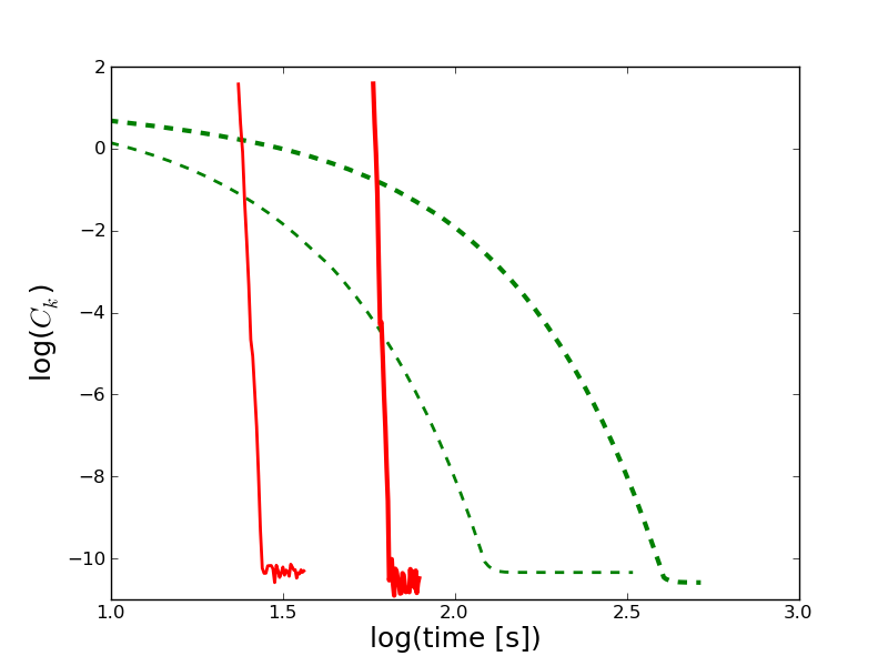
Figure 2: The convergence error, $C_{k}$, for MALI (dashed) and Broyden (full) are displayed vs. computing time for a 5-level H atom and, respectively, 5 (thin) and 8 (thick) points per decade in optical depth.

2.2 Initialization

The proper initialization of the Broyden scheme is a critical issue. We employed the following method which was tested as suitable, both from the standpoint of an adequate start and from the one of an acceptable computing time.

Before starting the iterative scheme, we assume LTE populations for our model-atom. In such a way, the grand function $F$ defined by Eqs. (5) and (6) can be fully evaluated. Then, we compute an initial Jacobian, $B_{0}$, using the finite difference scheme fdjac described by Press et al. (1992).

In the following figures relative to the timing properties of Broyden’s method vs. MALI, we shall always include the specific time necessary for the evaluation of $B_{0}$.

3 Comparison of Broyden vs. MALI

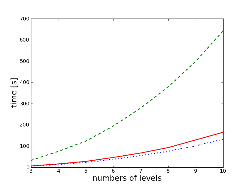
Figure 3: Respective computing times vs. number of levels of the H-atom model, for for MALI (dashed) and Broyden (full). The dash-dotted curve corresponds to the time required for the evaluation of the initial Jacobian.

We adopted the popular “flavor” of the MALI method, using a diagonal approximate operator, as described by Rybicki & Hummer (1991), and without acceleration of convergence schemes.

In order to compare the properties of the Broyden scheme vs. MALI, we adopted a 1D semi-infinite plane parallel slab model of $\tau_{\rm max}=10^{10}$, discretized in various number of points per decade in optical depth, using also 3 to 10 energy levels H-atom, inspired by the classic benchmark proposed by Avrett (1968; see also Léger & Paletou 2007). As in the latter, the slab temperature was fixed at 5000 K and the collisional rates set at $10^{5}\,{\mathrm{s}}^{-1}$. We also adopted the definitions initially proposed by Auer et al. (1994) for the relative error, from an iteration $(k)$ to another:

$$R_{k}={\left|\left|{{n_{(k)}-n_{(k-1)}}\over{n_{(k)}}}\right|\right|_{\infty}}\,,$$ (11)

and for the “convergence error”:

$$C_{k}={\left|\left|{{n_{(k)}-n_{(\infty)}}\over{n_{(\infty)}}}\right|\right|_{\infty}}\,,$$ (12)

where $n_{(\infty)}$ is the “fully converged” solution obtained, for a given method and model, after a large number of iterations. We also introduce the quantity

$$F_{k}={\|F_{(k)}\|_{2}}$$ (13)

i.e., the Euclidian norm of $F$, the function defined by Eqs. (5) and (6). Note that $F_{k}^{(M)}$ for the MALI method is defined by a modified Eq. (5) following the preconditioning strategy proposed by Rybicky & Hummer (1991).

3.1 Convergence

In Fig. 1, we display the rates of convergence of the Broyden and MALI methods, respectively. The convergence error $C_{k}$ for each method have been computed using population densities obtained once $F_{k}<{10}^{-2}$ in both cases. The case used here is a 5-level H atom with a 1D slab discretized by a 5 points per decade grid in optical depth. It is worth noting that, in order to reach $F_{k}<{10}^{-2}$ and a well-converged solution though, one should iterate up to reaching $R_{k}$ values as small as ${10}^{-10}$ typically. In terms of number of iterations, Broyden typically beats MALI of more than one order of magnitude. However, the quite distinct nature of each method makes such a comparison incomplete. Hereafter, we carry on such an analysis but we shall compare respective computing times.

3.2 Sensitivity to the spatial (optical depth) refinement

In Fig. 2, we turn to an analysis of the respective timing properties of Broyden and MALI. It is shown that Broyden, again, always beats MALI by a typical factor of the order of about 4-5 in time. It is also the case when the spatial grid refinement is increased from 5 to 8 points per decade, for instance. It is important to note that timings given for Broyden include the computation of the initial matrix $B_{0}$. This is why the rates of convergence displayed for the Broyden method do not start at $t=0$ in Fig. 2.

3.3 Sensitivity to the number of transitions

A next important point to investigate relates to the advantage of Broyden against MALI when an increasing number of atomic transitions is considered. Again, as demonstrated in Fig. 3, the full Broyden iterative process is always significantly faster than MALI. In general, the gain due to the Broyden method is of the order of 4-5 in total computing time. This is less than the the gain of the order of 8 already reported by Koesterke et al. (1992), although their method of reference was presumably different from MALI.

3.4 Discussion

We are aware that the MALI method can be speeded-up by acceleration of convergence schemes (see e.g., Auer 1991). However the most significant improvements in the field of iterative methods for the non-LTE radiative transfer problem were brought by the introduction of the Gauss-Seidel (GS) and Successive Over-Relaxation (SOR) methods (Trujillo Bueno & Fabiani Bendicho 1995). It was already shown, for instance, that SOR always beats both Jacobi (i.e., accelerated $\Lambda$-iteration with the diagonal of the full $\Lambda$ operator as an approximate operator) and GS, even when Ng acceleration of convergence is applied.

Beyond the fact that Broyden is significantly faster than MALI, we can also add that Broyden is as competitive as the SOR method, according to Paletou & Léger (2007; see their Table 1 where comparable timing and the corresponding iteration numbers were given for MALI, as we used it in the present study, GS and SOR).

The Broyden method is also potentially more advantageous than MALI and GS/SOR, because of its intrinsic capability to deal with the self-consistent evaluation of the electron density in a multilevel non-LTE problem, if necessary – a problem for which MALI needs to plug-in a Newton-Raphson scheme to it, as proposed by Heinzel (1995) and Paletou (1995).

Another important point is that, as indicated in our Fig. 3, a great deal of time of our Broyden code is spent in the computation of the initial Jacobian, a task which can be performed with great advantage using parallel computing. The inner structure of the fdjac routine permits, indeed, parallelization with a high scalability.

As a final comment, it is also important to consider that Broyden’s method can be easily implemented in already existing codes, without the need of modifying the formal solver, unlike with GS/SOR methods.

4 Conclusion

We propose an alternative method for the solution of the non–LTE multilevel radiation transfer problem. It is based on Broyden’s method for the solution of nonlinear systems of equations. The method is easy to implement and it is about of factor of 4.5 times faster than the well-known MALI method. Another advantage is that it does not require any modification of usual formal solvers, as it is the case for GS-SOR methods developed after MALI. It is also potentially very well-suited for parallel computing. Further tests will include the self-consistent treatment of the ionization balance, usually treated together with MALI with a Newton-Raphson scheme. In a next step, we shall consider more demanding models such as H₂O, for instance.

References

- (1) Auer, L.H. 1991, in: Stellar Atmospheres: Beyond Classical Models, NATO ASI Series (Dordrecht: Reidel)
- (2) Auer, L.H. & Mihalas, D. 1969, ApJ, 158, 641
- (3) Auer, L.H. & Paletou, F. 1994, A&A, 285, 675
- (4) Auer, L.H., Fabiani Bendicho, P. & Trujillo Bueno, J. 1994, A&A, 292, 599
- (5) Broyden, C.G. 1965, Math. Comp., 19, 577
- (6) Elitzur, M. & Asensio Ramos, A. 2006, MNRAS, 365, 779
- (7) Heinzel, P. 1995, A&A, 299, 563
- (8) Koesterke, L., Hamman, W.-R.. & Kosmol, P. 1992, A&A, 255, 490
- (9) Mihalas, D. 1978, Stellar Atmospheres (San Francisco: Freeman)
- (10) Paletou, F. 1995, A&A, 302, 587
- (11) Paletou, F. & Léger, L. 2007, JQSRT, 103, 57
- (12) Press, W.H. et al. 1992, Numerical recipes (Cambridge: University Press)
- (13) Rybicki, G.B. & Hummer, D.G. 1991, A&A, 245, 171
- (14) Socas-Navarro, H. & Trujillo Bueno, J. 1997, ApJ, 490, 383
- (15) Trujillo Bueno, J., & Fabiani Bendicho, P. 1995, ApJ, 455, 646