Dynamics at and near conformal quantum critical points

Abstract

We explore the dynamical behavior at and near a special class of two-dimensional quantum critical points. Each is a conformal quantum critical point (CQCP), where in the scaling limit the equal-time correlators are those of a two-dimensional conformal field theory. The critical theories include the square-lattice quantum dimer model, the quantum Lifshitz theory, and a deformed toric code model. We show that under generic perturbation the latter flows toward the ordinary Lorentz-invariant (2+1) dimensional Ising critical point, illustrating that CQCPs are generically unstable. We exploit a correspondence between the classical and quantum dynamical behavior in such systems to perform an extensive numerical study of two lines of CQCPs in a quantum eight-vertex model, or equivalently, two coupled deformed toric codes. We find that the dynamical critical exponent $z$ remains 2 along the $U(1)$-symmetric quantum Lifshitz line, while it continuously varies along the line with only ${\mathbb{Z}}_{2}$ symmetry. This illustrates how two CQCPs can have very different dynamical properties, despite identical equal-time ground-state correlators. Our results equally apply to the dynamics of the corresponding purely classical models.

I Introduction

The study of critical properties of classical statistical mechanics systems with stochastic relaxational dynamics has a venerable history.HH More recently, a class of quantum systems closely related to classical systems with stochastic dynamics has come under intense study. Here, each basis element of the Hilbert space of the two-dimensional quantum system corresponds to a configuration in a two-dimensional classical system. This in itself is not unusual; what is special about this class is that the Hamiltonian is chosen so that the ground state is written in terms of the Boltzmann weights of the classical model. One significant consequence of this relation between quantum and classical models is that correlators in the ground state of such a Hamiltonian are the same as those of the classical model. This means that the phase diagrams of the quantum and classical models are closely related.

The quantum dimer model RK is an example of this class of quantum systems. On the square lattice, it is a canonical example of the conformal quantum critical points to be discussed in this paper, while on the triangular lattice is a canonical example of topological order.MS The Hilbert space is spanned by close-packed hard-core dimer configurations. The quantum ground state is the equal-amplitude sum over all such dimer configurations. A Hamiltonian having this ground state can easily be constructed by using a technique first developed in this context by Rokhsar and Kivelson RK (RK). It typically is a sum of local projection operators, each annihilating the ground state, and will be reviewed in Sec. II.2.

In particular, this provides a way to discover and analyze new quantum critical points in two spatial dimensions. Whenever a ground state in two dimensions has a correlator of local operators algebraically decaying with distance, all local Hamiltonians must be gapless.Hastings Thus if the ground state of an RK Hamiltonian is described by a critical classical theory, the quantum theory must be critical as well. Since well-understood quantum critical points in two dimensions are few and far between, such RK Hamiltonians are quite interesting.FootnoteFrustration

Indeed some of the best-understood quantum critical points in two dimensions were found by analyzing RK Hamiltonians. A great deal is known about critical points in rotationally invariant two-dimensional classical models, because these critical points are not only scale invariant, but conformally invariant as well. Two-dimensional conformal symmetry has an infinite number of generators, and so is very powerful. It can be used not only to identify many classes of critical points, but to explicitly compute correlation functions in the scaling limit, even when the systems are strongly interacting. Because the ground state correlators are those of the classical theory, these results can then be carried over to the quantum case. In fact, the ground state itself becomes conformally invariant in the scaling limit, as detailed in Ref. AFF, . For this reason, these theories were dubbed conformal quantum critical points.

The static behavior of conformal quantum critical points is well understood because of this connection to conformal field theory. Their dynamical behavior, however, is another story. Only in an exactly solvable case Henley97 ; AFF ; Senthil05 , dubbed the quantum Lifshitz theory, has the quantum dynamics has been studied in depth. Here the ground-state correlators can be written in terms of classical correlators of a free massless scalar field. Moreover, the quantum Hamiltonian remains quadratic (although not Lorentz-invariant), and so everything in principle can be computed.Senthil05

One purpose of this paper is to study the dynamics of more complex conformal quantum critical points. A key example, which we will study in detail, are the two lines of conformal quantum critical points in the quantum eight-vertex model of Ref. AFF, . The first of these two lines exhibits an additional $U(1)$ symmetry, which reduces the quantum eight-vertex model to a quantum six-vertex model whose scaling limit corresponds precisely to the quantum Lifshitz model mentioned above. So, while the quantum six-vertex model is not exactly solvable, the field theory describing its scaling limit is. There is, however, an RK Hamiltonian whose ground state is that of the classical six-vertex model. The second critical line corresponds to the full quantum eight-vertex model. This line is not exactly solvable on the lattice or in the scaling limit, although again the ground state of an RK Hamiltonian can be found explicitly. The equal-time correlators on the two critical lines can be mapped onto each other, because the two corresponding classical theories are dual to each other.Baxbook

In general, different dynamical symmetry classes are possible for a given static universality class, depending, e.g., on whether the dynamics possesses conservation laws or not.HH We find here that despite the identical equal-time correlators, the dynamical behavior of the two critical lines is indeed quite different. In the quantum Lifshitz theory, the dynamical critical exponent remains $z=2$ all along the line, while along the other line, this exponent is found to vary. In the language of Ref. HH, , the latter possesses Model A dynamics, i.e.  the dynamics has no conservation law, and only Ising ${\mathbb{Z}}_{2}$ symmetry. In the former, however, the dynamics respects a $U(1)$ symmetry, and so has a conserved quantity; this corresponds to Model B. Both theories possess an exactly marginal operator, and the exponents of the equal-time correlators vary continuously along the critical lines. However, we note that the presence of an exactly marginal operator implies the existence of a $U(1)$ symmetry only in two classical dimensions, not in a full two-dimensional quantum theory.

To do this analysis, we exploit the fact that the connection between the classical and quantum models goes deeper than the equal-time correlators. As described in refs. Henley97, ; Henley04, ; Castelnovo05, , much can be learned about the quantum dynamics by studying the classical ones. This means in particular that in some cases the dynamical critical exponent $z$ in the quantum model can be found by doing classical Monte Carlo simulations. Since one point along the $z\neq 2$ line amounts to doing classical Ising dynamics, we make contact with decades of numerical studies LandauBinder here.

Even though an RK Hamiltonian is fine-tuned, when it describes a phase with topological order, this physics persists under (at least small) deformations. This has been demonstrated numerically in several examples,MS ; Trebst07 ; Vidal09 ; Tupitsyn10 ; Vidal10 and recently been derived rigorously. Klich ; Bravyi10 The robustness of topological order near RK points is not surprising, given that the phase is gapped. The argument of course does not apply at conformal quantum critical points, and there is no reason to expect that these will remain critical under generic perturbations. Even though the square-lattice quantum dimer model is critical with seemingly no fine tuning, this is a consequence of the highly constrained behavior of dimer models. In a more general setting, it has been shown that this quantum critical point typically has several relevant perturbations, as well as a host of dangerously irrelevant operators.Fradkin03 ; Balents03

Thus an interesting question is if a conformal quantum critical point is isolated, or if it is part of a phase boundary. In renormalization group language, the question is whether a relevant perturbation causes a flow to another quantum critical point, or into a gapped phase. We will present substantial evidence that the Ising conformal quantum critical point is continuously connected to the usual 2+1d Ising critical point.

The outline of the remainder of the paper is as follows. In Sec. II we review some well known models with RK Hamiltonians, the quantum Lifshitz theory and the quantum dimer model. We also display a general connection between classical dynamics and quantum dynamics in theories with RK Hamiltonians. In Sec. III, we discuss the dynamics of the Ising conformal quantum critical point in two spatial dimensions, i.e. the quantum critical point whose ground state is written in terms of the Boltzmann weights of the critical classical 2d Ising model. RK Hamiltonians are strongly fine-tuned, and so we show in Sec. IV that generic perturbations of the lattice model generate a crossover from the $d=2$ dimensional dynamics with dynamical critical exponent $z\approx 2.167$ (and 2D static correlation length exponent $\nu=1$), to the critical dynamics of the (2+1)-dimensional classical Ising universality class with $z=1$ (and $\nu\approx 0.632$). In Sec. V we discuss the case of the dynamics of two coupled copies of the deformed toric code, or in the equivalent classical case, two coupled copies of the critical Ising model. There are two critical lines, whose equal-time correlators can be mapped into each other’s by two-dimensional classical duality. We show that these lines correspond to different dynamic universality classes. In the case without $U(1)$ symmetry, we will present numerical results that indicate that along with the static critical exponents, the dynamical critical exponent $z$ also varies with the couplings.

II Conformal quantum critical points and RK Hamiltonians

The great progress made in understanding conformal quantum points came from considering specific ground state wavefunctions. Once a particular ground state is specified, it is usually (but not always) straightforward to find some RK Hamiltonian with this ground state.

All the models we study have Hilbert spaces whose basis elements are labeled by configurations in some classical two-dimensional model. Let ${\cal C}$ label a classical configuration, and $w({\cal C})$ be its Boltzmann weight. Then let $|{\cal C}\rangle$ be the corresponding basis element of the quantum Hilbert space. Here we take the simplest choice for the inner product, the orthonormal one. In a lattice model with discrete degrees of freedom,

$$\langle{\cal C}^{\prime}|{\cal C}\rangle=\delta_{CC^{\prime}}\ .$$ (1)

With continuous degrees of freedom as in a field theory, the Kronecker delta is replaced by a Dirac delta function.

To find a conformal quantum critical point (CQCP) by this method, the classical model must be critical and isotropic, and the Boltzmann weights $w({\cal C})$ must be real and non-negative for all ${\cal C}$. Then the (unnormalized) ground state wave function

$$|\Psi\rangle=\sum_{\cal C}\sqrt{w({\cal C})}|{\cal C}\rangle$$ (2)

is that of a CQCP. The expectation value of any diagonal operator ${\cal D}$ in the ground state is identical to that found in the classical theory:

$$\frac{\langle\Psi|{\cal D}|\Psi\rangle}{\langle\Psi|\Psi\rangle}=\frac{\sum_{\cal C}w({\cal C}){\cal D}({\cal C})}{\sum_{\cal C}w({\cal C})}\ ,$$

where ${\cal D}({\cal C})\equiv\langle{\cal C}|{\cal D}|{\cal C}\rangle$ is by definition the value of ${\cal D}$ in configuration ${\cal C}$.

At first glance, it appears that for any local dynamics possible in a critical classical system, there exists a corresponding conformal quantum critical point. This is not true, because in a quantum theory one of course weights by the absolute value of the amplitude squared. Some classical Euclidean field theories like the Wess-Zumino-Witten models are only critical when the action includes an imaginary term. Thus even if one has an RK Hamiltonian whose ground state includes such a term, this term disappears from $|\Psi|^{2}$, and so the correlators will not decay algebraically.AFF

II.1 The quantum Lifshitz theory

An important example of a CQCP is given by the quantum Lifshitz theory. This is an exactly solvable field theory that describes, among other things, the scaling limit of the square-lattice quantum dimer model. Here the degrees of freedom are given by a scalar field $\varphi(x)$, which is a smooth map of all points $x$ on some two-dimensional manifold to a circle. The Boltzmann weight of the classical model for a given field configuration is simply $w=e^{-S_{2d}}$, where $S_{2d}$ is the standard action for a free massless scalar field:

$$S_{2d}(\varphi)=\kappa\int d^{2}x(\nabla\varphi)^{2}\ ,$$ (3)

with $\kappa$ an arbitrary parameter. As discussed in Ref. AFF, , this weight defines a ground-state wave functional, such that all diagonal correlators in the quantum model are those of a classical massless scalar field in two dimensions.

The action $S_{2d}$ is invariant under conformal transformations of $x$, so the Boltzmann weights for the quantum Lifshitz ground state are invariant as well. It also possesses an additional symmetry, under shifts (constant in space) of $\varphi$. This $U(1)$ symmetry is also a symmetry of the quantum Lifshitz Hamiltonian

$$H_{QL}=\frac{1}{2}\int d^{2}x\left[\Pi^{2}+\kappa^{2}(\nabla^{2}\varphi)^{2}\right]\ ,$$ (4)

where the canonical conjugate field $\Pi(x)$ obeys $[\Pi(x),\varphi(x^{\prime})]=i\delta^{(2)}(x-x^{\prime})$. For the examples of interest here, the field $\varphi$ is periodic, i.e. $\varphi=\varphi+2\pi$. The resulting vortex operators, however, are irrelevant at a CQCP.AFF

This Hamiltonian is not a sum of projection operators like the RK lattice Hamiltonian is. However, it is very similar: it can be written AFF as the integral over local terms of the form $Q^{\dagger}(x)Q(x)$. Such a Hamiltonian necessarily has non-negative eigenvalues, and so any state annihilated by $Q(x)$ for all $x$ is a zero-energy ground state. The ground state (2) with $w=e^{-S_{2d}}$ is indeed annihilated by all $Q(x)$.

Since the quantum Lifshitz Hamiltonian is quadratic in the fields, it is exactly solvable, and so much more than just the ground-state correlators can be computed.Senthil05 In particular, by writing down the three-dimensional Euclidean action for this theory

$$S_{3d}=\frac{1}{2}\int d^{2}xdt\left[\left(\frac{\partial\varphi}{\partial t}\right)^{2}+\kappa^{2}(\nabla^{2}\varphi)^{2}\right]\ ,$$ (5)

one sees immediately that the dispersion relation is $E\propto k^{2}$, and so the dynamical critical exponent is $z=2$. As we will discuss below, we believe that a generic $U(1)$-invariant CQCP has $z=2$.

II.2 Quantum dimers on the square lattice

The square-lattice quantum dimer model is an example of a lattice model with a conformal quantum critical point.RK Each basis element ${\cal C}$ corresponds to a configuration of dimers stretching between neighboring sites on the square lattice. The weight $w({\cal C})=1$ for all configurations that have exactly one dimer touching each site, and is zero for all configurations violating the constraint. It has long been known that correlators in the classical dimer model on the square lattice are algebraically decaying.FS Thus by Hastings’ theorem,Hastings the square-lattice quantum dimer model is critical.

The RK Hamiltonian here was described in the original paper by Rokhsar and Kivelson.RK It is a sum of local projection operators with the ground state annihilated by each projector individually. Each term acts non-trivially on a single plaquette, projecting each of the two configurations with two dimers on this plaquette onto their difference. It annihilates all other configurations on that plaquette. Each such projector indeed annihilates the equal-amplitude sum over all configurations.

An elegant argument Henley97 indicates that the scaling limit of the square-lattice quantum dimer model is $\kappa^{-1}=2\pi$ of the quantum Lifshitz model: First, one identifies the classical model as having the free scalar field action $S_{2d}$ in (3) with $\kappa^{-1}=2\pi$. This follows from a Coulomb-gas mapping, done here by rewriting the dimer degrees of freedom in terms of a classical “height”, an integer-value degree of freedom on every site of the lattice. It is then natural to assume that the height becomes the continuous field $\varphi$ in the scaling limit. The value $\kappa$ is then identified by comparing the scaling dimensions determined from the exact computation to those in the classical 2d scalar field theory. The ground state in the scaling limit therefore must be of the form (2), because all its diagonal correlators are the same as those of $S_{2d}$. The Hamiltonian (4) by construction annihilates this. Moreover, note that the quantum dimer model has a $U(1)$ symmetry. The Hamiltonian preserves both the overall number of dimers and their “winding number” of dimers. (The winding number is defined by $\sum_{j}n_{j}(-1)^{j}$, where $j$ labels the links around a cycle and $n_{j}=1$ for occupied links and $n_{j}=0$ for unoccupied.) This requires that only derivatives of $\varphi$ can appear in the Hamiltonian, which indeed is a property of (4).

Figure 1: The finite-size gap of the quantum dimer model as a function of the system size. The gap scales as $\Delta\propto L^{-2.01(2)}$ indicating that $z=2.01(2)$.

Finding the dynamical scaling exponent $z$ provides another check that the scaling limit of the square-lattice quantum dimer model is given by the quantum Lifshitz theory. The quantum dimer model is not solvable, even though its ground state is known exactly. We thus need to find $z$ numerically; we do this by studying the finite-size scaling of the gap. Our method is described in Appendix A. We find that $z=2.01(2)$, as shown in Fig. 1. This is in excellent agreement with the exact value $z=2$ for the quantum Lifshitz theory, as seen from (5), and previous numerical results.Laeuchli08 As such it also provides a nice consistency check on our numerical method.

II.3 RK Hamiltonians from classical stochastic dynamics

For classical systems with (positive) Boltzmann weights $w({\cal C})$, every relaxational stochastic dynamics is knownHenley04 to give rise to a “RK Hamiltonian”: time-dependent probabilities $p_{\cal C}(\tau)\geq 0$, satisfying a “master equation”. The master equation is written in terms of a “transition matrix” $W_{{\cal C},{\cal C}^{\prime}}$, where for different configurations ${\cal C}\not=$ ${\cal C}^{\prime}$, the matrix element $W_{{\cal C},{\cal C}^{\prime}}\geq 0$ denotes the transition rate from ${\cal C}^{\prime}$ to ${\cal C}$. The diagonal element defined by $W_{{\cal C},{\cal C}}:=$ $-\sum_{{\cal C}^{\prime}\not={\cal C}}W_{{\cal C}^{\prime},{\cal C}}$ denotes the transition rate out of state ${\cal C}$. The master equation is then

$$\frac{d}{d\tau}p_{\cal C}(\tau)=\sum_{{\cal C}^{\prime}}\ W_{{\cal C},{\cal C}^{\prime}}\ p_{{\cal C}^{\prime}}(\tau)\ .$$ (6)

The probabilities relax at long times to the classical equilibrium distribution

$$p_{\cal C}(\tau)\ \to w({\cal C})$$ (7)

when detailed balance

$$w({\cal C})\ W_{{\cal C}^{\prime},{\cal C}}\ =\ W_{{\cal C},{\cal C}^{\prime}}\ w({\cal C}^{\prime})$$ (8)

is satisfied.

A slight re-writing of the master equation (6) gives a generalization of the RK Hamiltonian. The rescaled transition matrix

$${\widetilde{W}}_{{\cal C},{\cal C}^{\prime}}\ \equiv\frac{1}{\sqrt{w({\cal C})}}\ W_{{\cal C},{\cal C}^{\prime}}\ \sqrt{w({\cal C}^{\prime})}\ ,$$ (9)

is (real) symmetric due to detailed balance Eq. (8). Letting ${\tilde{p}}_{\cal C}(\tau)\equiv p_{\cal C}(\tau)/\sqrt{w({\cal C})}$, the rewritten master equation is

$$\frac{d}{d\tau}{\tilde{p}}_{\cal C}(\tau)=\sum_{{\cal C}^{\prime}}\ {\widetilde{W}}_{{\cal C},{\cal C}^{\prime}}\ {\tilde{p}}_{{\cal C}^{\prime}}(\tau)\\$$ (10)

This is a Schrödinger equation in imaginary time $\tau$ with Hamiltonian ${H}_{{\cal C},{\cal C}^{\prime}}=(-1){\widetilde{W}}_{{\cal C},{\cal C}^{\prime}}$ for the time-dependent quantum state

$$|\Psi(t)\rangle=\sum_{\cal C}\ {\tilde{p}}_{\cal C}(t)\ |{\cal C}\rangle,$$ (11)

Note that ${\widetilde{W}}_{{\cal C},{\cal C}^{\prime}}$ and ${W}_{{\cal C},{\cal C}^{\prime}}$ are related by a similarity transformation and so have the same spectrum. The Hamiltonian thus has the same spectrum as that of the relaxational dynamics, Eq. (6). The state (11) relaxes, due to Eq. (7), at long imaginary times $\tau$ to the ground state Eq. (2). Thus this construction indeed provides a generalization of the RK-type Hamiltonian and ground state.

In the present formulation, ${\cal C}$ denotes configurations of classical variables on a lattice. When the system with classical Boltzmann weights $w({\cal C})$ possesses an equilibrium critical point, a universal continuum field theory description emerges upon coarse graining for both the static as well as for the dynamic correlations. The resulting dynamic universality classes are classified within the well known framework of Hohenberg and Halperin. HH For example, the Ising conformal quantum critical point discussed below in section III is described by the Model A dynamical universality class of Hohenberg and HalperinHH (describing dynamics lacking any conservation law). The quantum Lifshitz universality class, however, possesses a $U(1)$ symmetry, so that this belongs to the Model B universality class.

The classical dynamics are conventionally described by a time-dependent Landau-Ginzburg equation with stochastic Langevin-type noise, or equivalently, as a Fokker-Planck equation for the time-evolution of the probability distribution for the coarse-grained classical degrees of freedom. It is well knownZinnJ that if one performs the corresponding similarity transformation to make the linear operator appearing in the Fokker-Planck equation Hermitian, the Fokker-Planck equation turns into the coarse-grained analog of the Schrödinger equation, Eq. (10), in imaginary time. Specifically, for a classical statistical mechanics system in $d$ spatial dimensions described, e.g., by a static (real) Landau-Ginzburg action $S{\{\phi_{a}(x)\}}$ for coarse-grained classical degrees of freedom $\{\phi_{a}(x)\}$, the resulting quantum Hamiltonian is again of the form

$$H=\frac{1}{2}\int d^{d}x\ Q_{a}^{\dagger}(x)Q_{a}(x)$$ (12)

generalizing Eq.  (4), where

$$Q_{a}(x) = \frac{1}{\sqrt{2}}\left(\frac{\delta}{\delta\phi_{a}(x)}+\frac{1}{2}\frac{\delta S}{\delta\phi_{a}(x)}\right)$$

$$Q^{\dagger}_{a}(x) = \frac{1}{\sqrt{2}}\left(-\frac{\delta}{\delta\phi_{a}(x)}+\frac{1}{2}\frac{\delta S}{\delta\phi_{a}(x)}\right)$$ (13)

This implies very generally that the ground state wave function $\Psi(\{\phi_{a}(x)\})=$ $(1/\sqrt{Z})\exp\{-\frac{1}{2}S{\{\phi_{a}(x)\}}\}$ is given by the classical Boltzmann weight ($Z$ denotes the classical partition function). Thus the (in general non-Hermitian) linear operator appearing in the Fokker-Planck equation becomes, after similarity transform, the negative of the (Hermitian) quantum Hamiltonian, $(-1)H$. All its eigenfunctions are positive.

The Hamiltonians of the form of Eq.  (12) are clearly very special. One may ask if there exists a symmetry principle which constrains Hamiltonians to be fine-tuned to this very particular form. Indeed, there exists such a symmetry. It is again well knownZinnJ that classical relaxational stochastic dynamics can be viewed as being invariant under certain supersymmetry transformation.DijkgraafOrlandoReffert The property that equal-time correlation functions converge at large times to static equilibrium correlation function can then be seen as a direct consequence of the underlying supersymmetry. The perturbation of the Ising conformal quantum critical point discussed in Sec. IV can thus be viewed as breaking the supersymmetry.

This procedure makes obvious the relation between classical dynamics and RK Hamiltonians. In fact, the generic way of constructing RK Hamiltonians in field theory discussed in Ref. AFF, is formally identical to that in Eqs. (12) and (13). For example, the quantum Lifshitz Hamiltonian (4) arises with one field $\varphi$ and setting $S=S_{2d}$ from Eq. (3).Henley97 ; AFF

III Quantum and classical dynamics in the Ising model

The Hilbert spaces of the lattice models we consider for the remainder of the paper are simply those of the Ising model on the square lattice. Namely, at every site we have a spin (i.e. a two-state quantum system), and all the Hamiltonians we consider are invariant under flipping all the spins. We write the Hamiltonians in terms of the Pauli matrices $\tau^{a}_{\alpha}$ acting on the spin at site $\alpha$.

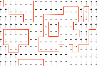
Figure 2: Sketch of a typical domain wall configuration separating regions of opposite spins.

For both pedagogical and physical reasons, it is often convenient to describe the Hilbert space in terms of domain walls instead of spins. There is a two-to-one mapping from spin configurations to domain walls obtained simply by drawing a lines on the links of the dual lattice separating regions of different spins. A typical configuration is illustrated in Fig. 2. Each domain wall is a two-state system, so we define the Pauli matrices $\sigma^{a}_{k}$ acting on the link $k$ analogously to the spins. However, the domain walls cannot end or branch, so there must be an even number of domain walls at each site. In an equation, we constrain

$$\prod_{k\hbox{ touching }\widehat{\alpha}}\sigma^{z}_{k}=1\ ,$$ (14)

for all sites $\widehat{\alpha}$ on the dual lattice. For the obvious reason, these domain walls are often referred to as “loops”.

III.1 The toric-code ground state

Let us first consider an important non-critical case, closely related to the mother of all lattice models for topological quantum computation, the toric code.Kitaev97 Here the ground state (2) is a sum over all Ising configurations with the same amplitude $\sqrt{w({\cal C})}=1$. Thus the associated classical model is simply the Ising model at infinite temperature. Equivalently, the ground state can be viewed as a sum over all loop configurations with equal amplitude. Correlators of local objects in the ground state (e.g. whether a link is occupied by a loop or not) are obviously finite-range.

The gapped RK Hamiltonian having this ground state is simply the sum over all possible single-spin flips:

$$H_{T=\infty}=\sum_{\alpha}(1-\tau^{x}_{\alpha})\ .$$ (15)

In terms of domain walls/loops, this acts on the four links on the dual lattice surrounding each site $j$, removing a wall when there is one and adding a wall when there isn’t:

$$\tau^{x}_{\alpha}=\prod_{p\in\square_{\alpha}}\sigma^{x}_{p}$$ (16)

where the product is over the four links on the plaquette on the dual lattice surrounding the site $\alpha$.

This equal-amplitude sum over all loops/domain walls is the same ground state as in the toric code. The difference between the models is that in the toric code, the constraint (14) is not imposed. Rather, a diagonal term is added to the Hamiltonian to give an energy for every sites with an odd number of domain walls touching it. The energy penalty then precludes any configuration with an odd number of domain walls at a site from appearing in the ground state.

Since each term in the Hamiltonian (15) commutes with each of the others, this model is trivially solvable, and the sum over all loops is indeed the ground state. On the disk, this ground state is unique. On the torus, there are four ground states, corresponding to the choices of having zero or one loops go around each cycle. It is easy to see that the model is gapped; excited states correspond to having plaquettes with the eigenvalue $-1$ of $\tau^{x}$. This ground state has topological order, and so has been the subject of intense study in recent years.

III.2 The Ising CQCP

Thinking about the toric code in terms of Ising spins makes it clear how to find a conformal quantum critical point separating the phase with topological order from an ordered phase. We simply need to change the weight in the ground state to correspond to that in the classical two-dimensional Ising model at non-infinite temperature. In loop language, this corresponds to adding a weight per unit length $2\eta$, so that

$$w({\cal L})=\eta^{2n_{\cal L}}$$

where $n_{\cal L}$ is the number of links covered by loop. In the quantum theory, we can write

$$\left(\sum_{k=1}^{N}\sigma^{z}_{k}\right)|{\cal L}\rangle=(2n_{\cal L}-N)|{\cal L}\rangle$$

for $N$ links. The ground state is then simply

$$|\Psi\rangle=\sum_{\mathcal{L}}\eta^{n(\mathcal{L})}|\mathcal{L}\rangle\ .$$ (17)

An RK Hamiltonian with the ground state (17) for general $\eta$ can be found by including a potential that weights links. We will show below that the Hamiltonian found in Ref. AFF, gives two copies; a simpler-to-write form is CC

$$H_{Ising}=\sum_{\alpha}\left(\prod_{p\in\square_{\alpha}}\eta^{\sigma^{z}_{p}}-\prod_{p\in\square_{\alpha}}\sigma^{x}_{p}\right)\ .$$ (18)

This Hamiltonian can be written as a sum over projectors, each projector breaking into two-by-two blocks. Note that there is no manifest $U(1)$ symmetry like there is in the quantum dimer model.

The 2d Ising critical point is at $\eta=\eta_{c}$, where

$$\eta_{c}=(1+\sqrt{2})^{-1/2}$$ (19)

Any local Hamiltonian such as (18) having (17) with $\eta=\eta_{c}$ as a ground state must be quantum critical by Hastings’ theorem. We call the Hamiltonian (18) with $\eta=\eta_{c}$ the Ising CQCP.

This quantum Hamiltonian imposes a dynamics on the spins identical to the usual classical dynamics with local updates. Thus the dynamical exponent $z$ is the same in two cases. There have been numerical determinations of $z$ for decades; the current value from Ref. Nightingale, is $z=2.1667(5)$. This is slightly larger than the $z=2$ value for the quantum dimer model and the quantum Lifshitz theory; below in Sec. V we explain how to adapt an argument of Ref. AFF, to suggest that $z\geq 2$ for CQCPs. For the Ising case here, a rigorous inequality requires that $z\geq 7/4$.Halperin73

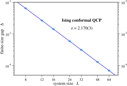
Figure 3: The finite-size gap of Hamiltonian (18) at the Ising CQCP $\eta_{c}$ as a function of the system size. The gap scales as $\Delta\propto L^{-2.170(3)}$ indicating that $z=2.170(3)$.

We have rechecked this number using our numerical methods described in Appendix A, and find the same result, see Fig. 3. We note that one needs to simulate the classical Ising model with the Monte Carlo transition matrix that is proportional to the quantum Hamiltonian. In this case, the transition matrix has the following form

$$W_{{\cal C},{\cal C}^{\prime}}=\eta^{4}\sqrt{\frac{w({\cal C}^{\prime})}{w({\cal C})}},$$

where $w({\cal C})$ and $w({\cal C^{\prime}})$ are the weights of the configurations before and after update (single spin flip). This transition matrix leads to the same dynamical exponent as the Metropolis transition matrix.

IV Flow from 2D Ising to 3D Ising

Another interesting way to deform the toric code is to include the more conventional Ising nearest-neighbor interaction. In this section, we study the phase diagram of the toric code deformed by this interaction and the special RK-type interaction in (18). We will show that including this term causes a flow from the Ising CQCP with 2d Ising critical exponents to the usual $z=1$ Ising critical transition in $2+1$ dimensions.

Adding the Ising nearest-neighbor interaction deforms Eq. (18) to

$$H=-\frac{1}{\eta^{4}}\sum_{\alpha}\left[\tau_{\alpha}^{x}+\frac{1}{\eta^{4}}\prod_{\beta}\eta^{\tau_{\alpha}^{z}\tau_{\beta}^{z}}-\frac{h\eta^{4}}{2}\sum_{\beta}\tau_{\alpha}^{z}\tau_{\beta}^{z}\right],$$ (20)

where the sites $\beta$ are the nearest neighbors of $\alpha$. We include a factor of $1/\eta^{4}$ compared to Eq. 18 for convenience. In terms of the link degrees of freedom, the extra term is simply a loop tension $-h\sum_{p}\sigma^{z}_{p}$. The other diagonal term in $H$ can also be thought of as a loop tension, but fine-tuned to make the ground state have the weighting of the 2d classical Ising model.

The Hamiltonian (20) reduces to that of the 2D transverse field Ising model on the square lattice for $\eta=1$. There is a phase transition at $h\approx 0.32847$,blote which is in the 3D Ising universality class with the dynamical critical exponent $z=1$ and the correlation length exponent $\nu\approx 0.632$. From the discussion in the previous section, we know that there is a conformal critical point at $h=0$ and $\eta=\eta_{c}$. This phase transition is in the 2D Ising universality class with the dynamical critical exponent $z\approx 2.167$ and the correlation length exponent $\nu=1$.

IV.1 Phase diagram

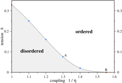
Figure 4: Phase diagram in the $h$-$1/\eta$ plane. Error bars are smaller than the symbol size. The line guides the eye. The whole transition line has $z=1$ except for one point at $h=0$ and $1/\eta=(1+\sqrt{2})^{1/2}$. For the two points indicated as A and B, we extract the critical exponent $\nu$ from data collapses of the Binder cumulants in Figs. 5 and 7, respectively.

The interesting question is if these two critical points are connected by a line of phase transitions, or describe disconnected regions in parameter space. We find convincing numerical evidence that the former is true. The full phase diagram in the $h-1/\eta$ plane is shown in Fig. 4. The CQCP at $h=0$ and $\eta=\eta_{c}$ is unstable under perturbations by both $h$ and $\eta$. Along a particular line in this plane, there is a flow from the Ising CQCP to the 2+1d Ising fixed point. The whole phase boundary in Fig. 4 has 3D Ising exponents except for one point.

This phase diagram was mapped out by using a variant of the continuous-time quantum Monte Carlo algorithm.rieger We measure the Binder cumulant in Monte Carlo simulations

$$U=1-\frac{\langle m^{4}\rangle}{3\langle m^{2}\rangle^{2}}\,,$$ (21)

where $m$ is the magnetization density. The Binder cumulant scales in the vicinity of a continuous phase transition as

$$U(L,K,\beta)=F(L^{1/\nu}(K-K_{c}),\beta/L^{z}),$$

where $F$ is the scaling function, $L$ is the linear system size, $z$ is the dynamical critical exponent, $\nu$ is the correlation length exponent, $K-K_{c}$ is the distance to the critical point in some coupling constant $K$, and $\beta$ is the inverse temperature. It follows from the above equation that the curves for different system sizes should collapse onto the universal curve $F$ for appropriate values of $\nu$ and $K_{c}$ when $\beta/L^{z}$ is fixed. We locate the critical points shown in Fig. 4 by collapsing the Binder cumulant data.

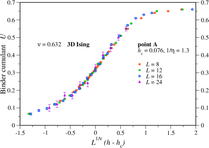
Figure 5: Data collapse of the Binder cumulant (21) for point A at $h_{c}=0.076$, $1/\eta=1.3$ using the 3D Ising exponent $\nu=0.632$ ($z=1$). Data is obtained from continuous-time Monte Carlo simulations at inverse temperature $\beta=2L$.

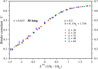
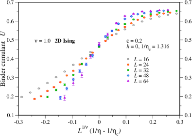
Figure 6: Data collapse of the Binder cumulant (21) for $h=0$ and $(1/\eta)_{c}=1.316$, obtained from discrete-time Monte Carlo simulations with $\epsilon=0.2$ and $\beta=3$. Left panel: 3D exponent $\nu=0.632$. Right panel: 2D exponent $\nu=1$.

In Fig. 5, we show an example of such data collapse for $h_{c}=0.076$, $1/\eta=1.3$. It is very hard to obtain the phase boundary close to the Ising CQCP using the continuous-time algorithm because the gap becomes very small and one needs to simulate very low temperatures to obtain any meaningful results. We believe that the phase transition is in the 3D Ising universality class with $z=1$ and $\nu=0.632$ at any point on the phase boundary for finite values of $h$.

IV.2 Instability of the 2D Ising point to Trotter errors

In this subsection, we show that the Ising CQCP is unstable even to the Trotter discretization errors. The imaginary time direction can be discretized in $N=\beta/\epsilon$ slices and using the Suzuki-Trotter decomposition, one maps the 2D quantum model onto the 3D (Ising-type) classical model with inter-layer couplings given by the diagonal couplings in Eq. (20) and the intra-layer ferromagnetic coupling $K^{\tau}=-1/2\ln\tanh\epsilon\Gamma$, where $\Gamma=1/\eta^{4}$ is the strength of the quantum transverse field. $K^{\tau}$ diverges in the limit $\epsilon\to 0$.

This approach is often used to obtain the critical exponents when simulations using the continuous-time algorithm are cumbersome. The exponents obtained by discrete-time and continuous-time methods should have the same values for stable fixed points. However, in our case, the 2D Ising point is unstable and we obtain the 3D Ising exponents in discrete time indicating that there is a flow to the 3D Ising fixed point, see Fig. 6. Thus we may have the case when quantum-to-classical mapping fails. In principle, one should recover 2D exponents in the limit $\epsilon\to 0$. We are unable to do this because the third direction becomes very large for small $\epsilon$ and Monte Carlo simulations become quite impractical.

IV.3 PIGS simulations

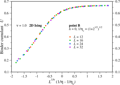
Figure 7: Data collapse of the Binder cumulant (21) for point B at $h=0$, $(1/\eta)_{c}=(1+\sqrt{2})^{1/2}$ using the 2D Ising exponent $\nu=1$. The numerical data is obtained from continuous-time PIGS Monte Carlo simulations at $\beta=0.4$.

The continuous-time quantum Monte Carlo simulations around the Ising CQCP become very slow because we use local updates in the spatial direction. To prove that the transition at $h=0$ and $\eta=\eta_{c}$ is indeed in the 2D Ising universality class, we perform quantum Monte Carlo simulations by using the path integral ground state (PIGS) Monte Carlo algorithm.pigs In the PIGS algorithm, one uses a variational wave function and tries to project the ground state wave function. In our case, the ground state is known exactly (strictly speaking, the wave function given in Eq. (2) is not the exact ground state in discrete time but becomes one in the limit $\epsilon\to 0$). Thus simulations can be performed at any temperature if one uses the continuous-time algorithm. We choose $1/T=0.4$. This temperature is low enough to have substantial quantum dynamics and to avoid trivial classical simulations of the Ising model that one effectively has at high temperatures. Figure. 7 shows the data collapse of the Binder cumulant (21) with the 2D Ising correlation length exponent. The 2D Ising exponents can also be recovered using the PIGS Monte Carlo algorithm in discrete time at small enough values of $\epsilon$, not shown.

V Conformal quantum critical lines with constant and varying $z$

The two-dimensional classical Ising model at its critical point provides a simple example of a conformal field theory. All the scaling dimensions can be determined, and one finds that there are no marginal perturbations possible. However, by coupling two critical Ising models together, one finds a theory with an exactly marginal operator, leading to a line of renormalization group (RG) fixed points. If the Ising spins are on the same lattice, this is called the Ashkin-Teller model, while if they are on interpenetrating square lattices, this is called the eight-vertex model.Baxbook In equivalent fermionic language, this amounts to coupling two Majorana fermions together with an exactly marginal four-fermion term.

This richer behavior persists in quantum theories with RK Hamiltonians. We review below how this coupling yields two conformal quantum critical lines.AFF For any given point on one line one can map its correlators – given in terms of the underlying classical theory – to those of a point on the other line. Thus the equal-time correlators in the quantum theory have the same behavior at these two related points. This, however, is no guarantee that the quantum theories have the same dynamical behavior. Indeed we will show in the following that the dynamical behavior turns out to be quite different.

On one of these lines, the quantum six-vertex model, the model has a height description and so has a $U(1)$ symmetry. Thus one expects the quantum Lifshitz theory to describe the scaling limit, and indeed we see numerically that $z$ remains $2$ all along this line. The second conformal quantum critical line includes the case where the two Ising CQCPs are decoupled. Thus there is no $U(1)$ symmetry, and as we saw above, $z$ is not 2. However, these two critical lines intersect, and so necessarily $z$ cannot remain at the Ising value along this line. We present numerical work that indicates that $z$ indeed varies continuously along this line.

In fact, an argument adapted from Ref. AFF, suggests that $z\geq 2$ for a CQCP. By relating the stress tensor of the two-dimensional conformal field theory describing the ground state of the CQCP to deformations of the quantum Hamiltonian, it is argued that terms in the latter can only depend on space via the Laplacian, e.g. terms like $(\nabla^{2}\varphi)^{2}$ in the quantum Lifshitz theory. In general there is no scalar field, but the argument still suggests that the usual Lorentz-invariant terms in the effective action yielding $z=1$ are absent. Moreover, fields in a unitary conformal field theory necessarily have non-negative dimension, so acting with the dimension-2 Laplacian gives a field of dimension at least 2. This suggests that $z\geq 2$ for CQCPs where the underlying conformal field theory is unitary, as for the theories considered here. It would be interesting to make this argument more precise; we indeed find that this bound is satisfied for all the CQCPs we study.

V.1 The model

As before, we study the Ising models in their domain wall/loop formulation, so that the degrees of freedom live on the links of the lattice. We place these models on two interpenetrating square lattices (i.e. on both a square lattice and its dual). Then the quantum model has a four-state system on each face of the doubled lattice, illustrated in Figure 8. The sites on the original lattice are labeled by solid circles, while the dual lattice sites are labeled by the open circles, so the figures applies to half the faces; the others are given by a rotation. The constraint (14) is required on all sites on the doubled lattice, assuring that neither type of loop branches or ends.

Figure 8: The four configurations in the coupled deformed toric codes, and their weights in the ground state.

The phase diagram of the coupled model is well understood, because the corresponding classical model is equivalent to the eight-vertex model .Baxbook This can be seen by first reverting to the original Ising spins on the doubled lattice, and then drawing the domain walls on the dual lattice to the doubled lattice. The four configurations in Fig. 8 then become the eight vertices of the zero-field eight-vertex model. The counting is as follows. There are of course 16 possible configurations of four Ising spins around a plaquette. One can flip all the spins on the lattice of solid circles without changing the configurations in Fig. 8. One can do the same for the lattice of open circles. Flipping the spins on both lattices does not change the eight-vertex configuration, but flipping the spins on say the solid lattice does. Thus the 16 different Ising spin configurations correspond to the eight different configurations in the eight-vertex model and the four different configurations in Fig. 8. In the standard eight-vertex model language, the four configurations in Figure 8 have weights $c,a,b$ and $d$, respectively. To make the connection with coupled Ising domain walls more apparent, we set $c=1/\eta$ and $d=\eta x$ and $a=b=1$.

The RK Hamiltonian with this ground state is therefore the same as that of Ref. AFF, . It is comprised of a sum over 2 by 2 blocks just like the Ising case. The off-diagonal terms flip all the solid lines around a plaquette on the dual lattice, or flip the dotted lines around a plaquette on the original lattice. The 2 by 2 block thus acts on four faces surrounding each point on the doubled lattice. Let $n_{c}$ be the number of these four faces which are empty, and $n_{d}$ be the number of crossings in these four. Likewise, let $\widetilde{n}_{c}$ and $\widetilde{n}_{d}$ be the number of empty faces and crossings in the flipped configuration. Then the diagonal term for each site is given by $c^{2\widetilde{n}_{c}}d^{2\widetilde{n}_{d}}$, i.e. what enters is the number of crossings and empty faces in the flipped configuration. Each 2 by 2 block is then

$$\mathcal{Q}_{i} = c^{\widetilde{n}_{c}+n_{c}}d^{\widetilde{n}_{d}+n_{d}}\begin{pmatrix}c^{\widetilde{n}_{c}-n_{c}}d^{\widetilde{n}_{d}-n_{d}}&-1\\ -1&c^{n_{c}-\widetilde{n}_{c}}d^{n_{d}-\widetilde{n}_{d}}\\ \end{pmatrix}$$ (22)

$$= \begin{pmatrix}c^{2\widetilde{n}_{c}}d^{2\widetilde{n}_{d}}&-c^{n_{c}+\widetilde{n}_{c}}d^{n_{d}+\widetilde{n}_{d}}\\ -c^{n_{c}+\widetilde{n}_{c}}d^{n_{d}+\widetilde{n}_{d}}&c^{2n_{c}}d^{2n_{d}}\\ \end{pmatrix}\,,$$

where $c=1/\eta$ and $d=\eta x$ as before. The reason for the prefactor as compared to Ref. AFF, is to ensure that the terms remain finite in the $c\to 0$ and $d\to 0$ limits. The fact that $n_{c}+n_{d}+\widetilde{n}_{c}+\widetilde{n}_{d}=4$ can be used to rewrite the off-diagonal terms if desired.

V.2 Constant $z=2$ along the $U(1)$ symmetric line

One critical line occurs when there is a $U(1)$ symmetry, on the quantum six-vertex line. This $U(1)$ symmetry arises when $x=0$, i.e. the dotted and solid lines are never permitted to cross in the ground state, so that there is a three-state system on each face. The symmetry becomes apparent by rewriting the degrees of freedom in terms of an integer-valued “height” $h$ at each site of doubled lattice. Heights on adjacent sites differ by one. The solid lines in Fig. 8 represent domain walls between heights on the original lattice, while the dashed lines are domain walls between heights on the dual lattice. On a disc or sphere, this definition is unique up to an overall shift $h\to h+n$ or a sign flip $h\to-h$. (When $x\neq 0$, one can consistently assign only ${\mathbb{Z}}_{2}$-valued heights, i.e. Ising variables, consistently.)

Thus this height has the same properties as the field $\varphi$ in the quantum Lifshitz model discussed in Sec. II.1, and it is natural to identify $h$ with $\varphi$ in the continuum limit. However, as with the XY model, the classical model is not critical for all values of $\eta$; a Kosterlitz-Thouless transition occurs at $c=2$. Thus for $x=0$, the model is critical for any $\eta\geq 1/\sqrt{2}$. This critical line should be described by the quantum Lifshitz model. The exponents in equal-time correlators will depend on $\eta$, but we should have $z=2$ all along this line. We have checked this explicitly for one point at $x=0$ and $\eta=1/\sqrt{2}$.

A subtlety in taking the $x=0$ limit is that crossings are not forbidden with this Hamiltonian. Rather, they become fixed defects. However, except in peculiar special cases all such defects have a non-zero gap, and so can be ignored in the scaling limit. Another thing to note is that there are extra ground states on the torus in the $x=0$ limit. These are the analog of tilted states in the dimer case, where the height is not periodic around a cycle of the torus. In the language of dashed and solid loops, these result from configurations where the loops around a cycle alternate between dashed and solid. Two neighboring loops of the same type around a cycle can annihilate, but loops of different type cannot: they lie on different sets of links. Thus when crossing is forbidden, there is no way for non-contractible loops of alternating type to annihilate.

V.3 Continuous variation of $z$ along the ${\mathbb{Z}}_{2}$-symmetric line

Figure 9: Two configurations differ by a single plaquette flip. Thin lines denote empty faces and thick lines denote nonempty faces. Here $n_{c}=2$, $n_{d}=0$, $\tilde{n}_{c}=0$, and $\tilde{n}_{d}=2$, see text.

The second critical lineAFF in the quantum eight-vertex model, which does not have a $U(1)$ symmetry, is parametrized by $c^{2}=d^{2}\pm 2$, or

$$x_{c}^{2}=\frac{1}{\eta^{4}}\mp\frac{2}{\eta^{2}}\ .$$ (23)

We will refer to this line as the “${\mathbb{Z}}_{2}$ critical line”. For $x_{c}=0$ this line meets the $U(1)$ critical line discussed in the previous section, and we thus expect a dynamical critical exponent $z=2$ at this point. However, when $\eta^{2}=\sqrt{2}-1$ on the ${\mathbb{Z}}_{2}$ line, we recover the case of two decoupled Ising models corresponding to $x_{c}=1$. For this second point we thus expect a dynamical critical exponent of $z\approx 2.17$ as previously obtained in extensive numerical simulations of the dynamics of the 2d Ising model,LandauBinder see also Fig. 3. As a result, one is led to expect that the dynamical critical exponent is varying (continuously) along the ${\mathbb{Z}}_{2}$ critical line. This might not be surprising since it is known that all static critical exponents (of the equal-time correlators) are continuously varying along the ${\mathbb{Z}}_{2}$ and $U(1)$ critical lines. Thus it might be natural to expect that in the absence of additional symmetries all critical exponents, including $z$, are continuously varying along such a critical line.

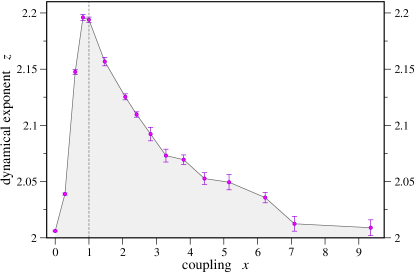
Figure 10: The dynamical exponent $z$ as a function of $x$ along the critical line. The dashed line indicates the coupling $x=1$ of the case of two decoupled classical Ising models. Error bars shown correspond to the statistical errors of the numerical fit described in Appendix A. For a discussion of systematic errors see Appendix B.

To calculate the variation of the dynamical critical exponent along the ${\mathbb{Z}}_{2}$ critical line, we again perform classical Monte Carlo simulations. The off-diagonal part of the Hamiltonian of the two coupled deformed toric codes is more complicated compared with the single deformed toric code. To work out the transition matrix, we note that the weights before and after update are $w({\cal C})=(x\eta^{2})^{2n_{d}}\eta^{2\tilde{n}_{c}+2\tilde{n}_{d}}$ and $w({\cal C}^{\prime})=(x\eta^{2})^{2\tilde{n}_{d}}\eta^{2n_{c}+2n_{d}}\,,$ respectively. An example of such an update is shown in Fig. 9. Given the off-diagonal matrix element $Q_{ij}=-(1/\eta)^{n_{c}+\tilde{n}_{c}}(x\eta)^{n_{d}+\tilde{n}_{d}},$ it is easy to obtain the transition matrix

$$W_{{\cal C},{\cal C}^{\prime}}=w({\cal C}^{\prime}).$$

This is indeed a legitimate transition matrix since $0\leq w\leq 1$.

In Fig. 10, we show our numerical estimates of the dynamical critical exponent $z$ as a function of the coupling $x$. The point $x=0$ is the special point where the two critical lines meet. Here $z=2$ (within error bars), as it remains all along the critical line with $U(1)$ symmetry ($x=0$ and $\eta\geq 1\sqrt{2}$). Moving along the ${\mathbb{Z}}_{2}$ critical line with increasing coupling $x$, we see that $z$ indeed varies continuously. The dynamical exponent has a non-monotonic behavior with an increase up to a maximum of $2.196$ close to the Ising point ($x=1$) and a decrease down towards $z=2$ as $x$ goes to infinity. We note that there might be small systematic errors, which are discussed in Appendix B in detail, because the system sizes are not large enough for the majority of points in Fig. 10.

The contrasting observation that the dynamical critical exponent does not change along the $U(1)$ critical line – despite continuously varying equal-time correlators – suggests that this additional $U(1)$ symmetry protects the dynamical critical exponent $z=2$. This is in line with the general classification of Hohenberg and Halperin ,HH within which the ${\mathbb{Z}}_{2}$ symmetric line is in the Model A dynamical symmetry class (absence of any conservation law), and the $U(1)$ symmetric line in the Model B dynamical symmetry class (presence of a conservation law).

VI Discussion

We have studied the dynamics of a number of conformal quantum critical points. We explored the Ising CQCP in depth, showing that its dynamics are equivalent to classical dynamics. We also showed that it is quite unstable, and that by perturbing with the usual nearest-neighbor interaction it can be continuously connected to the conventional Lorentz-invariant Ising transition in 2+1 dimensions. By studying two coupled deformed toric codes, we illustrated how different dynamics can result in different values of $z$, even when the equal-time correlators are the same.

There are several interesting directions for future research. At the beginning of Sec. V we discussed two quantum-critical lines, one possessing $U(1)$ symmetry and the other possessing only ${\mathbb{Z}}_{2}$ symmetry. These two lines intersect at one point at which the dynamical critical exponent is $z=2$. This point, not surprisingly, has enhanced symmetry. For example, the equal-time correlations are known to possess an $SU(2)$ symmetry. Moreover, the physics should be in the same universality class as the loop models studied in Ref. Troyer08, . The coupling constant moving one along the ${\mathbb{Z}}_{2}$ line away from this intersection point with $SU(2)$ symmetry must be an exactly marginal perturbation which generates a line of fixed points for both statics and dynamics. In particular, by performing perturbation theory in this coupling constant around the $SU(2)$ point, one expects to be able to obtain analytic expressions for the deviation of the dynamic critical exponent from $z=2$.

It would be interesting to explore whether the quantum critical line recently postulated Vidal10 for the toric code model in a multicomponent magnetic field bears some relation to our results. It was found Vidal10 that along this line the product $z\nu$ of dynamical critical exponent and correlation exponent appears to vary from approximately $0.69$ to $1$. The most likely interpretation of those results might be in terms of a crossover between a conformal quantum critical point with $z=2$ and correlation exponent $\nu=1/2$ – corresponding to the $x\to\infty$ limit of the ${\mathbb{Z}}_{2}$ critical line in the quantum eight-vertex model studied in this manuscript – and a Lorentz-invariant (2+1) dimensional multicritical point. Such a scenario would be akin to the crossover discussed in detail in Sec. IV.

One may further ask if it is possible to define a quantum dynamics of RK type based on classical stochastic dynamics as discussed in this paper, for (2+1) dimensional systems supporting non-Abelian statistics. A case in point is the Levin-Wen model,LevinWen which can be viewedNaturePhysicsPaper ; BurnellSimon as a ‘lattice regularization’ of (2+1)-dimensional doubled SU(2) Chern-Simons theory at level $k=3$, possessing anyon excitations with non-Abelian exchange statistics. Indeed, the ground state $|\Psi\rangle$ of this model in the simplest non-abelian (Fibonacci) case can be described in a geometric form similar to Eq. (2). Such a description is found by using the results of Ref. Fidkowski, to rewrite the Fibonacci Levin-Wen model in terms of the quantum net model of Refs. FendleyFradkin, ; FendleyPaperNets, . Here, the configurations ${\cal C}$ describe configurations of so-called ”nets”, which provide an orthonormal basis as in Eq. (1). A key difference with Eq. (2) is that $\sqrt{w({\cal C})}$ is replaced by a real wavefunction of the configurations ${\cal C}$ which takes on both positive and negative values. (The lack of positivity of the wavefunction (”sign problem”) may be a general feature of systems supporting excitations with non-Abelian statistics.) This property prevents one from constructing a quantum dynamics of RK type for the Fibonacci Levin-Wen model by using a stochastic relaxational dynamics of a suitable classical statistical model, as we did in Sec. II.3.

Nevertheless, there is a classical 2D statistical mechanics model which arises naturally from the ground state $|\Psi\rangle$ of the Fibonacci Levin-Wen model, and gives rise to a CQCP.FendleyFradkin ; FendleyPaperNets By tuning the weight per unit length of net just as we did in this manuscript, the (2+0)-dimensional classical partition function obtained from the wave function $|\Psi\rangle$, $Z=\langle\Psi|\Psi\rangle$ is critical. $Z$ is now a sum of non-negative Boltzmann weights because only the square of the wavefunction appears due to the orthonormality of the basis. By Hastings’ theorem, the quantum model must therefore be critical. This classical critical point is in the universality class of the $(2+0)$-dimensional conformal minimal model with central charge $c=14/15$ (or in the language of Ref. FendleyFradkin, ; FendleyPaperNets, , the $Q$-state Potts model with $Q=(5+\sqrt{5})/2$).FootnoteNaturePhysOnePlusOne Such a conformal field theory is knownZamolodchikovMulticritical to be described by a classical Boltzmann weight arising from Landau-Ginzburg theory, precisely of the type described above Eq. (12). Were it not for the ”sign problem” mentioned above, one could proceed to study the dynamic critical exponent $z$ for this conformal quantum critical point along the lines of the present manuscript.

Appendix A Numerical calculation of the dynamical critical exponent

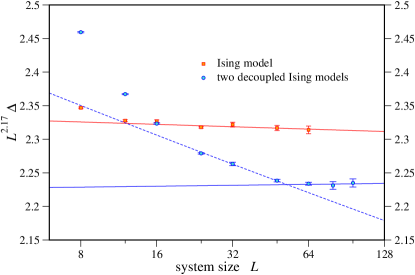
Figure 11: Four times the gap of Hamiltonian (18) and the gap of Hamiltonian (22) ($x=1$) at the critical point $\eta_{c}$ as a function of the system size. The gaps are multiplied by $L^{2.17}$ to make the difference between the two curves clearly visible. The gaps of the two decoupled Ising models show very strong system size dependence. Fitting the curve from $L=24$ to $L=64$ gives $z=2.192(3)$ (indicated by the dashed line), whereas fitting the curve from $L=64$ to $L=96$ gives $z=2.170(4)$ (indicated by the solid line) as for the single Ising model.

In this Appendix, we describe our numerical method. To extract the dynamical critical exponent $z$, we use the finite size scaling of the gap $\Delta\propto L^{-z}$ at the critical point, where $L$ is the linear system size. The gap can be obtained from the autocorrelation function of classical Monte Carlo simulations by ensuring that the off-diagonal part of the Monte Carlo transition matrix is proportional to the off-diagonal part of a Hamiltonian Henley97 (see also Sec. II.3). Strictly speaking, the Hamiltonian is symmetric but the transition matrix $W_{{\cal C},{\cal C}^{\prime}}$ is not. The following matrix is symmetric and has the same eigenvalues as $W_{{\cal C},{\cal C}^{\prime}}$: Henley97

$$\tilde{W}_{{\cal C},{\cal C}^{\prime}}=w({\cal C})^{1/2}W_{{\cal C},{\cal C}^{\prime}}w({\cal C}^{\prime})^{-1/2},$$

where $w({\cal C})$ and $w({\cal C}^{\prime})$ are the statistical weights of the configurations before and after update. If the transition matrix $\tilde{W}$ is proportional to the Hamiltonian:

$$\tilde{W}=1-cH,$$

where $c$ is the coefficient of proportionality, then the gap of the Hamiltonian is related to the autocorrelation time $\tau_{A}$ of some observable $A$ as

$$\Delta=\frac{1-e^{1/\tau_{A}}}{c},$$

where $\tau_{A}$ is measured in Monte Carlo time units. The autocorrelation time $\tau_{A}$ can be obtained by fitting the autocorrelation function to an exponential function (at long enough Monte Carlo time to make sure that the contribution from the other modes is negligible).

We perform Monte Carlo simulations as follows. We simulate a classical model corresponding to the quantum Hamiltonian for different system sizes $L$. Typically the largest system size is $L=64$. We measure the autocorrelation time of the magnetization for Ising-like models and the autocorrelation time of a product of two dimers separated by a distance of $L/2$ for the dimer model. The dynamical exponent is calculated as described in the previous paragraph. Typically we perform 25 independent runs for every point and the error bars are obtained by using the jackknife method.

Appendix B Size dependence of the gap in the deformed toric code model

We note that at the decoupling point $x=1$ of the deformed toric code model, describing two decoupled Ising models, the gap shows very strong system size dependence reaching the asymptotic exponential form only at large system sizes. In Fig. 11, we show the gaps of this model and the ordinary Ising model as functions of the system size. The dynamical critical exponent of the two decoupled Ising models is $z=2.192(3)$ if we fit the curve from $L=24$ to $L=64$ and $z=2.170(4)$ if we fit the curve from $L=64$ to $L=96$. The latter value is in agreement with that for the ordinary Ising model.Nightingale The origin of this strong system size dependence might be tracked back to the additional prefactor $c^{\widetilde{n}_{c}+n_{c}}d^{\widetilde{n}_{d}+n_{d}}$ in Hamiltonian (22) as compared to the ordinary Ising Hamiltonian (18). This prefactor might give rise to slightly modified dynamics for small system sizes. Typically the largest system size in our Monte Carlo simulations is $L=64$ for small values of $x$ and $L=48$ for large values of $x$. Assuming that the gaps for all points in Fig. 10 have strong system size dependence, we may conclude that each point in Fig. 10 might have a (small) systematic error.

References

- (1) P. C. Hohenberg and B. I. Halperin, Rev. Mod. Phys. 49, 435 (1977).
- (2) D. Rokhsar and S. A. Kivelson, Phys. Rev. Lett. 61, 2376 (1988).
- (3) R. Moessner and S. L. Sondhi, Phys. Rev. Lett. 86, 1881 (2001).
- (4) M. B. Hastings, Phys. Rev. B 69, 104431 (2004); Europhys. Lett. 70, 824 (2005).
- (5) We note that Hamiltonians that are the sum of local projectors and that have at least one zero-energy ground state are sometimes referred to as “frustration-free”, in particular in literature concerned with quantum information. Distinguishing such Hamiltonians is a good idea, since many interesting Hamiltonians can be written as a sum over local projectors (e.g. the spin-1/2 Heisenberg model), but typically there is no state annihilated by all of them. Unfortunately, calling these “frustration-free” can lead to confusion, since part of the physics interest in such models is that they often arise from spin models with a large amount of frustration! For example, the classical dimer model on the honeycomb lattice is equivalent to the zero-temperature antiferromagnetic Ising model on the triangular lattice; the dimers themselves correspond to the frustrated bonds .MS2 For this reason, we continue to refer to such Hamiltonians as RK Hamiltonians.
- (6) R. Moessner and S. L. Sondhi, Phys. Rev. B 63, 224401 (2001).
- (7) E. Ardonne, P. Fendley, and E. Fradkin, Ann. Phys. 310, 493 (2004).
- (8) C. L. Henley, J. Stat. Phys. 89, 483 (1997).
- (9) P. Ghaemi, A. Vishwanath, and T. Senthil, Phys. Rev. B 72, 024420 (2005).
- (10) R. J. Baxter, Exactly Solved Models in Statistical Mechanics (Academic, London, 1982).
- (11) C. L. Henley, J. Phys.: Condens. Matter 16, 891 (2004).
- (12) C. Castelnovo, C. Chamon, C. Mudry, and P. Pujol, Ann. Phys. 318, 316 (2005); Phys. Rev. B 73, 144411 (2006).
- (13) D. P. Landau and K. Binder, A Guide to Monte Carlo Simulations in Statistical Physics (Cambridge University Press, 2000).
- (14) S. Trebst, P. Werner, M. Troyer, K. Shtengel, and C. Nayak, Phys. Rev. Lett. 98, 070602 (2007).
- (15) J. Vidal, S. Dusuel, and K. P. Schmidt, Phys. Rev. B 79, 033109 (2009).
- (16) I. S. Tupitsyn, A. Kitaev, N. V. Prokof ev, and P. C. E. Stamp, Phys. Rev. B 82, 085114 (2010)
- (17) S. Dusuel, M. Kamfor, R. Orus, K. P. Schmidt, and J. Vidal, arXiv:1012.1740
- (18) I. Klich, Ann. Phys. 325, 2120 (2010).
- (19) S. Bravyi, M. B. Hastings, and S. Michalakis, J. Math. Phys. 51 093512 (2010); S. Bravyi and M. B. Hastings, arXiv:1001.4363.
- (20) E. Fradkin, D. A. Huse, R. Moessner, V. Oganesyan, and S.L. Sondhi, Phys. Rev. B 69, 224415 (2004).
- (21) A. Vishwanath, L. Balents, and T. Senthil, Phys. Rev. B 69, 224416 (2004).
- (22) M.E. Fisher and J. Stephenson, Phys. Rev. 132, 1411 (1963).
- (23) A. Laeuchli, S. Capponi, F.F. Assaad, J. Stat. Mech. P01010 (2008).
- (24) see e.g.: J. Zinn-Justin, “Quantum Field Theory and Critical Phenomena” (Clarendon Press, Oxford, 1993).
- (25) Recent applications of such a supersymmetric formulation of stochastic dynamics to a variety of problems include Ref. RefDijkgraafOrlandoReffert, .
- (26) R. Dijkgraaf, D. Orlando, and S. Reffert, Nucl. Phys. B 824, 365 (2010).
- (27) A.Y. Kitaev, Ann. Phys. 303, 2 (2003).
- (28) C. Castelnovo and C. Chamon, Phys. Rev. B 77, 054433 (2008).
- (29) See, for example, M. P. Nightingale and H. W. J. Blöte, Phys. Rev. B 62, 1089 (2000).
- (30) B. I. Halperin, Phys. Rev. B 8, 4437 (1973).
- (31) H. W. J. Blöte and Y. Deng, Phys. Rev. E 66, 066110 (2002).
- (32) H. Rieger and N. Kawashima, Eur. Phys. J. B 9, 233, (1999).
- (33) A. Sarsa, K. Schmidt, and W. Magro, J. Chem. Phys. 113, 1366 (2000).
- (34) M. Troyer, S. Trebst, K. Shtengel, and C. Nayak, Phys. Rev. Lett. 101, 230401 (2008).
- (35) M. A. Levin and X.-G. Wen, Phys. Rev. B 71, 045110, (2005).
- (36) C. Gils, S. Trebst, A. Kitaev, A. W. W. Ludwig, M. Troyer, and Z. Wang, Nature Physics 5, 834 (2009).
- (37) F. J. Burnell and S.H. Simon, Ann. Phys. 325, 2550 (2010).
- (38) L. Fidkowski, M. Freedman, C. Nayak, K. Walker, and Z. Wang, Commun. Math. Phys. 287, 805 (2009).
- (39) P. Fendley and E. Fradkin, Phys. Rev. B 72, 024412 (2005).
- (40) P. Fendley, Ann. Phys. 323, 311 (2008).
- (41) Whereas this conformal field theory (CFT) describes the critical ground state wave function of the Fibonacci Levin Wen model which resides in (2+0) dimensions, a conformal field theory of the same central charge was found by entirely different techniques for the quantum dynamics of the same Levin Wen model when spatially confined to quasi one dimensional geometry, and tuned across a quantum critical point by a generic term in the Hamiltonian. This CFT thus describes a (1+1) dimensional system, and has dynamic critical exponent , analogous to the (2+1) dimensional Ising model described in Sec. IV. A priori, there is of course no obvious reason that the same CFT should arise in these (2+0) and (1+1) dimensional limits.
- (42) A. B. Zamolodchikov, Sov. J. Nucl. Phys. 44, 530 (1986).