The quasi-periodic doubling cascade in the transition to weak turbulence

Abstract

The quasi-periodic doubling cascade is shown to occur in the transition from regular to weakly turbulent behaviour in simulations of incompressible Navier-Stokes flow on a three-periodic domain. Special symmetries are imposed on the flow field in order to reduce the computational effort. Thus we can apply tools from dynamical systems theory such as continuation of periodic orbits and computation of Lyapunov exponents. We propose a model ODE for the quasi-period doubling cascade which, in a limit of a perturbation parameter to zero, avoids resonance related problems. The cascade we observe in the simulations is then compared to the perturbed case, in which resonances complicate the bifurcation scenario. In particular, we compare the frequency spectrum and the Lyapunov exponents. The perturbed model ODE is shown to be in good agreement with the simulations of weak turbulence. The scaling of the observed cascade is shown to resemble the unperturbed case, which is directly related to the well known doubling cascade of periodic orbits.

1 Introduction

In the absence of boundaries the incompressible Navier-Stokes equations are symmetric under rotations, translations and reflections. If we impose a subgroup of symmetries on the solutions we reduce the number of degrees of freedom in simulations of the flow. In the early days of numerical simulation such reduction by symmetry was used to probe into turbulent flow, revealing structures such as the Taylor-Green vortex [1]. Kida [2] put forward what is probably the maximal reduction still allowing for turbulent flow. The corresponding flow is called high symmetric and was used to study flow statistics at moderate to high Reynolds number [3, 4, 5].

As computers have grown considerably since then, those results may be reproduced today in simulations without any special symmetry. However, reduction by symmetry can still be a useful approach when going to ever higher Reynolds number, requiring higher resolution of the models, and when applying tools of dynamical systems theory to turbulence.

Recently considerable effort has been made to apply continuation and bifurcation analysis to fluid dynamical problems, see e.g. [6, 7]. If this could be done at realistic resolution the results could prove a valuable complement to statistical analysis of direct numerical simulation. At the moment the maximum number of degrees of freedom tackled successfully is of order $10^{4}$. Given that the simulation of turbulent flow at moderate Reynolds number requires a number of degrees of freedom in the order of $10^{6}$, reduction by symmetry can be successfully applied.

Here, we examine the transition from regular to weakly turbulent motion in high symmetric flow. Exploiting the divergence free condition in addition to the symmetry we gain a factor of about $300$ with respect to general, non symmetric flow and a factor of $3/2$ with respect to earlier work on high symmetric flow in terms of the number of degrees of freedom. Thus we can analyse the transition using continuation of periodic orbits and computation of Lyapunov exponents, using the direct method for integration rather then the pseudo-spectral method.

In addition to the Ruelle-Takens scenario, reported on previously [8], we find that a cascade of quasi-periodic doubling bifurcations, otherwise knows as torus doubling bifurcations, occurs in the transition to weak turbulence. To the author’s best knowledge this is the first time this bifurcation sequence is found in Navier-Stokes flow at realistic truncation level. In order to relate the numerical results to theoretical predictions we propose a model Ordinary Differential Equation (ODE) for this cascade. In contrast to model equations studied previously [9, 10] these equations, based on a fixed time smooth suspension of the Hénon map, display a complete cascade with a fixed frequency ratio of the bifurcating tori in the limit of a perturbation parameter to zero. If we introduce a slight perturbation in the model ODE the bifurcation cascade is interrupted, as it is in the simulations of weak turbulence. Also, the frequency spectrum at the onset of chaos and the dependence of the leading Lyapunov exponents on the bifurcation parameter in the simulations is shown to be very similar those of the perturbed model ODE.

To within the accuracy of the numerics, the scaling of the cascade is shown to agree with that of the unperturbed model ODE, which is known theoretically. When looking at the leading Lyapunov exponents a difference becomes apparent: in the unperturbed model ODE the largest two nonzero exponents become equal on an open interval in parameter space in between successive doubling bifurcation points, whereas in the perturbed model ODE, and also in the flow simulations, they remain separate. This difference might by caused by the crossing of resonance tongues or other codimension one phenomena in which the stable torus loses normal hyperbolicity. A thorough study of the model ODE with finite perturbation might yield an explanation.

2 The vorticity equation for high symmetric flow

Consider an incompressible fluid in a periodic box $0<x_{1},x_{2},x_{3}\leq 2\pi$. In terms of the Fourier representation of velocity and vorticity,

$$\mathbf{v}=\mbox{i}\sum_{\mathbf{k}}\tilde{\mathbf{v}}(\mathbf{k})\mbox{e}^{\mbox{\small i}\mathbf{k}\cdot\mathbf{x}} \qquad{\mbox{\boldmath${\omega}$}}=\sum_{\mathbf{k}}\tilde{\mbox{\boldmath${\omega}$}}(\mathbf{k})\mbox{e}^{\mbox{\small i}\mathbf{k}\cdot\mathbf{x}}$$ (1)

we have

$$\frac{\mbox{d}}{\mbox{d}t}\tilde{\omega}_{i}(\mathbf{k}) = \epsilon_{ijk}k_{j}k_{l}\,\widetilde{v_{k}v_{l}}-\nu k^{2}\tilde{\omega}_{i}(\mathbf{k})$$ (2)

$$k_{i}\tilde{u}_{i} = 0$$ (3)

$$\tilde{\omega}_{i}(\mathbf{k}) = -\epsilon_{ijk}k_{j}\tilde{v}_{k}(\mathbf{k})$$ (4)

where $\nu$ is the kinematic viscosity, $\epsilon_{i,j,k}$ is the permutation symbol and the tilde denotes the Fourier transform. In terms of the standard norm energy and enstrophy are given by

$$E=\frac{1}{2}\|\mathbf{v}\|^{2} \qquad Q=\frac{1}{2}\|\mathbf{\omega}\|^{2}$$ (5)

respectively. Now consider the following discrete symmetry operations: $S_{i}$, reflections in the planes $V_{i}$ given by $x_{i}=\pi$ and $R_{i}$, rotations over $\pi/2$ radiants about the lines $l_{i}:x_{j}=\pi/2\>\mbox{for $j\neq i$}$. If the flow is invariant under these operations only one out of three components of vorticity in a volume fraction $1/4^{3}$ needs to be computed to determine the flow on the periodic domain. Figure 1 gives an impression of the symmetries. We call a flow invariant under $S_{i}$ and $R_{i}$, first described by Kida [2], high symmetric.

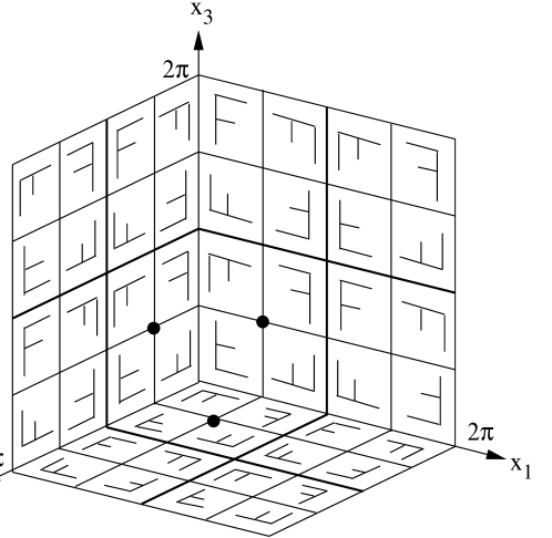
Figure 1: The structure of high symmetry. F represents the state on a face of a box with edges of length $\pi/2$. Reproduced from [2].

Symmetry operations $S_{i}$ and $R_{i}$ introduce linear relations between the Fourier components of vorticity. First of all we have

$$\tilde{\omega}_{1}(k_{1},k_{2},k_{3})=\tilde{\omega}_{2}(k_{3},k_{1},k_{2})=\tilde{\omega}_{3}(k_{2},k_{3},k_{1})$$ (6)

so that we may consider only one component. This scalar function is even or odd in its arguments:

$$\tilde{\omega}_{1}(k_{1},k_{2},k_{3}) = \tilde{\omega}_{1}(-k_{1},k_{2},k_{3})=$$ (7)

$$-\tilde{\omega}_{1}(k_{1},-k_{2},k_{3})=-\tilde{\omega}_{1}(k_{1},k_{2},-k_{3})$$

and finally we have

$$\tilde{\omega}_{1}(k_{1},k_{2},k_{3})=\left\{\begin{array}[]{ll}-\tilde{\omega}_{1}(k_{1},k_{3},k_{2})&\mbox{for $k_{1}$ and $k_{2}$ and $k_{3}$ even,}\\ \tilde{\omega}_{1}(k_{1},k_{3},k_{2})&\mbox{for $k_{1}$ and $k_{2}$ and $k_{3}$ odd,}\\ 0&\mbox{otherwise.}\end{array}\right.$$ (8)

We consider a cubic truncation, i.e. $|k_{1,2,3}|\leq N$. Relations (6-8) reduce the number of independent Fourier modes of vorticity by a factor of $192$ in the leading order, that is $N^{3}$. This reduction was exploited by Kida et al.[3, 4] to investigate scaling laws at moderate to high Reynolds number. In the present work we exploit the divergence free condition for vorticity to further reduce the number of modes. With the aid of equation (6) it reads

$$k_{1}\tilde{\omega}_{1}(k_{1},k_{2},k_{3})+k_{2}\tilde{\omega}_{1}(k_{2},k_{3},k_{1})+k_{3}\tilde{\omega}_{1}(k_{3},k_{1},k_{2})=0$$ (9)

Taking maximal advantage of relations (6-9) we consider only Fourier components of $\omega_{1}$ in the fundamental domain $\{\mathbf{k}\in\mathbb{Z}^{3}|k_{3}>k_{2},k_{3}\geq k_{1},k_{1}\geq 0,k_{2}>0,k_{3}\leq N\}$. The number of independent modes is reduced by a factor of $288$ in the leading order.

These components satisfy the following equation

$$\frac{\mbox{d}}{\mbox{d}t}\tilde{\omega}_{1}(k_{1},k_{2},k_{3}) = k_{2}k_{3}(\tilde{S}(k_{3},k_{1},k_{2})-\tilde{S}(k_{2},k_{3},k_{1}))$$ (10)

$$+k_{1}k_{2}\tilde{T}(k_{2},k_{3},k_{1})-k_{3}k_{1}\tilde{T}(k_{3},k_{1},k_{2})$$

$$+(k_{2}^{2}-k_{3}^{2})\tilde{T}(k_{1},k_{2},k_{3})-\nu k^{2}\tilde{\omega}_{1}(k_{1},k_{2},k_{3})$$

where $\tilde{S}$ and $\tilde{T}$ are the Fourier transforms of

$$S(x_{1},x_{2},x_{3}) = v_{1}(x_{1},x_{2},x_{3})^{2}$$

$$T(x_{1},x_{2},x_{3}) = v_{1}(x_{2},x_{3},x_{1})v_{1}(x_{3},x_{1},x_{2})$$ (11)

and

$$k^{2}\tilde{v}_{1}=k_{2}\tilde{\omega}_{1}(k_{3},k_{1},k_{2})-k_{3}\tilde{\omega}_{1}(k_{2},k_{3},k_{1})$$ (12)

Energy in supplied by fixing the low order odd mode $\tilde{\omega}_{1}(1,1,3)=-3/8$. Thus we obtain a family of dynamical systems with one parameter, $\nu$, and a number of degrees of freedom given by

$$n(N)=\left\{\begin{array}[]{ll}\frac{2}{3}\left(\frac{N}{2}\right)^{3}+\frac{1}{2}\left(\frac{N}{2}\right)^{2}-\frac{7}{6}\frac{N}{2}-1&\mbox{if $N$ is even}\\ \frac{2}{3}\left(\frac{N-1}{2}\right)^{3}+\frac{3}{2}\left(\frac{N-1}{2}\right)^{2}-\frac{1}{6}\left(\frac{N-1}{2}\right)-1&\mbox{if $N$ is odd.}\end{array}\right.$$ (13)

3 Numerical considerations

In performing time integrations we avoid the use of a pseudo-spectral method, commonly employed for three dimensional simulations of Navier-Stokes. Up to a truncation level of $N=25$ ($n=1365$) the direct method is not exceedingly slow due to the reduction of the number of degrees of freedom described above and yields easy access to the Jacobian for integration of the variational equations. Also, the direct integration code can easily be run in parallel, distributing the computation of the components of the vector field over any number of processors. For higher truncation levels, at which storage of the nonlinear interaction coefficients requires huge memory space, it is mandatory to use a pseudo spectral method, as described in [3], even though it does not exploit the divergence free condition (9). For time integration a seventh to eight order Runge-Kutta-Felbergh scheme with adaptive step size is employed. As many of the results presented here are based on rather long time integrations it important to keep the error tolerance low. We have checked energy conservation at zero forcing and viscosity using the high order and the fourth order Runge-Kutta schemes. For realistic $\mbox{O}(1)$ levels of the energy, an integration time $\Delta t=10^{3}$ and a fixed error tolerance $\delta E=10^{-9}$ the step size required for the fourth order scheme is about ten times smaller then the average step size using the high order scheme. As the high order method needs thirteen evaluations of the vector field at each time step, against four for the low order scheme, it is more efficient.

Below simulations are performed with a viscosity in the range $0.005<\nu<0.01$ and the truncation level fixed to $N=15$ ($n=300$). We computed the energy and the enstrophy, as well as Taylor’s micro-scale Reynolds number, $R_{\lambda}$, and Kolmogorov’s dissipation length scale, $\eta$, defined by

$$R_{\lambda}=\sqrt{\frac{10}{3}}\frac{E}{\nu\sqrt{Q}} \qquad\eta=\sqrt[4]{\frac{\nu^{2}}{2Q}}$$ (14)

The dimensionless number $\eta N$ indicates if the resolution is high enough in numerical simulations. If $\eta N\sim 1$ the truncation error is considered negligible. At the fist transition to chaos, the focus of this paper, we have $\eta N\approx 0.8$. The band average energy spectrum is shown in figure 2(left). In order to make sure that the results presented below do not depend critically on the truncation level we repeated some of the computations, in particular the location of the quasi-periodic bifurcation points described in section 5, at $N=21$ ($n=814$). The qualitative behaviour remains the same as the bifurcation points shift slightly to lower viscosity. For this truncation level we have $\eta N\approx 1$ at the first transition point. The band-averaged energy spectrum is shown in figure 2(right). At the small scales an exponential decay is visible, indicating that our numerical results are reliable.

Figure 2: Band-averaged energy spectra near the first transitions to chaos, described in section 5. Obtained from an integration of $300$ time units, log-linear scale in normalised units. Left: truncation level $N=15$, right: $N=21$.

Periodic orbits are continued in the viscosity as fixed points of a Poincaré map, using the arclength method as described in [11]. This method is time consuming because of the integration of the linearised equations. However, running the code in parallel this is no obstacle.

4 Transitions to chaos

Figure 3: Limit point diagram of high symmetric flow simulations. Iterates of the Poincaré map, obtained from an integration of length $\Delta t=1000$, are drawn for each parameter value. Transient motion is discarded and the step size of the parameter is set to $\delta\nu=1\cdot 10^{-4}$. The last point of each integration is the initial point at the next parameter value, starting at the stable periodic orbit at $\nu=0.0105$. Visible is the transition I$\rightarrow$II from periodic to quasi periodic, II$\rightarrow$III to chaotic, III$\rightarrow$IV back to periodic, IV$\rightarrow$V to quasi periodic and V$\rightarrow$VI to chaotic/turbulent. In region III the behaviour alternates between chaotic and two or three periodic while the spatial structure of the flow remains simple.

Figure 4: Branches of periodic orbits of high symmetric flow, truncated at $N=15$. Solid lines denote stable branches and dashed lines unstable branches. Bifurcation points are marked SN for saddle-node, NS for Neimark-Sacker and H for Hopf. The roman number refer to the stable periodic behaviour as seen in the limit point diagram, figure 3.

For large viscosity an equilibrium state is the global attractor in our simulations of high symmetric flow. At $\nu\approx 0.0113$ a Hopf bifurcation occurs in which a stable periodic orbit is created. To get an impression of the transitions from periodic to chaotic motion we computed a limit point diagram in the range $0.01>\nu>0.005$ of the Poincaré map on the coordinate plane given by $\tilde{\omega}(0,2,4)=-0.05$. In this range the time average micro-scale Reynolds number varies from $R_{\lambda}\approx 50$ to $R_{\lambda}\approx 27$, indicating that the aperiodic behaviour can be classified as weak turbulence, fully developed turbulence sets in around $\nu\approx 0.004$ and $R_{\lambda}\approx 60$ in high symmetric flow. The limit point diagram is shown in figure 3. Two parameter ranges with periodic behaviour can be seen: one around $\nu=0.01$ and one around $\nu=0.0068$. A continuation of these periodic orbits in parameter $\nu$ is shown in figure 4. The branch which is stable around $\nu=0.0068$ does not bifurcate from an equilibrium at high viscosity. Both branches become unstable in a Neimark-Sacker bifurcation. Directly beyond these bifurcation points we expect the behaviour to be quasi periodic, and indeed invariant circles appear in the Poincaré section, figure 3. The breakdown of these invariant tori gives rise to chaos. The torus created at $\mbox{NS}_{2}$ displays a quasi-periodic Hopf bifurcation and thus the Ruelle-Takens scenario to chaos is followed, as reported in [8]. The torus created at $\mbox{NS}_{1}$ displays a quasi-periodic doubling bifurcation which turns out to be the first of a cascade, discussed in detail in section 5.

The fundamental frequencies of the tori created at $\mbox{NS}_{1,2}$ have a physical interpretation. The higher frequency, $\omega_{1}\approx 2.6$ is set by the large eddy overturning time, estimated as $T=l/U\approx 2.3$ where $U\approx 0.9$ is the root mean square velocity and $l=\sqrt[3]{\pi^{3}/3}$ is the characteristic length scale given that by symmetries $S_{i}$, the planes $x_{1,2,3}=\pi$ are impermeable and by symmetries $R_{i}$ the velocity field has a three fold rotational symmetry around the main diagonal $x_{1}=x_{2}=x_{3}$. The lower frequency, $\omega_{2}\approx 0.26$, corresponds to a modulation of the amplitude of the energy. It is also present in fully developed turbulence with high symmetry and can be though of as a retaining time scale of anomalously high energy. The dynamics on these time scales is illustrated by the isosurface of enstrophy shown in figure 5. On the short time scale, $T$, patches of high vorticity are generated on the main diagonal and off the diagonal in triples related by the three fold rotational symmetry. These patches converge to the origin and to the center of the $2\pi$-periodic box, points of special symmetry. On the longer time scale the overall amplitude of this process is modulated. Note, that the patches of high vorticity do not have the elongated, tubular shape typical of developed turbulence.

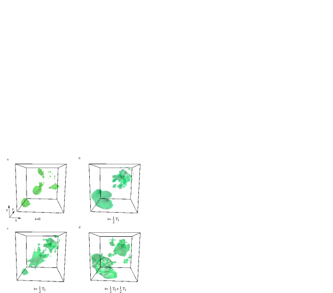
Figure 5: Isosurface of enstrophy during quasi-periodic behaviour corresponding to figure 6a. Edges of length $\pi$, taken from the $2\pi$-periodic domain and isosurface level set to eight times the spatio-temporal average. The main diagonal is an axis of three-fold rotational symmetry. The time step between a and b (c and d) is half the short period $T_{1}=2\pi/\omega_{1}$ and from a to c (b to d) half the long period $T_{2}=2\pi/\omega_{2}$.

5 The quasi-periodic doubling cascade

In figure 6 six Poincaré plots are shown beyond bifurcation point $\mbox{NS}_{1}$. The torus “doubles” at least four times (a-e) before a chaotic attractor appears with a shape very similar to the doubled torus.

Such sequences of torus doubling bifurcations have been observed both numerically, e.g. in severe truncations of the Navier-Stokes equations [17] and in a periodically driven low-order atmosphere model [18], and experimentally, e.g. in electronic circuits [15, 16] and have also been studied in connection to strange non chaotic attractors [19]. In these examples chaotic behaviour is observed after two or three doublings. In our system we find four doublings, after which quasi-periodic motion is very hard to distinguish from aperiodic motion numerically.

The observation of incomplete quasi-periodic doubling cascades led to the introduction of simple models which highlight the similarity to the well known periodic doubling cascade [9, 10]. In these models an infinite cascade can only be observed in a limit of the parameters were the vector field can be decomposed into a three dimensional vector field which exhibits a period doubling cascade and a constant rotation. Away from this limit the stable torus is more fragile after each bifurcation and the cascade is interrupted.

In order to see why the cascade is interrupted, we need to investigate the quasi-periodic doubling bifurcation in detail. Rigorous bifurcation theorems for bifurcating invariant tori were formulated by Broer et al [12, 13]. They include the bifurcation shown here, in which a torus loses stability and a new stable torus is created with one fundamental frequency half that of the original torus. However, the bifurcation theorem is given for a one parameter family of tori that satisfy a non resonance condition on the fundamental frequencies. If the fundamental frequencies of the torus become resonant normal hyperbolicity is lost and persistence under parameter variations is not guaranteed. We have only one parameter in our system and the fundamental frequencies depend on it continuously. As we vary the parameter we cut through a Cantor set of values at which the torus is normally hyperbolic. Thus, the loss of normal hyperbolicity through resonance is a possible mechanism for the interruption of the cascade.

However, the resonances we pass through, i.e. the Arnold’ tongues we cross, are of fairly high order as we find for the fundamental frequencies at $\mbox{NS}_{1}$ that $\omega_{1}\approx 10\omega_{2}$. Recently an algorithm for the continuation of invariant tori was developed that “steps over” such high order resonances without a problem, and in fact this algorithm was tested on a system that exhibits a cascade of quasi-periodic doublings [14]. In this paper it is pointed out that in the absence of a non resonance condition the notion of a quasi-periodic bifurcation point itself is unclear, as no normally hyperbolic torus exists in a whole interval in parameter space. On one side of this interval we observe the stable single torus and on the other side the stable doubled torus. This interval turns out to be small compared to the numerical resolution of our simulations, a step size in the viscosity of about $\delta\nu\approx 10^{-7}$.

Apart form resonances there are other mechanism that can interrupt the cascade. Stagliano et al. [19], for instance, concluded that the cascade was interrupted when the stable torus loses smoothness and collides with an unstable parent torus. In reference [18] a strikingly complicated, yet incomplete picture is sketched of the mechanisms that can interrupt the cascade.

Figure 6: Poincaré sections in the plane $\omega(0,2,4)=-0.05$, projected onto the modes $\omega(2,2,4)$ and $\omega(3,1,3)$. Four quasi-periodic doublings are shown in (a-e) and the resulting chaotic attractor in (f).

Figure 7: Frequency spectrum of the energy just beyond bifurcation point $\mbox{D}_{3}$ around the widely separated frequencies $\omega_{1,2}$. Note the peaks due to the doubling bifurcations around $\omega_{2}$ and the resonance peaks around $\omega_{1}$.

In order to interpret our numerical results, let us formulate a new model ODE for the quasi-periodic doubling cascade. Models studied before [9, 19] were based on the logistic map and cannot be regarded as the Poincaré map of a smooth flow. Our starting point is the Hénon map.

Let $\mathcal{H}_{s}(x,y)$ be a family of Hénon maps on $\mathbb{R}^{2}$ which exhibits a period doubling cascade. Let $\bar{s}_{i}$ be the period doubling bifurcation point at which a stable $2^{i}$-periodic point is created and let $\lim_{i\rightarrow\infty}\bar{s}_{i}=s_{c}$. Let $\phi_{t}(x,y,u;s)$ be a smooth fixed time suspension of $\mathcal{H}_{s}$ on $\mathbb{R}^{2}\times S$ so that $\phi_{1}(x,y,0;s)=(\mathcal{H}_{s}(x,y),0)$. The flow $\phi_{t}$ is generated by an autonomous vector field, denoted here by $f_{1}\partial_{x}+f_{2}\partial_{y}+\partial_{u}$. In appendix A explicit expressions are given as formulated in [20]. Finally, we add a second periodic variable and a coupling proportional to $\epsilon$:

$$\dot{x} =f_{1}(x,y,u;s)+\epsilon h_{1}(v)\qquad\dot{u} =1$$

$$\dot{y} =f_{2}(x,y,u;s)+\epsilon h_{2}(v)\qquad\dot{v} =\omega+\epsilon g(x,y)$$ (15)

with $\mathbf{h}:S\rightarrow\mathbb{R}^{2}$, $g:\mathbb{R}^{2}\rightarrow\mathbb{R}$ and $\omega$ irrational. For $\epsilon=0$ the flow on $\mathbb{R}^{2}\times S\times S$ is given by $\psi_{t}(x,y,u,v;s)=(\phi_{t}(x,y,u;s),v_{0}+\omega t)$ and we know that

1. At $s=\bar{s}_{i}$ a stable torus with fundamental frequencies $1/2^{i}$ and $\omega$ is created.

2. The quasi-periodic doubling bifurcations accumulate on zero with the same scaling as for the period doubling cascade, thus for the bifurcation points we find that $\lim_{i\rightarrow\infty}(s_{i}-s_{i-1})/(s_{i+1}-s_{i})=\delta$, where $\delta=4.669\ldots$, the Feigenbaum constant.

3. The Lyapunov exponents of the attracting torus are determined by the Floquet multipliers of the corresponding periodic points of $\mathcal{H}_{s}$. Therefore the leading nonzero exponent should be equal to the second exponent on a open interval contained in each interval $(\bar{s}_{i},\bar{s}_{i+1})$.

For finite $\epsilon$ the second fundamental frequency will depend on $s$ continuously and resonance points will be passed through on the way to the accumulation point $s=s_{c}$.

In the following we compare the model ODE to the simulations of weak turbulence. The damping parameter of the Hénon map is fixed to $j=1/4$. The unperturbed model then displays a doubling cascade with $s_{1}=1.1718\ldots$, $s_{2}=1.7031\ldots$, $s_{3}=1.8144\ldots$ and $s_{c}=1.84525\ldots$. In the perturbed system we fix the second frequency to the golden mean, i.e. $\omega=(\sqrt{5}+1)/2$ and

$$h_{1}(v) = \sin 2\pi v$$

$$h_{2}(v) = 0$$

$$g(x,y) = y$$ (16)

The perturbation parameter is fixed to $\epsilon=0.001$. At this perturbation strength we observe four doubling bifurcations before chaos sets in. In the Poincaré intersection plane given by $v=0$, projected on the $x$ and $y$ variables, the bifurcation sequence looks very similar to the one shown in figure 6.

We have computed the frequency spectrum near the onset of chaos and the (partial) Lyapunov spectrum both for the weak turbulence and for the model ODE. For computation of Lyapunov exponents of the high-symmetric flow we used finite differencing rather than integration of the full linearised system. Integration was done until the zero exponent associated with the direction transversal to the flow and tangent to the torus had converged up to $10^{-4}$.

Figure 8: Left: largest nonzero Lyapunov exponents $\lambda_{1,2}$ as a function of $\nu$ in the quasi-periodic doubling cascade. The first doubling points have been marked $\mbox{D}_{i}$, $i=1,2,3$. Right: enlargement of the regions around $\mbox{D}_{1}$ and $\mbox{D}_{2}$. Note that after the second doubling the Lyapunov exponents do not meet.

Figure 9: Left: largest nonzero Lyapunov exponents $\lambda_{1,2}$ as a function of $s$ for the model ODE (15) with $\epsilon=0.001$. The doubling points have been marked as in figure 8. Right: enlargement of the region around $\mbox{D}_{3,4}$. The bold lines denote the exponents for the perturbed model at $\epsilon=0.001$. For comparison the exponents for the unperturbed case ($\epsilon=0$) are shown with thin lines. Note that the exponents of the perturbed system do no meet between the doubling points.

Turning first to the frequency spectrum we observe that after three doublings bifurcations peaks at frequencies $\omega_{2}/2$, $\omega_{2}/4$ and $\omega_{2}/8$ show up, as well as combination peaks around $\omega_{1}$. Figure 7 shows the spectrum around the fundamental frequencies for the simulations of weak turbulence. A rather similar figure for the model ODE is omitted here. In the case of a period doubling cascade the amplitude ratio $\mu$ between consecutive peaks $\omega/2^{i}$ can be predicted on basis of the scaling constants [21]. We attempted to measure this ratio for the spectrum shown in figure 7 but only the first three peaks can be distilled from these data. These scale roughly by a factor of $\mu=4$, not far from the theoretical prediction for the period doubling case $\mu=4.648\ldots$. The same estimate is obtained for the model ODE. In the case of Poincaré maps, rather then discrete maps, similar deviations from the theory are found.

In figures 8(left) and 9(left) the leading Lyapunov exponents are shown as a function of the bifurcation parameter, i.e. the viscosity $\nu$ for the high-symmetric flow and the parameter $s$ of the Hénon map for the model ODE. From these data we can estimate the locus of the bifurcation points, stressing once more that this notion is ill-defined on a scale smaller then our resolution in parameter space. Thus we find consecutive estimates for the scaling constant $\delta$ as $\delta_{i}=(\bar{\nu}_{i}-\bar{\nu}_{i-1})/(\bar{\nu}_{i+1}-\bar{\nu}_{i})$ or $\delta_{i}=(\bar{s}_{i}-\bar{s}_{i-1})/(\bar{s}_{i+1}-\bar{s}_{i})$:

$$\delta_{1} = 4.64\pm 0.2\ \qquad\delta_{2}=4.88\pm 0.5\qquad\mbox{for high-symmetric flow and}$$

$$\delta_{1} = 4.75\pm 0.05\qquad\delta_{2}=4.63\pm 0.2\qquad\mbox{for the model ODE.}$$

Again, this is compatible with the theory for period doubling cascades, albeit a rough estimate.

In figure 8(right) enlargements around the points $\mbox{D}_{1}$ and $\mbox{D}_{2}$ are shown for the high-symmetric flow simulations. After the first doubling the leading non zero exponents are equal on small interval of order $\delta\nu=10^{-6}$. After the second doubling the leading exponents neither cross nor become equal. This result was confirmed by integration of the full linearised equations at several points in the parameter range where the leading exponents attain their minimal distance. The parameter range between the third and fourth doublings is too small to see whether the exponents meet. In this range we record the passage through a high order resonance which does not destroy the torus.

In figure 9(right) an enlargement is shown of the Lyapunov exponents of the model ODE around the doubling points $\mbox{D}_{3}$ and $\mbox{D}_{4}$. For comparison, the exponents of the unperturbed model, computed from the Hénon map itself, have been drawn with thin lines. Again the Lyapunov exponents do not become equal in between doubling points. The step size has been taken as small as $\delta s=1\cdot 10^{-5}$. Apparently, the slightly perturbed model ODE yields the same behaviour of the leading Lyapunov exponents as the simulations of high-symmetric flow.

For now we have no explanation for the absence of crossing or equal leading Lyapunov exponents in between doubling points. As noted before, the invariant tori are structurally stable only on a fractal domain of the parameter and bifurcations might go unnoticed when monitoring Lyapunov exponents with finite step size for the parameter. A more thorough understanding could be obtained by a continuation of the invariant torus itself and by further study of the model ODE (15), which is the topic of future research.

6 Conclusion

We have investigated the transition from stationary to disordered behaviour in simulations of high symmetric flow. In combination with the symmetry the divergence free condition was exploited to reduce the number of degrees of freedom by a factor of about $300$ with respect to simulations of general periodic Navier-Stokes flow, a gain of $30\%$ compared to earlier work [2]-[5],[8]. This allowed us to investigate the bifurcation scenario in detail and at realistic truncation level.

Along with the Ruelle-Takens scenario, the quasi-periodic doubling cascade occurs as a route to weak turbulence. By means of Poincaré sections, power spectra and Lyapunov exponents we have shown that this cascade bears close resemblance to the well known doubling cascade for periodic orbits. We observe four doublings after which quasi-periodic behaviour is very hard to distinguish from chaotic behaviour numerically. In previous work on the quasi-periodic doubling cascade, both numerical and experimental, chaos is reported to set in after two or three doublings [15, 17, 16]. The fact that we see more doublings might be due to the widely separate fundamental frequencies of the bifurcating tori in our system, as is the case in recent work by Schilder et al[14].

In order to make the notion of a quasi-periodic doubling cascade precise we have proposed a model ODE, equations (15), such that in the limit of a perturbation parameter $\epsilon\downarrow 0$ the correspondence to the periodic doubling cascade is exact. The scaling of the first steps of the observed quasi-periodic doubling cascade agrees with the prediction of the unperturbed equations (15). Looking at the leading nonzero Lyapunov exponents, however, a difference between the perturbed model ODE and the high-symmetric flow simulations on one side, and the unperturbed model ODE on the other side, becomes apparent. In the perturbed model ODE and in the simulations the two largest nonzero exponents remain separate in between doublings, or at least no crossing is found with a small but finite step size in the parameter. An explanation might follow from a detailed study of the model ODE (15) with nonzero perturbation. Other interesting questions would be if the scaling laws of the doubling cascade are influenced by the perturbation and how many steps of the cascade can be observed given the ratio of fundamental frequencies and the strength of the perturbation.

The solutions presented here, in particular the bifurcating tori, are solutions of the truncated three dimensional Navier-Stokes equations on a periodic domain. They might, however, prove to be unstable to asymmetric perturbations. It is therefore uncertain whether the quasi-periodic doubling cascade can be observed in periodic flow without any symmetries imposed. It does, however, occur at low Reynolds number, at which asymmetric perturbations might be damped. Even at such low Reynolds number, the simulation of general three dimensional flow, and the bifurcation analysis as presented here, remains a formidable task.

Appendix A An explicit suspension of the Hénon map

Explicit expressions for a vector field that yields a fixed time, smooth suspension of the Hénon map were given by Mayer-Kress and Haken [20]. Here we repeat the essential definitions in a the notation of the model ODE 15.

The Hénon map is given by

$$\mathcal{H}_{s}\left(\begin{array}[]{c}x\\ y\end{array}\right) = \left(\begin{array}[]{c}y+F(x;s)\\ -jx\end{array}\right)$$ (21)

$$F(x;s) = 1-sx^{2}$$ (22)

In order to define the function $\mathbf{f}(x,y,u;s)$ we need to introduce the following auxiliary functions:

$$\xi(u) = (3-2u)u^{2}$$

$$\eta(u) = 1+u\ln j-(2\ln j+3)u^{2}+(2+\ln j)u^{3}$$

$$G(\xi,\eta) = \frac{1}{\xi^{2}+\eta^{2}}\left\{\xi^{\prime}\eta-\xi\eta^{\prime}-\xi\eta\left(\ln j-2\frac{\xi\xi^{\prime}+\eta\eta^{\prime}}{\xi^{2}+\eta^{2}}\right)\right\}$$

$$H(\xi,\eta) = \frac{1}{\xi^{2}+\eta^{2}}\left\{(\xi^{\prime}\xi+\eta^{\prime}\eta)\frac{\xi^{2}-\eta^{2}}{\xi^{2}+\eta^{2}}+\eta^{2}\ln j\right\}$$

$$X(x,y) = j^{-u}(\eta x-\xi y)$$ (23)

where the primes denote differentiation with respect to $u$. Suppressing the explicit dependence on $u$ in the right hand side we have

$$\mathbf{f}(x,y,u;s)=\left(\begin{array}[]{cc}H(\xi,\eta)&G(\xi,\eta)\\ G(\eta,\xi)&H(\eta,\xi)\end{array}\right)\left(\begin{array}[]{c}x\\ y\end{array}\right)+F(X(x,y);s)\left(\begin{array}[]{c}\xi\xi^{\prime}\\ \xi^{\prime}\eta\end{array}\right)$$ (24)

References

- [1] Brachet M E, Meiron D I, Orszag S A, Nickel B G, Morf R H and Frisch U 1983 Small-scale structure of the Taylor-Green vortex J.Fluid Mech. 130 411-452.
- [2] Kida S 1985 Three-dimensional periodic flows with high-symmetry J. Phys. Soc. Japan 54 2132–2136.
- [3] Kida S and Murakami Y 1989 Statistics of velocity gradients in turbulence at moderate Reynolds number Fluid.Dyn.Res. 4 347–370.
- [4] Kida S and Murakami Y 1987 Kolmogorov similarity in freely decaying turbulence Phys.Fluids 30 2030–2039.
- [5] Boratav O N and Pelz B P 1997 Structures and structure functions in the inertial range of turbulence Phys. Fluids 9 1400–1415.
- [6] Lust K, Roose D, Spence A and Champneys A R 1998 An adaptive Newton-Picard algorithm with subspace iteration for computing periodic solutions SIAM J.Sci.Comput. 19 1188-1209.
- [7] Sánchez J, Net M, García-Archilla B and Simó C. 2003 Newton-Krylov continuation of periodic orbits for Navier-Stokes flows J.Comput.Phys. in press.
- [8] Kida S, Yamada M and Ohkitani K 1989 A route to chaos and turbulence Physica D 37 116–125.
- [9] Kaneko K 1986 Collapse of tori and genesis of chaos in dissipative systems, World Scientific, Singapore.
- [10] Arnéodo A, Coullet P H and Spiegel E A 1983 Cascade of period doublings of tori Phys. Lett. A 94 1–5.
- [11] Simó C 1989 On the analytical and numerical approximation of invariant manifolds Modern Methods in Celestial Mechanics, Proceedings of the 13th spring school on astrophysics in Goutelas Edition Frontières, Gift-sur Yvette, France. Available via http://www.maia.ub.es/dsg/2004/index.html
- [12] Broer H W, Huitema G B and Takens F. 1990 Unfoldings of quasi-periodic tori Mem. AMS 83(421) 1–82.
- [13] Braaksma B L J, Broer H W and Huitema G B 1990 Toward a quasi-periodic bifurcation theory Mem. AMS 83(421) 83–175.
- [14] Schilder F, Osinga H M and Vogt W 2004 Continuation of quasi-periodic invariant tori Applied nonlinear dynamics preprint 2004.11 University of Bristol.
- [15] Anishenko V S 1990 Complex oscillations in simple systems, Nauka, Moscow.
- [16] Zhong G-Q, Chai W W and Chua L O 1998 Torus-doubling bifurcations in four mutually coupled Chua’s circuits IEEE Trans. Circuits Syst. I 45 186–193.
- [17] Franceschini V 1983 Bifurcation of tori and phase locking in a dissipative system of differential equations Phys. D 6 285–304.
- [18] Broer H W, Simó C and Vitolo R 2002 Bifurcations and strange attractors in the Lorenz-84 climate model with seasonal forcing Nonlinearity 15 1205–1267.
- [19] Stagliano J J, Wersinger J-M and Slaminka E E 1996 Doubling bifurcations of destroyed tori Phys. D 92 164–177.
- [20] Mayer-Kress G and Haken H 1987 An explicit construction of a class of suspensions and autonomous differential equations for diffeomorphisms in the plane Commun.Math.Phys. 111 63–74.
- [21] Feigenbaum M J 1980 The transition to aperiodic behaviour in turbulent systems Commun.Math.Phys. 77 65–86.