Estimating Networks With Jumps

Abstract

We study the problem of estimating a temporally varying coefficient and varying structure (VCVS) graphical model underlying nonstationary time series data, such as social states of interacting individuals or microarray expression profiles of gene networks, as opposed to i.i.d. data from an invariant model widely considered in current literature of structural estimation. In particular, we consider the scenario in which the model evolves in a piece-wise constant fashion. We propose a procedure that minimizes the so-called TESLA loss (i.e., temporally smoothed L1 regularized regression), which allows jointly estimating the partition boundaries of the VCVS model and the coefficient of the sparse precision matrix on each block of the partition. A highly scalable proximal gradient method is proposed to solve the resultant convex optimization problem; and the conditions for sparsistent estimation and the convergence rate of both the partition boundaries and the network structure are established for the first time for such estimators.

1 Introduction

Networks are a fundamental form of representation of relational information underlying large, noisy data from various domains. For example, in a biological study, nodes of a network can represent genes in one organism and edges can represent associations or regulatory dependencies among genes. In a social analysis, nodes of a network can represent actors and edges can represent interactions or friendships between actors. Exploring the statistical properties and hidden characteristics of network entities, and the stochastic processes behind temporal evolution of network topologies is essential for computational knowledge discovery and prediction based on network data.

In many dynamical environments, such as a developing biological system, it is often technically impossible to experimentally determine the network topologies specific to every time point in a discrete time series. Resorting to computational inference methods, such as extant structural learning algorithms, is also difficult because for every model unique to a single time point, there exist as few as only a single snapshot of the nodal states distributed accordingly to the model in question. In this paper, we consider an estimation problem under a particular dynamic context, where the model evolves piecewise constantly, i.e., staying structurally invariant during unknown segments of time, and then jump to a different structure.

A popular technique for deriving the network structure from iid sample is to estimate a sparse precision matrix. The importance of estimating precision matrices with zeros was recognized by (Dempster, 1972) who coined the term covariance selection. The elements of the precision matrix represent the associations or conditional covariances between corresponding variables. Once a sparse precision matrix is estimated, a network can be drawn by connecting variables whose corresponding elements of the precision matrix are non-zero. Recent studies have shown that covariance selection methods based on the penalized likelihood maximization can lead to a consistent estimate of the network structure underlying a Gaussian Markov Random Fields (Fan et al., 2009; Ravikumar et al., 2008). Moreover, a particular procedure for covariance selection known as neighborhood selection, which is built on $\ell_{1}$ norm regularized regression, can produce a consistent estimate of the network structure when the sample is assumed to follow a general Markov Random Field distribution whose structure corresponds to the network in question (Ravikumar et al., 2009; Meinshausen and Bühlmann, 2006; Peng et al., 2009). Specifically, a Markov Random Field (MRF) is a probabilistic graphical model defined on a graph $G=(V,E)$, where $V=\{1,\ldots,p\}$ is a vertex set corresponding to the set of random variables to be modeled (in this paper we call them nodes and variables interchangeably), and $E\subseteq V\times V$ is the edge set capturing conditional indecencies among these nodes. Let $\mathbf{X}=(X_{1},\ldots,X_{p})^{\prime}$ denote a $p$-dimensional random vector, whose elements are indexed by the nodes of the graph $G$. Under the MRF, a pair $(a,b)$ is not an element of the edge set $E$ if and only if the variable $X_{a}$ is conditionally independent of $X_{b}$ given all the rest of variables $X_{V\backslash\{a,b\}}$, $X_{a}\perp X_{b}|X_{V\backslash\{a,b\}}$. A distribution over $\mathbf{X}$ can be defined by taking the following log linear form that makes explicit use of the (presence and absence of edges in the) edge set: $p(\mathbf{X})\propto\exp\{\sum_{(a,b)\in V}\theta_{ab}X_{a}X_{b}\}$. When the elements of the random vector $\mathbf{X}$ are discrete, e.g., $\mathbf{X}\in\{0,1\}^{p}$, the model is referred to as a discrete MRF, sometimes known as an Ising model in statistics physics community; whereas when $\mathbf{X}$ is a continuous vector, the model is referred to as a Gaussian graphical model (GGM) because one can easily show that the $p(\mathbf{X})$ above is actually a multivariate Gaussian. The MRF have been widely used for modeling data with graphical relational structures over a fixed set of entities (Wainwright and Jordan, 2008; Getoor and Taskar, 2007). The vertices can describe entities such as genes in a biological regulatory network, stocks in the market, or people in society; while the edges can describe relationships between vertices, for example, interaction, correlation or influence.

The statistical problem we concern in this paper is to estimate the structure of the Gaussian graphical model from observed samples of nodal states in a dynamic world. Traditional methods handle this problem with the assumption that the samples are iid. Let $\mathcal{D}=\{\mathbf{x}_{1},\ldots,\mathbf{x}_{n}\}$ be an independent and identically distributed sample according to a $p$-dimensional multivariate normal distribution $\mathcal{N}_{p}(\mathbf{0},\bm{\Sigma})$, where $\bm{\Sigma}$ is the covariance matrix. Let $\bm{\Omega}:=\bm{\Sigma}^{-1}$ denote the precision matrix, with elements $(\omega_{ab})$, $1\leq a,b\leq p$. Then one can obtain an estimator of the $\bm{\Omega}$ from $\mathcal{D}$ via optimizing a proper statistical loss function, such as likelihood or penalized likelihood. As mentioned earlier, the precision matrix $\bm{\Omega}$ encodes the conditional independence structure of the distribution and the pattern of the zero elements in the precision matrix define the structure of the associated graph $G$. There has been a dramatic growth of interest in recent literature in the problem of covariance selection, which deals with the graph estimation problem above. Existing works range from algorithmic development focusing on efficient estimation procedures, to theoretical analysis focusing on statistical guarantees of different estimators. We do not intend to give an extensive overview of the literature here, but interested readers can follow the pointers bellow. In the classical literature (e.g. Lauritzen, 1996), procedures are developed for small dimensional graphs and commonly involve hypothesis testing with greedy selection of edges. More recent literature estimates the sparse precision matrix by optimizing penalized likelihood (Yuan and Lin, 2007; Fan et al., 2009; Banerjee et al., 2008; Rothman et al., 2008; Friedman et al., 2008; Ravikumar et al., 2008; Guo et al., 2010b; Zhou et al., 2008) or through neighborhood selection (Meinshausen and Bühlmann, 2006; Peng et al., 2009; Guo et al., 2010a; Wang et al., 2009), where the structure of the graph is estimated by estimating the neighborhood of each node. Both of these approaches are suitable for high-dimensional problems, even when $p\gg n$, and can be efficiently implemented using scalable convex program solvers.

Most of the above mentioned work assumes that a single invariant network model is sufficient to describe the dependencies in the observed data. However, when the observed data are not iid, such an assumption is not justifiable. For example, when data consist of microarray measurements of the gene expression levels collected throughout the cell cycle or development of an organism, different genes can be active during different stages. This suggests that different distributions and hence different networks should be used to describe the dependencies between measured variables at different time intervals. In this paper, we are going to tackle the problem of estimating the structure of the GGM when the structure is allowed to change over time. By assuming that the parameters of the precision matrix change with time, we obtain extra flexibility to model a larger class of distributions while still retaining the interpretability of the static GGM. In particular, as the coefficients of the precision matrix change over time, we also allow the structure of the underlying graph to change as well. This semi-parametric generalization of the parametric model is referred to as a varying coefficient varying structure (VCVS) model.

Now, let $\{\mathbf{x}_{i}\}_{i\in[n]}\in\mathbb{R}^{p}$ be a sequence of $n$ independent observations (we use $[n]$ to denote the set $\{1,\ldots,n\}$) from some $p$-dimensional multivariate normal distributions, not necessarily the same for every observation. Let $\{\mathcal{B}^{j}\}_{j\in[B]}$ be a disjoint partitioning of the set $[n]$ where each block of the partition consists of consecutive elements, that is, $\mathcal{B}^{j}\cap\mathcal{B}^{j^{\prime}}=\emptyset$ for $j\neq j^{\prime}$ and $\bigcup_{j}\mathcal{B}^{j}=[n]$ and $\mathcal{B}^{j}=[T_{j-1}:T_{j}]:=\{T_{j-1},T_{j-1}+1,\ldots,T_{j}-1\}$. Let ${\mathcal{T}}:=\{T_{0}=1<T_{1}<\ldots<T_{B}=n+1\}$ denote the set of partition boundaries. We consider the following model

$$\mathbf{x}_{i}\sim\mathcal{N}_{p}(\mathbf{0},\bm{\Sigma}^{j}),\qquad i\in\mathcal{B}^{j},$$ (1)

so that observations indexed by elements in $\mathcal{B}^{j}$ are $p$-dimensional realizations of a multivariate normal distribution with zero mean and the covariance matrix $\bm{\Sigma}^{j}=(\sigma_{ab}^{j})_{a,b\in[p]}$. Let $\bm{\Omega}^{j}:=(\bm{\Sigma}^{j})^{-1}$ denote the precision matrix with elements $(\omega_{ab}^{j})_{a,b\in[p]}$. With the number of partitions, $B$, and the boundaries of partitions, ${\mathcal{T}}$, unknown, we study the problem of estimating both the partition set $\{\mathcal{B}^{j}\}$ and the non-zero elements of the precision matrices $\{\bm{\Omega}^{j}\}_{j\in[B]}$ from the sample $\{\mathbf{x}_{i}\}_{i\in[n]}$. Note that in this work we study a particular case of the VCVS model, where the coefficients are piece-wise constant functions of time. A scenario where the coefficients are smoothly varying functions of time has been considered in Zhou et al. (2008) for the GGM and in Kolar et al. (2010b) and Kolar and Xing (2009) for an Ising model.

If the partitions $\{\mathcal{B}^{j}\}_{j}$ were known, the problem would be trivially reduced to the setting analyzed in the previous work. Dealing with the unknown partitions, together with the structure estimation of the model, calls for new methods. We propose and analyze a method based on time-coupled neighborhood selection, where the model estimates are forced to stay similar across time using a fusion-type total variation penalty and the sparsity of each neighborhood is obtained through the $\ell_{1}$ penalty. Details of the approach are given in $\S 2$.

The model in Eq. (1) is related to the varying-coefficient models (e.g. Hastie and Tibshirani, 1993) with the coefficients being piece-wise constant functions. Varying coefficient regression models with piece-wise constant coefficients are also known as segmented multivariate regression models (Liu et al., 1997) or linear models with structural changes (Bai and Perron, 1998). The structural changes are commonly determined through hypothesis testing and a separate linear model is fit to each of the estimated segments. In our work, we use the penalized model selection approach to jointly estimate the partition boundaries and the model parameters.

Little work has been done so far towards modeling dynamic networks and estimating changing precision matrices. Zhou et al. (2008) develops a nonparametric method for estimation of time-varying GGM, where $\mathbf{x}^{t}\sim\mathcal{N}_{p}(\mathbf{0},\bm{\Sigma}(t))$ and $\bm{\Sigma}(t)$ is smoothly changing over time. The procedure is based on the penalized likelihood approach of Yuan and Lin (2007) with the empirical covariance matrix obtained using a kernel smoother. Our work is very different from the one of Zhou et al. (2008), since under our assumptions the network changes abruptly rather than smoothly. Furthermore, as we outline in $\S$2, our estimation procedure is not based on the penalized likelihood approach. Estimation of time-varying Ising models has been discussed in Ahmed and Xing (2009) and Kolar et al. (2010b). Yin et al. (2008) and Kolar et al. (2010a) studied nonparametric ways to estimate the conditional covariance matrix. The work of Ahmed and Xing (2009) is most similar to our setting, where they also use a fused-type penalty combined with an $\ell_{1}$ penalty to estimate the structure of the verying Ising model. Here, in addition to focusing on GGMs, there is an additional subtle, but important, difference to Ahmed and Xing (2009). In this work, we use a modification of the fusion penalty (formally described in $\S$2) which allows us to characterize the model selection consistency of our estimates and the convergence properties of the estimated partition boundaries, which is not available in the earlier work.

The remaining of the paper is organized as follows. In $\S$2, we describe our estimation procedure and provide an efficient first-order optimization procedure capable of estimating large graphs. The optimization procedure is based on the smoothing procedure of Nesterov (2005) and converges in $\mathcal{O}(1/\epsilon)$ iterations, where $\epsilon$ is the desired accuracy. Our main theoretical results are presented in $\S$3. In particular, we show that the partition boundaries are estimated consistently. Furthermore, the graph structure is consistently estimated on every block of the partition that contains enough samples. Numerical studies showing the finite sample performance of our procedure are given in $\S$4. The proofs of the main results are relegated to $\S$6, with some technical details presented in Appendix.

Notation Schemes:

For clarity, we end the introduction with a summary of the notations used in the paper. We use $[n]$ to denote the set $\{1,\ldots,n\}$ and $[l:r]$ to denote the set $\{l,l+1,\ldots,r-1\}$. We use $\mathcal{B}^{j}$ to denote $j$-th block of the partition ${\mathcal{T}}$. With some abuse of notation, we also use $\mathcal{B}^{j}$ to denote the set $[T_{j-1}:T_{j}]$. The number of samples in the block $\mathcal{B}^{j}$ is denoted as $|\mathcal{B}^{j}|$. For a set $S\subset V$, we use the notation $X_{S}$ to denote the set $\{X_{a}:a\in S\}$ of random variables. We use $\mathbf{X}$ to denote the $n\times p$ matrix whose rows consist of observations. The vector $\mathbf{X}_{a}=(x_{1,a},\ldots,x_{n,a})^{\prime}$ denotes a column of matrix $\mathbf{X}$ and, similarly, $\mathbf{X}_{S}=(\mathbf{X}_{b}\ :\ b\in S)$ denotes the $n\times|S|$ sub-matrix of $\mathbf{X}$ whose columns are indexed by the set $S$ and $\mathbf{X}^{\mathcal{B}^{j}}$ denotes the sub-matrix $|\mathcal{B}^{j}|\times p$ whose rows are indexed by the set $\mathcal{B}^{j}$. For simplicity of notation, we will use $\backslash a$ to denote the index set $[p]\backslash\{a\}$, $\mathbf{X}_{\backslash a}=(\mathbf{X}_{b}\ :\ b\in[p]\backslash\{a\})$. For a vector $\mathbf{a}\in\mathbb{R}^{p}$, we let $S(\mathbf{a})$ denote the set of non-zero components of $\mathbf{a}$. Throughout the paper, we use $c_{1},c_{2},\ldots$ to denote positive constants whose value may change from line to line. For a vector $\mathbf{a}\in\mathbb{R}^{n}$, define $||\mathbf{a}||_{1}=\sum_{i\in[n]}|a_{i}|$, $||\mathbf{a}||_{2}=\sqrt{\sum_{i\in[n]}a_{i}^{2}}$ and $||\mathbf{a}||_{\infty}=\max_{i}|a_{i}|$. For a symmetric matrix $\mathbf{A}$, $\Lambda_{\min}(\mathbf{A})$ denotes the smallest and $\Lambda_{\max}(\mathbf{A})$ the largest eigenvalue. For a matrix $\mathbf{A}$ (not necessarily symmetric), we use $|\!|\!|\mathbf{A}|\!|\!|_{{\infty}}=\max_{i}\sum_{j}|A_{ij}|$. For two vectors $\mathbf{a},\mathbf{b}\in\mathbb{R}^{n}$, the dot product is denoted $\langle{\mathbf{a}},{\mathbf{b}}\rangle=\sum_{i\in[n]}a_{i}b_{i}$. For two matrices $\mathbf{A},\mathbf{B}\in\mathbb{R}^{n\times m}$, the dot product is denoted as $\langle\!\langle{\mathbf{A}},{\mathbf{B}}\rangle\!\rangle=\mathop{\mathrm{tr}}(\mathbf{A}^{\prime}\mathbf{B})$. Given two sequences $\{a_{n}\}$ and $\{b_{n}\}$, the notation $a_{n}=\mathcal{O}(b_{n})$ means that there exists a constant $c_{1}$ such that $a_{n}\leq c_{1}b_{n}$; the notation $a_{n}=\Omega(b_{n})$ means that there exists a constant $c_{2}$ such that $a_{n}\geq c_{2}b_{n}$ and the notation $a_{n}\asymp b_{n}$ means that $a_{n}=\mathcal{O}(b_{n})$ and $b_{n}=\mathcal{O}(a_{n})$. Similarly, we will use the notation $a_{n}=o_{p}(b_{n})$ to denote that $b_{n}^{-1}a_{n}$ converges to $0$ in probability.

Table 1: Summary of symbols used throughout the paper

Symbol	Meaning	Example
$[n]$	used to denote the set $\{1,\ldots,n\}$
$[t_{1}:t_{2}]$	used to denote the set $\{t_{1},t_{1}+1,\ldots,t_{2}-1\}$
$i$	used for indexing related to samples	$\mathbf{x}^{i}$ or $\beta_{\cdot,i}^{a}$
$j,k$	used for indexing related to block	$\bm{\theta}^{a,j}$ or $S_{a}^{k}$
$a,b$	used for indexing nodes in a graph	$a,b\in V$
$G$	the graph consisting of vertices and edges	$G=(V,E)$
$V$	the set of nodes in a graph	$V=[p]$
$E_{i}$	the set of edges at time $i$
$X_{a}$	the component of a random vector $\mathbf{X}$ indexed by the vertex $a$
$\bm{\beta}_{\cdot,i}^{a}$	the vector of regression coefficients for sample $i$
$\bm{\theta}^{a,j}$	the vector of regression coefficients for block $j$
${\mathcal{T}}$	the set of partition boundaries
$\{\tau_{j}\}_{j}$	the set of boundary fractions	$T_{j}=\lfloor n\tau_{j}\rfloor$
$\mathcal{B}^{j}$	an index set for the samples in the partition $j$	$\mathcal{B}^{j}\subset[n]$
$B$	denotes the number of partitions
$S_{a}^{j}$	the set of neighbors of node $a$ in block $j$
$S(\bm{\theta}^{a,j})$	the set of non-zero elements of $\bm{\theta}^{a,j}$
$\bar{S}_{a}^{j}$	the closure of $S_{a}^{j}$	$\bar{S}_{a}^{j}=S_{a}^{j}\cup\{a\}$
$N_{a}^{j}$	nodes not in the neighborhood of the node $a$ in block $j$	$N_{a}^{j}=[p]\backslash\bar{S}_{a}^{j}$
$\backslash a$	the set of all vertices excluding the vertex $a$	$\backslash a=[p]\backslash\{a\}$
$|\cdot|$	cardinality of a set or absolute value
$\bm{\Sigma}$	the covariance matrix
$\sigma_{ab}$	an element of the covariance matrix
$\bm{\Omega}$	the precision matrix
$\omega_{ab}$	an element of the precision matrix
$\langle{\cdot},{\cdot}\rangle$	the dot product	$\langle{\mathbf{a}},{\mathbf{b}}\rangle=\mathbf{a}^{\prime}\mathbf{b}$
$\langle\!\langle{\cdot},{\cdot}\rangle\!\rangle$	the dot product between matrices	$\langle\!\langle{\mathbf{A}},{\mathbf{B}}\rangle\!\rangle=\mathop{\mathrm{tr}}(\mathbf{A}^{\prime}\mathbf{B})$
$\xi_{\min}$	the minimum change between regression coefficient	$||\bm{\theta}^{a,j}-\bm{\theta}^{a,j-1}||_{2}\geq\xi_{\min}$
$\theta_{\min}$	the minimum size of a coefficient	$|\theta_{b}^{a,j}|\geq\theta_{\min}$
$\Delta_{\min}$	the minimum size of a block	$|\mathcal{B}^{j}|\geq\Delta_{\min}$

2 Graph estimation via Temporal-Difference Lasso

In this section, we introduce our time-varying covariance selection procedure, which is based on the time-coupled neighborhood selection using the fused-type penalty. We call the proposed procedure Temporal-Difference Lasso (TD-Lasso). We start by reviewing the basic neighborhood selection procedure, which has previously been used to estimate graphs in, for example, Peng et al. (2009), Meinshausen and Bühlmann (2006), Ravikumar et al. (2009) and Guo et al. (2010a).

We start by relating the elements of the precision matrix $\bm{\Omega}$ to a regression problem. Let the set $S_{a}$ to denote the neighborhood of the node $a$. Denote $\bar{S}_{a}$ the closure of $S_{a}$, $\bar{S}_{a}:=S_{a}\cup\{a\}$, and $N_{a}$ the set of nodes not in the neighborhood of the node $a$, $N_{a}=[p]\backslash\bar{S}_{a}$. It holds that $X_{a}\perp X_{N_{a}}|X_{S_{a}}$. The neighborhood of the node $a$ can be easily seen from the non-zero pattern of the elements in the precision matrix $\bm{\Omega}$, $S_{a}=\{b\in[p]\backslash\{a\}\ :\ \omega_{ab}\neq 0\}$. See Lauritzen (1996) for more details. It is a well known result for Gaussian graphical models that the elements of

$$\bm{\theta}^{a}=\mathop{\mathrm{argmin}}_{\bm{\theta}\in\mathbb{R}^{p-1}}\ \mathbb{E}(X_{a}-\sum_{b\in\backslash a}X_{b}\theta_{b})^{2}$$

are given by $\theta^{a}_{b}=-\omega_{ab}/\omega_{aa}$. Therefore, the neighborhood of a node $a$, $S_{a}$, is equal to the set of non-zero coefficients of $\bm{\theta}^{a}$. Using the expression for $\bm{\theta}^{a}$, we can write $X_{a}=\sum_{b\in S_{a}}X_{b}\theta^{a}_{b}+\epsilon$, where $\epsilon$ is independent of $X_{\backslash a}$.

The neighborhood selection procedure was motivated by the above relationship between the regression coefficients and the elements of the precision matrix. Meinshausen and Bühlmann (2006) proposed to solve the following optimization procedure

$$\hat{\bm{\theta}}^{a}=\mathop{\mathrm{argmin}}_{\bm{\theta}\in\mathbb{R}^{p-1}}\ \frac{1}{n}||\mathbf{X}_{a}-\mathbf{X}_{\backslash a}\bm{\theta}||_{2}^{2}+\lambda||\bm{\theta}||_{1}$$ (2)

and proved that for iid sample the non-zero coefficients of $\hat{\bm{\theta}}^{a}$ consistently estimate the neighborhood of the node $a$, under a suitably chosen penalty parameter $\lambda$.

In this paper, we build on the neighbourhood selection procedure to estimate the changing graph structure in model (1). We use $S_{a}^{j}$ to denote the neighborhood of the node $a$ on the block $\mathcal{B}^{j}$ and $N_{a}^{j}$ to denote nodes not in the neighborhood of the node $a$ on the $j$-th block, $N_{a}^{j}=V\backslash S_{a}^{j}$. Consider the following estimation procedure

$$\hat{\bm{\beta}}^{a}=\mathop{\mathrm{argmin}}_{\bm{\beta}\in\mathbb{R}^{p-1\times n}}\ \mathcal{L}(\bm{\beta})+{\rm pen}_{\lambda_{1},\lambda_{2}}(\bm{\beta})$$ (3)

where the loss is defined for $\bm{\beta}=(\beta_{b,i})_{b\in[p-1],i\in[n]}$ as

$$\mathcal{L}(\bm{\beta}):=\sum_{i\in[n]}\bigg{(}x_{i,a}-\sum_{b\in\backslash a}x_{i,b}\beta_{b,i}\bigg{)}^{2}$$ (4)

and the penalty is defined as

$${\rm pen}_{\lambda_{1},\lambda_{2}}(\bm{\beta}):=2\lambda_{1}\sum_{i=2}^{n}||\bm{\beta}_{\cdot,i}-\bm{\beta}_{\cdot,i-1}||_{2}+2\lambda_{2}\sum_{i=1}^{n}\sum_{b\in\backslash a}|\beta_{b,i}|.$$ (5)

The penalty term is constructed from two terms. The first term ensures that the solution is going to be piecewise constant for some partition of $[n]$ (possibly a trivial one). The first term can be seen as a sparsity inducing term in the temporal domain, since it penalizes the difference between the coefficients $\bm{\beta}_{\cdot,i}$ and $\bm{\beta}_{\cdot,i+1}$ at successive time-points. The second term results in estimates that have many zero coefficients within each block of the partition. The estimated set of partition boundaries

$$\hat{\mathcal{T}}=\{\hat{T}_{0}=1\}\cup\{\hat{T}_{j}\in[2:n]\ :\ \hat{\bm{\beta}}_{\cdot,\hat{T}_{j}}^{a}\neq\hat{\bm{\beta}}_{\cdot,\hat{T}_{j}-1}^{a}\}\cup\{\hat{T}_{\hat{B}}=n+1\}$$

contains indices of points at which a change is estimated, with $\hat{B}$ being an estimate of the number of blocks $B$. The estimated number of the block $\hat{B}$ is controlled through the user defined penalty parameter $\lambda_{1}$, while the sparsity of the neighborhood is controlled through the penalty parameter $\lambda_{2}$.

Based on the estimated set of partition boundaries $\hat{\mathcal{T}}$, we can define the neighborhood estimate of the node $a$ for each estimated block. Let $\hat{\bm{\theta}}^{a,j}=\hat{\bm{\beta}}^{a}_{\cdot,i}$, $\forall i\in[\hat{T}_{j-1}:\hat{T}_{j}]$ be the estimated coefficient vector for the block $\hat{\mathcal{B}}^{j}=[\hat{T}_{j-1}:\hat{T}_{j}]$. Using the estimated vector $\hat{\bm{\theta}}^{a,j}$, we define the neighborhood estimate of the node $a$ for the block $\hat{\mathcal{B}}^{j}$ as

$$\hat{S}_{a}^{j}:=S(\hat{\bm{\theta}}^{a,j}):=\{b\in\backslash a\ :\ \hat{\theta}^{a,j}_{b}\neq 0\}.$$

Solving (3) for each node $a\in V$ gives us a neighborhood estimate for each node. Combining the neighborhood estimates we can obtain an estimate of the graph structure for each point $i\in[n]$.

The choice of the penalty term is motivated by the work on penalization using total variation (Rinaldo, 2009; Mammen and van de Geer, 1997), which results in a piece-wise constant approximation of an unknown regression function. The fusion-penalty has also been applied in the context of multivariate linear regression Tibshirani et al. (2005), where the coefficients that are spatially close, are also biased to have similar values. As a result, nearby coefficients are fused to the same estimated value. Instead of penalizing the $\ell_{1}$ norm on the difference between coefficients, we use the $\ell_{2}$ norm in order to enforce that all the changes occur at the same point.

The objective (3) estimates the neighborhood of one node in a graph for all time-points. After solving the objective (3) for all nodes $a\in V$, we need to combine them to obtain the graph structure. We will use the following procedure to combine $\{\hat{\bm{\beta}}^{a}\}_{a\in V}$,

$$\hat{E}_{i}=\{(a,b)\ :\ \max(|\beta^{a}_{b,i}|,|\beta^{b}_{a,i}|)>0\},\qquad i\in[n].$$

That is, an edge between nodes $a$ and $b$ is included in the graph if at least one of the nodes $a$ or $b$ is included in the neighborhood of the other node. We use the $\max$ operator to combine different neighborhoods as we believe that for the purpose of network exploration it is more important to occasionally include spurious edges than to omit relevant ones. For further discussion on the differences between the min and the max combination, we refer an interested reader to Banerjee et al. (2008).

2.1 Numerical procedure

Finding a minimizer $\hat{\bm{\beta}}^{a}$ of (3) can be a computationally challenging task for an off-the-shelf convex optimization procedure. We propose too use an accelerated gradient method with a smoothing technique (Nesterov, 2005), which converges in $\mathcal{O}(1/\epsilon)$ iterations where $\epsilon$ is the desired accuracy.

We start by defining a smooth approximation of the fused penalty term. Let $\mathbf{H}\in\mathbb{R}^{n\times n-1}$ be a matrix with elements

$$H_{ij}=\left\{\begin{array}[]{cl}-1&\text{if }i=j\\ 1&\text{if }i=j+1\\ 0&\text{otherwise.}\end{array}\right.$$

With the matrix $\mathbf{H}$ we can rewrite the fused penalty term as $2\lambda_{1}\sum_{i=1}^{n-1}||(\bm{\beta}\mathbf{H})_{\cdot,i}||_{2}$ and using the fact that the $\ell_{2}$ norm is self dual (for example, see Boyd and Vandenberghe, 2004) we have the following representation

$$2\lambda_{1}\sum_{i=2}^{n}||\bm{\beta}_{\cdot,i}-\bm{\beta}_{\cdot,i-1}||_{2}=\max_{\mathbf{U}\in\mathcal{Q}}\ \langle\!\langle{\mathbf{U}},{2\lambda_{1}\bm{\beta}\mathbf{H}}\rangle\!\rangle$$ (6)

where $\mathcal{Q}:=\{\mathbf{U}\in\mathbb{R}^{p-1\times n-1}\ :\ ||\mathbf{U}_{\cdot,i}||_{2}\leq 1,\ \forall i\in[n-1]\}$. The following function is defined as a smooth approximation to the fused penalty,

$$\Psi_{\mu}(\bm{\beta}):=\max_{\mathbf{U}\in\mathcal{Q}}\ \langle\!\langle{\mathbf{U}},{2\lambda_{1}\bm{\beta}\mathbf{H}}\rangle\!\rangle-\mu||\mathbf{U}||_{F}^{2}$$ (7)

where $\mu>0$ is the smoothness parameter. It is easy to see that

$$\Psi_{\mu}(\bm{\beta})\leq\Psi_{0}(\bm{\beta})\leq\Psi_{\mu}(\bm{\beta})+\mu(n-1).$$

Setting the smoothness parameter to $\mu={\textstyle\frac{\epsilon}{2(n-1)}}$, the correct rate of convergence is ensured. Let $\mathbf{U}_{\mu}(\bm{\beta})$ be the optimal solution of the maximization problem in (7), which can be obtained analytically as

$$\mathbf{U}_{\mu}(\bm{\beta})=\Pi_{\mathcal{Q}}\left(\frac{\lambda\bm{\beta}\mathbf{H}}{\mu}\right)$$ (8)

where $\Pi_{\mathcal{Q}}(\cdot)$ is the projection operator onto the set $\mathcal{Q}$. From Theorem 1 in Nesterov (2005), we have that $\Psi_{\mu}(\bm{\beta})$ is continuously differentiable and convex, with the gradient

$$\nabla\Psi_{\mu}(\bm{\beta})=2\lambda_{1}\mathbf{U}_{\mu}(\bm{\beta})\mathbf{H}^{\prime}$$ (9)

that is Lipschitz continuous.

With the above defined smooth approximation, we focus on minimizing the following objective

$$\min_{\bm{\beta}\in\mathbb{R}^{p-1\times n}}F(\bm{\beta}):=\min_{\bm{\beta}\in\mathbb{R}^{p-1\times n}}\mathcal{L}(\bm{\beta})+\Psi_{\mu}(\bm{\beta})+2\lambda_{2}||\bm{\beta}||_{1}.$$

Following Beck and Teboulle (2009) (see also Nesterov (2007)), we define the following quadratic approximation of $F(\bm{\beta})$ at a point $\bm{\beta}_{0}$

$$Q_{L}(\bm{\beta},\bm{\beta}_{0}):=\mathcal{L}(\bm{\beta}_{0}) +\Psi_{\mu}(\bm{\beta}_{0})+\langle\!\langle{\bm{\beta}-\bm{\beta}_{0}},{\nabla\mathcal{L}(\bm{\beta}_{0})+\nabla\Psi(\bm{\beta}_{0})}\rangle\!\rangle$$ (10)

$$+\frac{L}{2}||\bm{\beta}-\bm{\beta}_{0}||_{F}^{2}+2\lambda_{2}||\bm{\beta}||_{1}$$

where $L>0$ is the parameter chosen as an upper bounds for the Lipschitz constant of $\nabla\mathcal{L}+\nabla\Psi$. Let $p_{L}(\bm{\beta}_{0})$ be a minimizer of $Q_{L}(\bm{\beta},\bm{\beta}_{0})$. Ignoring constant terms, $p_{L}(\bm{\beta}_{0})$ can be obtained as

$$p_{L}(\bm{\beta}_{0})=\mathop{\mathrm{argmin}}_{\bm{\beta}\in\mathbb{R}^{p-1\times n}}\ \frac{1}{2}\bigg{\|}\bm{\beta}-\Big{(}\bm{\beta}_{0}-\frac{1}{L}\big{(}\nabla\mathcal{L}+\nabla\Psi\big{)}(\bm{\beta}_{0})\Big{)}\bigg{\|}_{F}^{2}+\frac{2\lambda_{2}}{L}\big{\|}\bm{\beta}\big{\|}_{1}.$$

It is clear that $p_{L}(\bm{\beta}_{0})$ is the unique minimizer, which can be obtained in a closed form, as a result of the soft-thresholding,

$$p_{L}(\bm{\beta}_{0})=T\bigg{(}\bm{\beta}_{0}-\frac{1}{L}\big{(}\nabla\mathcal{L}+\nabla\Psi\big{)}(\bm{\beta}_{0}),\frac{2\lambda_{2}}{L}\bigg{)}$$ (11)

where $T(x,\lambda)=\mathop{\mathrm{sign}}(x)\max(0,|x|-\lambda)$ is the soft-thresholding operator that is applied element-wise.

In practice, an upper bound on the Lipschitz constant of $\nabla\mathcal{L}+\nabla\Psi$ can be expensive to compute, so the parameter $L$ is going to be determined iteratively. Combining all of the above, we have the following algorithm.

Algorithm:  Accelerated Gradient Method for Equation (3)

Input: $\mathbf{X}\in\mathbb{R}^{n\times p}$, $\bm{\beta}_{0}\in\mathbb{R}^{p-1\times n}$, $\gamma>1$, $L>0$, $\mu=\frac{\epsilon}{2(n-1)}$

Output: $\hat{\bm{\beta}}^{a}$

Initialize $k:=1$, $\alpha_{k}:=1$, $\mathbf{z}_{k}:=\bm{\beta}_{0}$

repeat

       while $F(p_{L}(\mathbf{z}_{k}))>Q_{L}(p_{L}(\mathbf{z}_{k}),\mathbf{z}_{k})$ do

            $L:=\gamma L$

       $\bm{\beta}_{k}:=p_{L}(\mathbf{z}_{k})$   (using Eq. (11))

       $\alpha_{k+1}:=\frac{1+\sqrt{1+4\alpha_{k}}}{2}$

      $\mathbf{z}_{k+1}:=\bm{\beta}_{k}+\frac{\alpha_{k}-1}{\alpha_{k+1}}\big{(}\bm{\beta}_{k}-\bm{\beta}_{k-1}\big{)}$

until convergence

$\hat{\bm{\beta}}^{a}:=\bm{\beta}_{k}$

In the algorithm, $\gamma$ is a constant used to increase the estimate of the Lipschitz constant $L$. Compared to the gradient descent method (which can be obtain by iterating $\bm{\beta}_{k+1}=p_{L}(\bm{\beta}_{k})$), the accelerated gradient method updates two sequences $\{\bm{\beta}_{k}\}$ and $\{\mathbf{z}_{k}\}$ recursively. Instead of performing the gradient step from the latest approximate solution $\bm{\beta}_{k}$, the gradient step is performed from the search point $\mathbf{z}_{k}$ that is obtained as a linear combination of the last to approximate solutions $\bm{\beta}_{k-1}$ and $\bm{\beta}_{k}$. Since the condition $F(p_{L}(\mathbf{z}_{k}))\leq Q_{L}(p_{L}(\mathbf{z}_{k}),\mathbf{z}_{k})$ is satisfied in every iteration, we have the algorithm converges in $\mathcal{O}(1/\epsilon)$ iterations following Beck and Teboulle (2009). As the convergence criterion, we stop iterating once the relative change in the objective value is below some threshold value.

2.2 Tuning parameter selection

The penalty parameters $\lambda_{1}$ and $\lambda_{2}$ control the complexity of the estimated model. In this work, we propose to use the BIC score to select the tuning parameters. Define the BIC score for each node $a\in V$ as

$${\rm BIC}_{a}(\lambda_{1},\lambda_{2}):=\log\frac{\mathcal{L}(\hat{\bm{\beta}}^{a})}{n}+\frac{\log n}{n}\sum_{j\in[\hat{B}]}|S(\hat{\bm{\theta}}^{a,j})|$$ (12)

where $\mathcal{L}(\cdot)$ is defined in (4) and $\hat{\bm{\beta}}^{a}=\hat{\bm{\beta}}^{a}(\lambda_{1},\lambda_{2})$ is a solution of (3). The penalty parameters can now be chosen as

$$\{\hat{\lambda}_{1},\hat{\lambda}_{2}\}=\mathop{\mathrm{argmin}}_{\lambda_{1},\lambda_{2}}\sum_{a\in V}{\rm BIC}_{a}(\lambda_{1},\lambda_{2}).$$ (13)

We will use the above formula to select the tuning parameters in our simulations, where we are going to search for the best choice of parameters over a grid.

3 Theoretical results

This section is going to address the statistical properties of the estimation procedure presented in Section 2. The properties are addressed in an asymptotic framework by letting the sample size $n$ grow, while keeping the other parameters fixed. For the asymptotic framework to make sense, we assume that there exists a fixed unknown sequence of numbers $\{\tau_{j}\}$ that defines the partition boundaries as $T_{j}=\lfloor n\tau_{j}\rfloor$, where $\lfloor a\rfloor$ denotes the largest integer smaller that $a$. This assures that as the number of samples grow, the same fraction of samples falls into every partition. We call $\{\tau_{j}\}$ the boundary fractions.

We give sufficient conditions under which the sequence $\{\tau_{j}\}$ is consistently estimated. In particular, if the number of partition blocks is estimated correctly, then we show that $\max_{j\in[B]}|\hat{T}_{j}-T_{j}|\leq n\delta_{n}$ with probability tending to 1, where $\{\delta_{n}\}_{n}$ is a non-increasing sequence of positive numbers that tends to zero. If the number of partition segments is over estimated, then we show that for a distance defined for two sets $A$ and $B$ as

$$h(A,B):=\sup_{b\in B}\inf_{a\in A}|a-b|,$$ (14)

we have $h(\hat{\mathcal{T}},{\mathcal{T}})\leq n\delta_{n}$ with probability tending to 1. With the boundary segments consistently estimated, we further show that under suitable conditions for each node $a\in V$ the correct neighborhood is selected on all estimated block partitions that are sufficiently large.

The proof technique employed in this section is quite involved, so we briefly describe the steps used. Our analysis is based on careful inspection of the optimality conditions that a solution $\hat{\bm{\beta}}^{a}$ of the optimization problem (3) need to satisfy. The optimality conditions for $\hat{\bm{\beta}}^{a}$ to be a solution of (3) are given in $\S$3.2. Using the optimality conditions, we establish the rate of convergence for the partition boundaries. This is done by proof by contradiction. Suppose that there is a solution with the partition boundary $\hat{\mathcal{T}}$ that satisfies $h(\hat{\mathcal{T}},{\mathcal{T}})\geq n\delta_{n}$. Then we show that, with high-probability, all such solutions will not satisfy the KKT conditions and therefore cannot be optimal. This shows that all the solutions to the optimization problem (3) result in partition boundaries that are “close” to the true partition boundaries, with high-probability. Once it is established that $\hat{\mathcal{T}}$ and ${\mathcal{T}}$ satisfy $h(\hat{\mathcal{T}},{\mathcal{T}})\leq n\delta_{n}$, we can further show that the neighborhood estimates are consistently estimated, under the assumption that the estimated blocks of the partition have enough samples. This part of the analysis follows the commonly used strategy to prove that the Lasso is sparsistent (see for example Bunea, 2008; Wainwright, 2009; Meinshausen and Bühlmann, 2006), however important modifications are required due to the fact that position of the partition boundaries are being estimated.

Our analysis is going to focus on one node $a\in V$ and its neighborhood. However, using the union bound over all nodes in $V$, we will be able to carry over conclusions to the whole graph. To simplify our notation, when it is clear from the context, we will omit the superscript $a$ and write $\hat{\bm{\beta}}$, $\hat{\bm{\theta}}$ and $S$, etc., to denote $\hat{\bm{\beta}}^{a}$, $\hat{\bm{\theta}}^{a}$ and $S_{a}$, etc.

3.1 Assumptions

Before presenting our theoretical results, we give some definitions and assumptions that are going to be used in this section. Let $\Delta_{\min}:=\min_{j\in[B]}|T_{j}-T_{j-1}|$ denote the minimum length between change points, $\xi_{\min}:=\min_{a\in V}\min_{j\in[B-1]}||\bm{\theta}^{a,j+1}-\bm{\theta}^{a,j}||_{2}$ denote the minimum jump size and $\theta_{\min}=\min_{a\in V}\min_{j\in[B]}\min_{b\in S^{j}}|\theta_{b}^{a,j}|$ the minimum coefficient size. Throughout the section, we assume that the following holds.

A1

There exist two constants $\phi_{\min}>0$ and $\phi_{\max}<\infty$ such that

$$\phi_{\min}=\min\ \{\Lambda_{\min}(\bm{\Sigma}^{j})\ :\ j\in[B],a\in V\}$$

and

$$\phi_{\max}=\max\ \{\Lambda_{\max}(\bm{\Sigma}^{j})\ :\ j\in[B],a\in V\}.$$

A2

Variables are scaled so that $\sigma_{aa}^{j}=1$ for all $j\in[B]$ and all $a\in V$.

The assumption A1 is commonly used to ensure that the model is identifiable. If the population covariance matrix is ill-conditioned, the question of the correct model identification if not well defined, as a neighborhood of a node may not be uniquely defined. The assumption A2 is assumed for the simplicity of the presentation. The common variance can be obtained through scaling.

A3

There exists a constant $M>0$ such that

$$\max_{a\in V}\max_{j,k\in[B]}\|\bm{\theta}^{a,k}-\bm{\theta}^{a,j}\|_{2}\leq M.$$

The assumption A3 states that the difference between coefficients on two different blocks, $||\bm{\theta}^{a,k}-\bm{\theta}^{a,j}||_{2}$, is bounded for all $j,k\in[B]$. This assumption is simply satisfied if the coefficients $\bm{\theta}^{a}$ were bounded in the $\ell_{2}$ norm.

A4

There exist a constant $\alpha\in(0,1]$, such that the following holds

$$\max_{j\in[B]}|\!|\!|\bm{\Sigma}_{N_{a}^{j}S_{a}^{j}}(\bm{\Sigma}_{S_{a}^{j}S_{a}^{j}})^{-1}|\!|\!|_{{\infty}}\leq 1-\alpha,\qquad\forall a\in V.$$

The assumption A4 states that the variables in the neighborhood of the node $a$, $S_{a}^{j}$, are not too correlated with the variables in the set $N_{a}^{j}$. This assumption is necessary and sufficient for correct identification of the relevant variables in the Lasso regression problems (see for example Zhao and Yu, 2006; van de Geer and Bühlmann, 2009). Note that this condition is sufficient also in our case when the correct partition boundaries are not known.

A5

The minimum coefficient size $\theta_{\min}$ satisfies $\theta_{\min}=\Omega(\sqrt{\log(n)/n})$.

The lower bound on the minimum coefficient size $\theta_{\min}$ is necessary, since if a partial correlation coefficient is too close to zero the edge in the graph would not be detectable.

A6

The sequence of partition boundaries $\{T_{j}\}$ satisfy $T_{j}=\lfloor n\tau_{j}\rfloor$, where $\{\tau_{j}\}$ is a fixed, unknown sequence of the boundary fractions belonging to $[0,1]$.

The assumption is needed for the asymptotic setting. As $n\rightarrow\infty$, there will be enough sample points in each of the blocks to estimate the neighborhood of nodes correctly.

3.2 Convergence of the partition boundaries

In this subsection we establish the rate of convergence of the boundary partitions for the estimator (3). We start by giving a lemma that characterizes solutions of the optimization problem given in (3). Note that the optimization problem in (3) is convex, however, there may be multiple solutions to it, since it is not strictly convex.

Lemma 1.

A matrix $\hat{\bm{\beta}}$ is optimal for the optimization problem (3) if and only if there exist a collection of subgradient vectors $\{\hat{\mathbf{z}}_{i}\}_{i\in[2:n]}$ and $\{\hat{\mathbf{y}}_{i}\}_{i\in[n]}$, with $\hat{\mathbf{z}}_{i}\in\partial||\hat{\bm{\beta}}_{\cdot,i}-\hat{\bm{\beta}}_{\cdot,i-1}||_{2}$ and $\hat{\mathbf{y}}_{i}\in\partial||\hat{\bm{\beta}}_{\cdot,i}||_{1}$, that satisfies

$$\sum_{i=k}^{n}\mathbf{x}_{i,\backslash a}\langle{\mathbf{x}_{i,\backslash a}},{\hat{\bm{\beta}}_{\cdot,i}-\bm{\beta}_{\cdot,i}}\rangle-\sum_{i=k}^{n}\mathbf{x}_{i,\backslash a}\epsilon_{i}+\lambda_{1}\hat{\mathbf{z}}_{k}+\lambda_{2}\sum_{i=k}^{n}\hat{\mathbf{y}}_{i}=0$$ (15)

for all $k\in[n]$ and $\hat{\mathbf{z}}_{1}=\hat{\mathbf{z}}_{n+1}=\mathbf{0}$.

The following theorem provides the convergence rate of the estimated boundaries of $\hat{\mathcal{T}}$, under the assumption that the correct number of blocks is known.

Theorem 2.

Let $\{\mathbf{x}_{i}\}_{i\in[n]}$ be a sequence of observation according to the model in (1). Assume that A1-A3 and A5-A6 hold. Suppose that the penalty parameters $\lambda_{1}$ and $\lambda_{2}$ satisfy

$$\lambda_{1}\asymp\lambda_{2}=\mathcal{O}(\sqrt{\log(n)/n}).$$ (16)

Let $\{\hat{\bm{\beta}}_{\cdot,i}\}_{i\in[n]}$ be any solution of (3) and let $\hat{\mathcal{T}}$ be the associated estimate of the block partition. Let $\{\delta_{n}\}_{n\geq 1}$ be a non-increasing positive sequence that converges to zero as $n\rightarrow\infty$ and satisfies $\Delta_{\min}\geq n\delta_{n}$ for all $n\geq 1$. Furthermore, suppose that $(n\delta_{n}\xi_{\min})^{-1}\lambda_{1}\rightarrow 0$, $\xi_{\min}^{-1}\sqrt{p}\lambda_{2}\rightarrow 0$ and $(\xi_{\min}\sqrt{n\delta_{n}})^{-1}\sqrt{p\log n}\rightarrow 0$, then if $|\hat{\mathcal{T}}|=B+1$ the following holds

$$\mathbb{P}[\max_{j\in[B]}|T_{j}-\hat{T}_{j}|\leq n\delta_{n}]\xrightarrow{n\rightarrow\infty}1.$$

Suppose that $\delta_{n}=(\log n)^{\gamma}/n$ for some $\gamma>1$ and $\xi_{\min}=\Omega(\sqrt{\log n/(\log n)^{\gamma}})$, the conditions of theorem 5 are satisfied, and we have that the sequence of boundary fractions $\{\tau_{j}\}$ is consistently estimated. Since the boundary fractions are consistently estimated, we will see below that the estimated neighborhood $S(\hat{\bm{\theta}}^{j})$ on the block $\hat{\mathcal{B}}^{j}$ consistently recovers the true neighborhood $S^{j}$.

Unfortunately, the correct bound on the number of block $B$ may not be known. However, a conservative upper bound $B_{\max}$ on the number of blocks $B$ may be known. Suppose that the sequence of observation is over segmented, with the number of estimated blocks bounded by $B_{\max}$. Then the following proposition gives an upper bound on $h(\hat{\mathcal{T}},{\mathcal{T}})$ where $h(\cdot,\cdot)$ is defined in (14).

Proposition 3.

Let $\{\mathbf{x}_{i}\}_{i\in[n]}$ be a sequence of observation according to the model in (1). Assume that the conditions of theorem 2 are satisfied. Let $\hat{\bm{\beta}}$ be a solution of (3) and $\hat{\mathcal{T}}$ the corresponding set of partition boundaries, with $\hat{B}$ blocks. If the number of blocks satisfy $B\leq\hat{B}\leq B_{\max}$, then

$$\mathbb{P}[h(\hat{\mathcal{T}},{\mathcal{T}})\leq n\delta_{n}]\xrightarrow{n\rightarrow\infty}1.$$

The proof of the proposition follows the same ideas of theorem 2 and its sketch is given in the appendix.

The above proposition assures us that even if the number of blocks is overestimated, there will be a partition boundary close to every true unknown partition boundary.

3.3 Correct neighborhood selection

In this section, we give a result on the consistency of the neighborhood estimation. We will show that whenever the estimated block $\hat{\mathcal{B}}^{j}$ is large enough, say $|\hat{\mathcal{B}}^{j}|\geq r_{n}$ where $\{r_{n}\}_{n\geq 1}$ is an increasing sequence of numbers that satisfy $(r_{n}\lambda_{2})^{-1}\lambda_{1}\rightarrow 0$ and $r_{n}\lambda_{2}^{2}\rightarrow\infty$ as $n\rightarrow\infty$, we have that $S(\hat{\bm{\theta}}^{j})=S(\bm{\beta}^{k})$, where $\bm{\beta}^{k}$ is the true parameter on the true block $\mathcal{B}^{k}$ that overlaps $\hat{\mathcal{B}}^{j}$ the most. Figure 1 illustrates this idea. The blue region in the figure denotes the overlap between the true block and the estimated block of the partition. The orange region corresponds to the overlap of the estimated block with a different true block. If the blue region is considerably larger than the orange region, the bias coming from the sample from the orange region will not be strong enough to disable us from selecting the correct neighborhood. On the other hand, since the orange region is small, as seen from Theorem 2, there is little hope of estimating the neighborhood correctly on that portion of the sample.

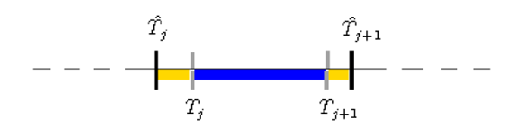
Figure 1: The figure illustrates where we expect to estimate a neighborhood of a node consistently. The blue region corresponds to the overlap between the true block (bounded by gray lines) and the estimated block (bounded by black lines). If the blue region is much larger than the orange regions, the additional bias introduced from the samples from the orange region will not considerably affect the estimation of the neighborhood of a node on the blue region. However, we cannot hope to consistently estimate the neighborhood of a node on the orange region.

Suppose that we know that there is a solution to the optimization problem (3) with the partition boundary $\hat{\mathcal{T}}$. Then that solution is also a minimizer of the following objective

$$\min_{\bm{\theta}^{1},\ldots,\bm{\theta}^{\hat{B}}}\ \ \sum_{j\in\hat{B}}||\mathbf{X}_{a}^{\hat{\mathcal{B}}^{j}}-\mathbf{X}_{\backslash a}^{\hat{\mathcal{B}}^{j}}\bm{\theta}^{j}||_{2}^{2}+2\lambda_{1}\sum_{j=2}^{\hat{B}}||\bm{\theta}^{j}-\bm{\theta}^{j-1}||_{2}+2\lambda_{2}\sum_{j=1}^{\hat{B}}|\hat{\mathcal{B}}^{j}|||\bm{\theta}^{j}||_{1}.$$ (17)

Note that the problem (17) does not give a practical way of solving (3), but will help us to reason about the solutions of (3). In particular, while there may be multiple solutions to the problem (3), under some conditions, we can characterize the sparsity pattern of any solution that has specified partition boundaries $\hat{\mathcal{T}}$.

Lemma 4.

Let $\hat{\bm{\beta}}$ be a solution to (3), with $\hat{\mathcal{T}}$ being an associated estimate of the partition boundaries. Suppose that the subgradient vectors satisfy $|\hat{y}_{i,b}|<1$ for all $b\not\in S(\hat{\bm{\beta}}_{\cdot,i})$, then any other solution $\tilde{\bm{\beta}}$ with the partition boundaries $\hat{\mathcal{T}}$ satisfy $\tilde{\beta}_{b,i}=0$ for all $b\not\in S(\hat{\bm{\beta}}_{\cdot,i})$.

The above Lemma states sufficient conditions under which the sparsity patter of a solution with the partition boundary $\hat{\mathcal{T}}$ is unique. Note, however, that there may other solutions to (3) that have different partition boundaries.

Now, we are ready to state the following theorem, which establishes that the correct neighborhood is selected on every sufficiently large estimated block of the partition.

Theorem 5.

Let $\{\mathbf{x}_{i}\}_{i\in[n]}$ be a sequence of observation according to the model in (1). Assume that the conditions of theorem 2 are satisfied. In addition, suppose that A4 also holds. Then, if $|\hat{\mathcal{T}}|=B+1$, it holds that

$$\mathbb{P}[S^{k}=S(\hat{\bm{\theta}}^{k})]\xrightarrow{n\rightarrow\infty}1,\qquad\forall k\in[B].$$

Under the assumptions of theorem 2 each estimated block is of size $\mathcal{O}(n)$. As a result, there are enough samples in each block to consistently estimate the underlying neighborhood structure. Observe that the neighborhood is consistently estimated at each $i\in\hat{\mathcal{B}}^{j}\cap\mathcal{B}^{j}$ for all $j\in[B]$ and the error is made only on the small fraction of samples, when $i\not\in\hat{\mathcal{B}}^{j}\cap\mathcal{B}^{j}$, which is of order $\mathcal{O}(n\delta_{n})$.

Using proposition 3 in place of theorem 2, it can be similarly shown that, for a large fraction of samples, the neighborhood is consistently estimated even in the case of over-segmentation. In particular, whenever there is a sufficiently large estimated block, with $|\hat{\mathcal{B}}^{k}\cap\mathcal{B}^{j}|=\mathcal{O}(r_{n})$, it holds that $S(\hat{\mathcal{B}}^{k})=S^{j}$ with probability tending to one.

4 Numerical studies

In this section, we present a small numerical study on the proposed algorithm on simulated networks. A full performance test and application on real world data is beyond the scope of this paper which mainly focuses on the theory of time-varying model estimation. In all of our simulations studies we set $p=30$ and $B=3$ with $|\mathcal{B}_{1}|=80$, $|\mathcal{B}_{2}|=130$ and $|\mathcal{B}_{3}|=90$, so that in total we have $n=300$ samples. We consider two types of random networks: a chain and a nearest neighbor network. We measure the performance of the estimation procedure outlined in $\S$2 on the following metrics: average precision of estimated edges, average recall of estimated edges and average $F_{1}$ score which combines the precision and recall score. The precision, recall and $F_{1}$ score are respectively defined as

$$precision =\frac{1}{n}\sum_{i\in[n]}\frac{\sum_{a\in[p]}\sum_{b=a+1}^{p}\operatorname*{1{\hskip-2.5pt}\hbox{I}}\{(a,b)\in\hat{E}_{i}\ \wedge(a,b)\in E_{i}\}}{\sum_{a\in[p]}\sum_{b=a+1}^{p}\operatorname*{1{\hskip-2.5pt}\hbox{I}}\{(a,b)\in\hat{E}_{i}\}}$$

$$recall =\frac{1}{n}\sum_{i\in[n]}\frac{\sum_{a\in[p]}\sum_{b=a+1}^{p}\operatorname*{1{\hskip-2.5pt}\hbox{I}}\{(a,b)\in\hat{E}_{i}\ \wedge(a,b)\in E_{i}\}}{\sum_{a\in[p]}\sum_{b=a+1}^{p}\operatorname*{1{\hskip-2.5pt}\hbox{I}}\{(a,b)\in E_{i}\}}$$

$$F_{1} =\frac{2*precision*recall}{precision+recall}.$$

Our results are averaged over 50 simulation runs. We compare our algorithm against an oracle algorithm which exactly knows the true partition boundaries. In this case, it is only needed to run the algorithm of Meinshausen and Bühlmann (2006) on each block of the partition independently. We use a BIC criterion to select the tuning parameter for this oracle procedure as described in Peng et al. (2009).

Chain networks. We follow the simulation in Fan et al. (2009) to generate a chain network (see Figure 2). This network corresponds to a tridiagonal precision matrix (after an appropriate permutation of nodes). The network is generated as follows. First, we choose generate a random permutation $\pi$ of $[n]$. Next, the covariance matrix is generated as follows: the element at position $(a,b)$ is chosen as $\sigma_{ab}=\exp(-|t_{\pi(a)}-t_{\pi(b)}|/2)$ where $t_{1}<t_{2}<\ldots<t_{p}$ and $t_{i}-t_{i-1}\sim{\rm Unif}(0.5,1)$ for $i=2,\ldots,p$. This processes is repeated three times to obtain three different covariance matrices, from which we sample $80$, $130$ and $90$ samples respectively.

Figure 2: A chain graph

For illustrative purposes, Figure 3 plots the precision, recall and $F_{1}$ score computed for different values of the penalty parameters $\lambda_{1}$ and $\lambda_{2}$. Table 2 shows the precision, recall and $F_{1}$ score for the parameters chosen using the BIC score described in 2.2. The numbers in parentheses correspond to standard deviation. Due to the fact that there is some error in estimating the partition boundaries, we observe a decrease in performance compared to the oracle procedure that knows the correct position of the partition boundaries.

Table 2: Performance on chain networks

Method name	Precision	Recall	$F_{1}$ score
TD-Lasso	0.84 (0.04)	0.80 (0.04)	0.82 (0.04)
Oracle procedure	0.97 (0.02)	0.89 (0.02)	0.93 (0.02)

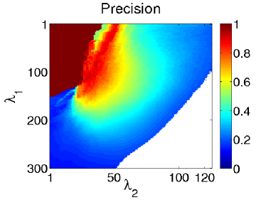
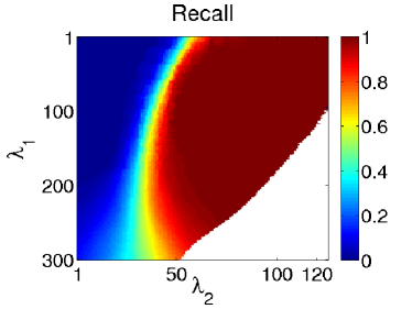
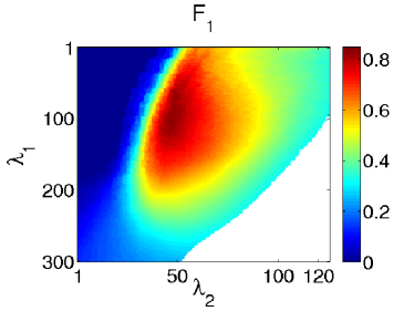
Figure 3: Plots of the precision, recall and $F_{1}$ scores as functions of the penalty parameters $\lambda_{1}$ and $\lambda_{2}$ for chain networks. The parameter $\lambda_{1}$ is obtained as $100*0.98^{50+i}$, where $i$ indexes $y$-axis. The parameter $\lambda_{2}$ is computed as $285*0.98^{230+j}$, where $j$ indexes $x$-axis. The white region of each plot corresponds to a region of the parameter space that we did not explore.

Nearest neighbors networks. We generate nearest neighbor networks following the procedure outlined in Li and Gui (2006). For each node, we draw a point uniformly at random on a unit square and compute the pairwise distances between nodes. Each node is then connected to 4 closest neighbors (see Figure 4). Since some of nodes will have more than 4 adjacent edges, we remove randomly edges from nodes that have degree larger than 4 until the maximum degree of a node in a network is 4. Each edge $(a,b)$ in this network corresponds to a non-zero element in the precision matrix $\bm{\Omega}$, whose value is generated uniformly on $[-1,-0.5]\cup[0.5,1]$. The diagonal elements of the precision matrix are set to a smallest positive number that makes the matrix positive definite. Next, we scale the corresponding covariance matrix $\bm{\Sigma}=\bm{\Omega}^{-1}$ to have diagonal elements equal to 1. This processes is repeated three times to obtain three different covariance matrices, from which we sample $80$, $130$ and $90$ samples respectively.

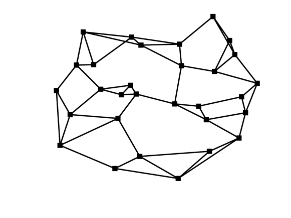
Figure 4: An instance of a random neighborhood graph with 30 nodes.

Table 3: Performance on nearest neighbor networks

Method name	Precision	Recall	$F_{1}$ score
TD-Lasso	0.79 (0.06)	0.76 (0.05)	0.77 (0.05)
Oracle procedure	0.87 (0.05)	0.82 (0.05)	0.84 (0.04)

For illustrative purposes, Figure 5 plots the precision, recall and $F_{1}$ score computed for different values of the penalty parameters $\lambda_{1}$ and $\lambda_{2}$. Table 3 shows the precision, recall and $F_{1}$ score for the parameters chosen using the BIC score, together with their standard deviations. In the same table, we give the results of the oracle procedure.

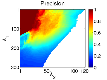
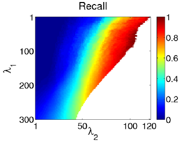
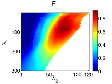
Figure 5: Plots of the precision, recall and $F_{1}$ scores as functions of the penalty parameters $\lambda_{1}$ and $\lambda_{2}$ for nearest neighbor networks. The parameter $\lambda_{1}$ is obtained as $100*0.98^{50+i}$, where $i$ indexes $y$-axis. The parameter $\lambda_{2}$ is computed as $285*0.98^{230+j}$, where $j$ indexes $x$-axis. The white region of each plot corresponds to a region of the parameter space that we did not explore.

5 Conclusion

We have addressed the problem of time-varying covariance selection when the underlying probability distribution changes abruptly at some unknown points in time. Using a penalized neighborhood selection approach with the fused-type penalty, we are able to consistently estimate times when the distribution changes and the network structure underlying the sample. The proof technique used to establish the convergence of the boundary fractions using the fused-type penalty is novel and constitutes an important contribution of the paper. Furthermore, our procedure estimates the network structure consistently whenever there is a large overlap between the estimated blocks and the unknown true blocks of samples coming from the same distribution. The proof technique used to establish the consistency of the network structure builds on the proof for consistency of the neighborhood selection procedure, however, important modifications are necessary since the times of distribution changes are not known in advance. Applications of the proposed approach range from cognitive neuroscience, where the problem is to identify changing associations between different parts of a brain when presented with different stimuli, to system biology studies, where the task is to identify changing patterns of interactions between genes involved in different cellular processes. We conjecture that our estimation procedure is also valid in the high-dimensional setting when the number of variables $p$ is much larger than the sample size $n$. We leave the investigations of the rate of convergence in the high-dimensional setting for a future work.

6 Proofs

6.1 Proof of Lemma 1

For each $i\in[n]$, introduce a $(p-1)$-dimensional vector $\bm{\gamma}_{i}$ defined as

$$\bm{\gamma}_{i}=\left\{\begin{array}[]{ll}\bm{\beta}_{\cdot,i}&\text{for }i=1\\ \bm{\beta}_{\cdot,i}-\bm{\beta}_{\cdot,i-1}&\text{otherwise}\end{array}\right.$$

and rewrite the objective (3) as

$$\{\hat{\bm{\gamma}}^{i}\}_{i\in[n]}=\mathop{\mathrm{argmin}}_{\bm{\gamma}\in\mathbb{R}^{n\times p-1}}\ \sum_{i=1}^{n}(x_{i,a} -\sum_{b\in\backslash a}x_{i,b}\sum_{j\leq i}\gamma_{j,b})^{2}$$ (18)

$$+2\lambda_{1}\sum_{i=2}^{n}||\bm{\gamma}_{i}||_{2}+2\lambda_{2}\sum_{i=1}^{n}\sum_{b\in\backslash a}|\sum_{j\leq i}\gamma_{j,b}|.$$

A necessary and sufficient condition for $\{\hat{\bm{\gamma}}_{i}\}_{i\in[n]}$ to be a solution of (18), is that for each $k\in[n]$ the $(p-1)$-dimensional zero vector, $\mathbf{0}$, belongs to the subdifferential of (18) with respect to $\bm{\gamma}_{k}$ evaluated at $\{\hat{\bm{\gamma}}_{i}\}_{i\in[n]}$, that is,

$$\mathbf{0}=2\sum_{i=k}^{n}(-\mathbf{x}_{i,\backslash a})(x_{i,a}-\sum_{b\in\backslash a}x_{i,b}\hat{\beta}_{b,i}^{a})+2\lambda_{1}\hat{\mathbf{z}}_{k}+2\lambda_{2}\sum_{i=k}^{n}\hat{\mathbf{y}}_{i},$$ (19)

where $\hat{\mathbf{z}}_{k}\in\partial||\cdot||_{2}(\hat{\bm{\gamma}}_{k})$, that is,

$$\tilde{\mathbf{z}}_{k}=\left\{\begin{array}[]{ll}\frac{\tilde{\bm{\gamma}}_{k}}{||\tilde{\bm{\gamma}}_{k}||_{2}}&\text{if }\tilde{\bm{\gamma}}_{k}\neq 0\\ \in\mathcal{B}_{2}(0,1)&\text{otherwise}\end{array}\right.$$

and for $k\leq i$, $\hat{\mathbf{y}}_{i}\in\partial|\sum_{j\leq i}\hat{\bm{\gamma}}_{j}|$, that is, $\mathbf{y}_{i}=\mathop{\mathrm{sign}}(\sum_{j\leq i}\hat{\bm{\gamma}}_{j})$ with $\mathop{\mathrm{sign}}(0)\in[-1,1]$. The Lemma now simply follows from (19).

6.2 Proof of Theorem 2

We build on the ideas presented in the proof of Proposition 5 in Harchaoui and Lévy-Leduc (2010). Using the union bound,

$$\mathbb{P}[\max_{j\in[B]}|T_{j}-\hat{T}_{j}|>n\delta_{n}]\leq\sum_{j\in[B]}\mathbb{P}[|T_{j}-\hat{T}_{j}|>n\delta_{n}]$$

and it is enough to show that $\mathbb{P}[|T_{j}-\tilde{T}_{j}|>n\delta_{n}]\rightarrow 0$ for all $j\in[B]$. Define the event $A_{n,j}$ as

$$A_{n,j}:=\big{\{}|T_{j}-\hat{T}_{j}|>n\delta_{n}\big{\}}$$

and the event $C_{n}$ as

$$C_{n}:=\bigg{\{}\max_{j\in[B]}|\hat{T}_{j}-T_{j}|<\frac{\Delta_{\min}}{2}\bigg{\}}.$$

We show that $\mathbb{P}[A_{n,j}]\rightarrow 0$ by showing that both $\mathbb{P}[A_{n,j}\cap C_{n}]\rightarrow 0$ and $\mathbb{P}[A_{n,j}\cap C_{n}^{c}]\rightarrow 0$ as $n\rightarrow\infty$. The idea here is that, in some sense, the event $C_{n}$ is a good event on which the estimated boundary partitions and the true boundary partitions are not too far from each other. Considering the two cases will make the analysis simpler.

First, we show that $\mathbb{P}[A_{n,j}\cap C_{n}]\rightarrow 0$. Without loss of generality, we assume that $\hat{T}_{j}<T_{j}$, since the other case follows using the same reasoning. Using (15) twice with $k=\hat{T}_{j}$ and with $k=T_{j}$ and then applying the triangle inequality we have

$$2\lambda_{1}\geq\bigg{|}\bigg{|}\sum_{i=\hat{T}_{j}}^{T_{j}-1}\mathbf{x}_{i,\backslash a}\langle{\mathbf{x}_{i,\backslash a}},{\hat{\bm{\beta}}_{\cdot,i}-\bm{\beta}_{\cdot,i}}\rangle-\sum_{i=\hat{T}_{j}}^{\hat{T}_{j}-1}\mathbf{x}_{i,\backslash a}\epsilon_{i}+\lambda_{2}\sum_{i=\hat{T}_{j}}^{T_{j}-1}\hat{\mathbf{y}}_{i}\bigg{|}\bigg{|}_{2}.$$ (20)

Some algebra on the above display gives

$$2\lambda_{1}+(T_{j}-\hat{T}_{j})\sqrt{p}\lambda_{2} \geq\bigg{|}\bigg{|}\sum_{i=\hat{T}_{j}}^{T_{j}-1}\mathbf{x}_{i,\backslash a}\langle\mathbf{x}_{i,\backslash a},\bm{\theta}^{j}-\bm{\theta}^{j+1}\rangle\bigg{|}\bigg{|}_{2}$$

$$\quad-\bigg{|}\bigg{|}\sum_{i=\hat{T}_{j}}^{T_{j}-1}\mathbf{x}_{i,\backslash a}\langle\mathbf{x}_{i,\backslash a},\bm{\theta}^{j+1}-\hat{\bm{\theta}}^{j+1}\rangle\bigg{|}\bigg{|}_{2}-\bigg{|}\bigg{|}\sum_{i=\hat{T}_{j}}^{T_{j}-1}\mathbf{x}_{i,\backslash a}\epsilon_{i}\bigg{|}\bigg{|}_{2}$$

$$=:||R_{1}||_{2}-||R_{2}||_{2}-||R_{3}||_{2}.$$

The above display occurs with probability one, so that the event $\{2\lambda_{1}+(T_{j}-\hat{T}_{j})\sqrt{p}\lambda_{2}\geq\frac{1}{3}||R_{1}||_{2}\}\cup\{||R_{2}||_{2}\geq\frac{1}{3}||R_{1}||_{2}\}\cup\{||R_{3}||_{2}\geq\frac{1}{3}||R_{1}||_{2}\}$ also occurs with probability one, which gives us the following bound

$$\mathbb{P}[A_{n,j}\cap C_{n}] \leq\mathbb{P}[A_{n,j}\cap C_{n}\cap\{2\lambda_{1}+(T_{j}-\hat{T}_{j})\sqrt{p}\lambda_{2}\geq\frac{1}{3}||R_{1}||_{2}\}]$$

$$\quad+\mathbb{P}[A_{n,j}\cap C_{n}\cap\{||R_{2}||_{2}\geq\frac{1}{3}||R_{1}||_{2}\}]$$

$$\quad+\mathbb{P}[A_{n,j}\cap C_{n}\cap\{||R_{3}||_{2}\geq\frac{1}{3}||R_{1}||_{2}\}]$$

$$=:\mathbb{P}[A_{n,j,1}]+\mathbb{P}[A_{n,j,2}]+\mathbb{P}[A_{n,j,3}].$$

First, we focus on the event $A_{n,j,1}$. Using lemma 8, we can upper bound $\mathbb{P}[A_{n,j,1}]$ with

$$\mathbb{P}[2\lambda_{1}+(T_{j}-\hat{T}_{j})\sqrt{p}\lambda_{2}\geq\frac{\phi_{\min}}{27}(T_{j}-\hat{T}_{j})\xi_{\min}]+2\exp(-n\delta_{n}/2+2\log n).$$

Since under the assumptions of the theorem $(n\delta_{n}\xi_{\min})^{-1}\lambda_{1}\rightarrow 0$ and $\xi_{\min}^{-1}\sqrt{p}\lambda_{2}\rightarrow 0$ as $n\rightarrow\infty$, we have that $\mathbb{P}[A_{n,j,1}]\rightarrow 0$ as $n\rightarrow\infty$.

Next, we show that the probability of the event $A_{n,j,2}$ converges to zero. Let $\bar{T}_{j}:=\lfloor 2^{-1}(T_{j}+T_{j+1})\rfloor$. Observe that on the event $C_{n}$, $\hat{T}_{j+1}>\bar{T}_{j}$ so that $\hat{\bm{\beta}}_{\cdot,i}=\hat{\bm{\theta}}^{j+1}$ for all $i\in[T_{j},\bar{T}_{j}]$. Using (15) with $k=T_{j}$ and $k=\bar{T}_{j}$ we have that

$$2\lambda_{1}+(\bar{T}_{j}-T_{j})\sqrt{p}\lambda_{2}\geq\bigg{|}\bigg{|}\sum_{i=T_{j}}^{\bar{T}_{j}-1}\mathbf{x}_{i,\backslash a}\langle{\mathbf{x}_{i,\backslash a}},{\bm{\theta}^{j+1}-\hat{\bm{\theta}}^{j+1}}\rangle\bigg{|}\bigg{|}_{2}-\bigg{|}\bigg{|}\sum_{i=T_{j}}^{\bar{T}_{j}-1}\mathbf{x}_{i,\backslash a}\epsilon_{i}\bigg{|}\bigg{|}_{2}.$$

Using lemma 8 on the display above we have

$$||\bm{\theta}^{j+1}-\hat{\bm{\theta}}^{j+1}||_{2}\leq\frac{36\lambda_{1}+18(\bar{T}_{j}-T_{j})\sqrt{p}\lambda_{2}+18\bigg{|}\bigg{|}\sum_{i=T_{j}}^{\bar{T}_{j}-1}\mathbf{x}_{i,\backslash a}\epsilon_{i}\bigg{|}\bigg{|}_{2}}{(T_{j+1}-T_{j})\phi_{\min}},$$ (21)

which holds with probability at least $1-2\exp(-\Delta_{\min}/4+2\log n)$. We will use the above bound to deal with the event $\{||R_{2}||_{2}\geq\frac{1}{3}||R_{1}||_{2}\}$. Using lemma 8, we have that $\phi_{\min}(T_{j}-\hat{T}_{j})\xi_{\min}/9\leq||R_{1}||_{2}$ and $||R_{2}||_{2}\leq(T_{j}-\hat{T}_{j})9\phi_{\max}||\bm{\theta}^{j+1}-\hat{\bm{\theta}}^{j+1}||_{2}$ with probability at least $1-4\exp(-n\delta_{n}/2+2\log n)$. Combining with (21), the probability $\mathbb{P}[A_{n,j,2}]$ is upper bounded by

$$\mathbb{P} [c_{1}\phi_{\min}^{2}\phi_{\max}^{-1}\Delta_{\min}\xi_{\min}\leq\lambda_{1}]+\mathbb{P}[c_{2}\phi_{\min}^{2}\phi_{\max}^{-1}\xi_{\min}\leq\sqrt{p}\lambda_{2}]+$$

$$\mathbb{P}[c_{3}\phi_{\min}^{2}\phi_{\max}^{-1}\xi_{\min}\leq(\bar{T}_{j}-T_{j})^{-1}||\sum_{i=T_{j}}^{\bar{T}_{j}-1}\mathbf{x}_{i,\backslash a}\epsilon_{i}||_{2}]+c_{4}\exp(-n\delta_{n}/2+2\log n).$$

Under the conditions of the theorem, the first term above converges to zero, since $\Delta_{\min}>n\delta_{n}$ and $(n\delta_{n}\xi_{\min})^{-1}\lambda_{1}\rightarrow 0$. The second term also converges to zero, since $\xi_{\min}^{-1}\sqrt{p}\lambda_{2}\rightarrow 0$. Using lemma 7, the third term converges to zero with the rate $\exp(-c_{6}\log n)$, since $(\xi_{\min}\sqrt{\Delta_{\min}})^{-1}\sqrt{p\log n}\rightarrow 0$. Combining all the bounds, we have that $\mathbb{P}[A_{n,j,2}]\rightarrow 0$ as $n\rightarrow\infty$.

Finally, we upper bound the probability of the event $A_{n,j,3}$. As before, $\phi_{\min}(T_{j}-\hat{T}_{j})\xi_{\min}/9\leq||R_{1}||_{2}$ with probability at least $1-2\exp(-n\delta_{n}/2+2\log n)$. This gives us an upper bound on $\mathbb{P}[A_{n,j,3}]$ as

$$\mathbb{P}\bigg{[}\frac{\phi_{\min}\xi_{\min}}{27}\leq\frac{||\sum_{i=\hat{T}_{j}}^{T_{j}-1}\mathbf{x}_{i,\backslash a}\epsilon_{i}||_{2}}{T_{j}-\hat{T}_{j}}\bigg{]}+2\exp(-n\delta_{n}/2+2\log n),$$

which, using lemma 7, converges to zero as under the conditions of the theorem $(\xi_{\min}\sqrt{n\delta_{n}})^{-1}\sqrt{p\log n}\rightarrow 0$. Thus we have shown that $\mathbb{P}[A_{n,j,3}]\rightarrow 0$. Since the case when $\hat{T}_{j}>T_{j}$ is shown similarly, we have proved that $\mathbb{P}[A_{n,j}\cap C_{n}]\rightarrow 0$ as $n\rightarrow\infty$.

We proceed to show that $\mathbb{P}[A_{n,j}\cap C_{n}^{c}]\rightarrow 0$ as $n\rightarrow\infty$. Recall that $C_{n}^{c}=\{\max_{j\in[B]}|\hat{T}_{j}-T_{j}|\geq\Delta_{\min}/2\}$. Define the following events

$$D_{n}^{(l)} :=\left\{\exists j\in[B],\ \hat{T}_{j}\leq T_{j-1}\right\}\cap C_{n}^{c},$$

$$D_{n}^{(m)} :=\left\{\forall j\in[B],\ T_{j-1}<\hat{T}_{j}<T_{j+1}\right\}\cap C_{n}^{c},$$

$$D_{n}^{(r)} :=\left\{\exists j\in[B],\ \hat{T}_{j}\geq T_{j+1}\right\}\cap C_{n}^{c}$$

and write $\mathbb{P}[A_{n,j}\cap C_{n}^{c}]=\mathbb{P}[A_{n,j}\cap D_{n}^{(l)}]+\mathbb{P}[A_{n,j}\cap D_{n}^{(m)}]+\mathbb{P}[A_{n,j}\cap D_{n}^{(r)}]$. First, consider the event $A_{n,j}\cap D_{n}^{(m)}$ under the assumption that $\hat{T}_{j}\leq T_{j}$. Due to symmetry, the other case will follow in a similar way. Observe that

$$\mathbb{P}[A_{n,j}\cap D_{n}^{(m)}]$$ (22)

$$\leq\mathbb{P}[A_{n,j}\cap\{(\hat{T}_{j+1}-T_{j})\geq\frac{\Delta_{\min}}{2}\}\cap D_{n}^{(m)}]$$

$$\quad+\mathbb{P}[\{(T_{j+1}-\hat{T}_{j+1})\geq\frac{\Delta_{\min}}{2}\}\cap D_{n}^{(m)}]$$

$$\leq\mathbb{P}[A_{n,j}\cap\{(\hat{T}_{j+1}-T_{j})\geq\frac{\Delta_{\min}}{2}\}\cap D_{n}^{(m)}]$$

$$\quad+\sum_{k=j+1}^{B-1}\mathbb{P}[\{(T_{k}-\hat{T}_{k})\geq\frac{\Delta_{\min}}{2}\}\cap\{(\hat{T}_{k+1}-T_{k})\geq\frac{\Delta_{\min}}{2}\}\cap D_{n}^{(m)}].$$

We bound the first term in (22) and note that the other terms can be bounded in the same way. The following analysis is performed on the event $A_{n,j}\cap\{(\hat{T}_{j+1}-T_{j})\geq\Delta_{\min}/2\}\cap D_{n}^{(m)}$. Using (15) with $k=\hat{T}_{j}$ and $k=T_{j}$, after some algebra (similar to the derivation of (20)) the following holds

$$||\bm{\theta}^{j}-\hat{\bm{\theta}}^{j+1}||_{2}\leq\frac{18\lambda_{1}+9(T_{j}-\hat{T}_{j})\sqrt{p}\lambda_{2}+9||\sum_{i=\hat{T}_{j}}^{T_{j}-1}\mathbf{x}_{i,\backslash a}\epsilon_{i}||}{\phi_{\min}(T_{j}-\hat{T}_{j})},$$

with probability at least $1-2\exp(-n\delta_{n}/2+2\log n)$, where we have used lemma 8. Let $\bar{T}_{j}=\lfloor 2^{-1}(T_{j}+T_{j+1})\rfloor$. Using (15) with $k=\bar{T}_{j}$ and $k=T_{j}$ after some algebra (similar to the derivation of (21)) we obtain the following bound

$$||\bm{\theta}^{j}-\bm{\theta}^{j+1}||_{2}\leq \frac{18\lambda_{1}+9(\bar{T}_{j}-T_{j})\sqrt{p}\lambda_{2}+9||\sum_{i=T_{j}}^{\bar{T}_{j}-1}\mathbf{x}_{i,\backslash a}\epsilon_{i}||_{2}}{\phi_{\min}(\bar{T}_{j}-T_{j})}$$

$$+81\phi_{\max}\phi_{\min}^{-1}||\bm{\theta}^{j}-\hat{\bm{\theta}}^{j+1}||_{2},$$

which holds with probability at least $1-c_{1}\exp(-n\delta_{n}/2+2\log n)$, where we have used lemma 8 twice. Combining the last two displays, we can upper bound the first term in (22) with

$$\mathbb{P} [\xi_{\min}n\delta_{n}\leq c_{1}\lambda_{1}]+\mathbb{P}[\xi_{\min}\leq c_{2}\sqrt{p}\lambda_{2}]$$

$$+\mathbb{P}[\xi_{\min}\sqrt{n\delta_{n}}\leq c_{3}\sqrt{p\log n}]+c_{4}\exp(-c_{5}\log n),$$

where we have used lemma 7 to obtain the third term. Under the conditions of the theorem, all terms converge to zero. Reasoning similar about the other terms in (22), we can conclude that $\mathbb{P}[A_{n,j}\cap D_{n}^{(m)}]\rightarrow 0$ as $n\rightarrow\infty$.

Next, we bound the probability of the event $A_{n,j}\cap D_{n}^{(l)}$, which is upper bounded by

$$\mathbb{P}[D_{n}^{(l)}]\leq\sum_{j=1}^{B}2^{j-1}\mathbb{P}[\max\{l\in[B]:\hat{T}_{l}\leq T_{l-1}\}=j].$$

Observe that

$$\{\max \{l\in[B]:\hat{T}_{l}\leq T_{l-1}\}=j\}$$

$$\subseteq\bigcup_{l=j}^{B}\{T_{j}-\hat{T}_{j}\geq\frac{\Delta_{\min}}{2}\}\cap\{\hat{T}_{j+1}-T_{j}\geq\frac{\Delta_{\min}}{2}\}$$

so that we have

$$\mathbb{P}[D_{n}^{(l)}] \leq 2^{B-1}\sum_{j=1}^{B-1}\sum_{l>j}\mathbb{P}[\{T_{l}-\hat{T}_{l}\geq\frac{\Delta_{\min}}{2}\}\cap\{\hat{T}_{l+1}-T_{l}\geq\frac{\Delta_{\min}}{2}\}].$$

Using the same arguments as those used to bound terms in (22), we have that $\mathbb{P}[D_{n}^{(l)}]\rightarrow 0$ as $n\rightarrow\infty$ under the conditions of the theorem. Similarly, we can show that the term $\mathbb{P}[D_{n}^{(r)}]\rightarrow 0$ as $n\rightarrow\infty$. Thus, we have shown that $\mathbb{P}[A_{n,j}\cap C_{n}^{c}]\rightarrow 0$, which concludes the proof.

6.3 Proof of Lemma 4

Consider $\hat{\mathcal{T}}$ fixed. The lemma is a simple consequence of the duality theory, which states that given the subdifferential $\hat{\mathbf{y}}_{i}$ (which is constant for all $i\in\hat{\mathcal{B}}^{j}$, $\hat{\mathcal{B}}^{j}$ being an estimated block of the partition $\hat{\mathcal{T}}$), all solutions $\{\check{\bm{\beta}}_{\cdot,i}\}_{i\in[n]}$ of (3) need to satisfy the complementary slackness condition $\sum_{b\in\backslash a}\hat{y}_{i,b}\check{\beta}_{b,i}=||\check{\bm{\beta}}_{\cdot,i}||_{1}$, which holds only if $\check{\beta}_{b,i}=0$ for all $b\in\backslash a$ for which $|\hat{y}_{i,b}|<1$.

6.4 Proof of Theorem 5

Since the assumptions of theorem 2 are satisfied, we are going to work on the event

$$\mathcal{E}:=\{\max_{j\in[B]}|\hat{T}_{j}-T_{j}|\leq n\delta_{n}\}.$$

In this case, $|\hat{\mathcal{B}}^{k}|=\mathcal{O}(n)$. For $i\in\hat{\mathcal{B}}^{k}$, we write

$$x_{i,a}=\sum_{b\in S^{j}}x_{i,b}\theta_{b}^{k}+e_{i}+\epsilon_{i}$$ (23)

where $e_{i}=\sum_{b\in S}x_{i,b}(\beta_{b,i}-\theta_{b}^{k})$ is the bias. Observe that $\forall i\in\hat{\mathcal{B}}^{k}\cap\mathcal{B}^{k}$, the bias $e_{i}=0$, while for $i\not\in\hat{\mathcal{B}}^{k}\cap\mathcal{B}^{k}$, the bias $e_{i}$ is normally distributed with variance bounded by $M^{2}\phi_{\max}$ under the assumption A1 and A3.

We proceed to show that $S(\hat{\bm{\theta}}^{k})\subset S^{k}$. Since $\hat{\bm{\theta}}^{k}$ is an optimal solution of (3), it needs to satisfy

$$(\mathbf{X}_{\backslash a}^{\hat{\mathcal{B}}^{k}})^{\prime}\mathbf{X}_{\backslash a}^{\hat{\mathcal{B}}^{k}}(\hat{\bm{\theta}}^{k}-\bm{\theta}^{k}) -(\mathbf{X}_{\backslash a}^{\hat{\mathcal{B}}^{k}})^{\prime}(\mathbf{e}^{\hat{\mathcal{B}}^{k}}+\bm{\epsilon}^{\hat{\mathcal{B}}^{k}})$$ (24)

$$+\lambda_{1}(\hat{\mathbf{z}}_{\hat{T}_{k-1}}-\hat{\mathbf{z}}_{\hat{T}_{k}})+\lambda_{2}|\hat{\mathcal{B}}^{k}|\hat{\mathbf{y}}_{\hat{T}_{k-1}}=0.$$

Now, we will construct the vectors $\check{\bm{\theta}}^{k},\check{\mathbf{z}}_{\hat{T}_{k-1}},\check{\mathbf{z}}_{\hat{T}_{k}}$ and $\check{\mathbf{y}}_{\hat{T}_{k-1}}$ that satisfy (24) and verify that the subdifferential vectors are dual feasible. Consider the following restricted optimization problem

$$\min_{\bm{\theta}^{1},\ldots,\bm{\theta}^{\hat{B}};\ \bm{\theta}_{N^{k}}^{k}=\mathbf{0}} \sum_{j\in[\hat{B}]}||\mathbf{X}_{a}^{\hat{\mathcal{B}}^{j}}-\mathbf{X}_{\backslash a}^{\hat{\mathcal{B}}^{j}}\bm{\theta}^{j}||_{2}^{2}$$ (25)

$$+2\lambda_{1}\sum_{j=2}^{\hat{B}}||\bm{\theta}^{j}-\bm{\theta}^{j-1}||_{2}+2\lambda_{2}\sum_{j=1}^{\hat{B}}|\hat{\mathcal{B}}^{j}|||\bm{\theta}^{j}||_{1},$$

where the vector $\bm{\theta}_{N^{k}}^{k}$ is constrained to be $\mathbf{0}$. Let $\{\check{\bm{\theta}}^{j}\}_{j\in[\hat{B}]}$ be a solution to the restricted optimization problem (25). Set the subgradient vectors as $\check{\mathbf{z}}_{\hat{T}_{k-1}}\in\partial||\check{\bm{\theta}}^{k}-\check{\bm{\theta}}^{k-1}||$, $\check{\mathbf{z}}_{T_{k}}\in\partial||\check{\bm{\theta}}^{k+1}-\check{\bm{\theta}}^{k}||$ and $\check{\mathbf{y}}_{\hat{T}_{k-1},S^{k}}=\mathop{\mathrm{sign}}(\check{\bm{\theta}}_{S^{k}}^{k})$. Solve (24) for $\check{\mathbf{y}}_{\hat{T}_{k-1},N^{k}}$. By construction, the vectors $\check{\bm{\theta}}^{k},\check{\mathbf{z}}_{\hat{T}_{k-1}},\check{\mathbf{z}}_{\hat{T}_{k}}$ and $\check{\mathbf{y}}_{\hat{T}_{k-1}}$ satisfy (24). Furthermore, the vectors $\check{\mathbf{z}}_{\hat{T}_{k-1}}$ and $\check{\mathbf{z}}_{\hat{T}_{k}}$ are elements of the subdifferential, and hence dual feasible. To show that $\check{\bm{\theta}}^{k}$ is also a solution to (17), we need to show that $||\check{\mathbf{y}}_{\hat{T}_{k-1},N^{k}}||_{\infty}\leq 1$, that is, that $\check{\mathbf{y}}^{\hat{T}_{k-1}}$ is also dual feasible variable. Using lemma 4, if we show that $\check{\mathbf{y}}_{\hat{T}_{k-1},N^{k}}$ is strict dual feasible, $||\check{\mathbf{y}}_{\hat{T}_{k-1},N^{k}}||_{\infty}<1$, then any other solution $\hat{\check{\bm{\theta}}}^{k}$ to (17) will satisfy $\hat{\check{\bm{\theta}}}_{N}^{k}=\mathbf{0}$.

From (24) we can obtain an explicit formula for $\check{\bm{\theta}}_{S^{k}}$

$$\check{\bm{\theta}}_{S^{k}}^{k}=\bm{\theta}_{S^{k}}^{k} +\left((\mathbf{X}_{S^{k}}^{\hat{\mathcal{B}}^{k}})^{\prime}\mathbf{X}_{S^{k}}^{\hat{\mathcal{B}}^{k}}\right)^{-1}(\mathbf{X}_{S^{k}}^{\hat{\mathcal{B}}})^{\prime}(\mathbf{e}^{\hat{\mathcal{B}}^{k}}+\bm{\epsilon}^{\hat{\mathcal{B}}^{k}})$$ (26)

$$-\left((\mathbf{X}_{S^{k}}^{\hat{\mathcal{B}}^{k}})^{\prime}\mathbf{X}_{S^{k}}^{\hat{\mathcal{B}}^{k}}\right)^{-1}\left(\lambda_{1}(\check{\mathbf{z}}_{\hat{T}_{k-1},S^{k}}-\check{\mathbf{z}}_{\hat{T}_{k},S^{k}})+\lambda_{2}|\hat{\mathcal{B}}^{k}|\check{\mathbf{y}}_{\hat{T}_{k-1},S^{k}}\right).$$

Recall that for large enough $n$ we have that $|\hat{\mathcal{B}}|>p$, so that the matrix $(\mathbf{X}_{S^{k}}^{\hat{\mathcal{B}}^{k}})^{\prime}\mathbf{X}_{S^{k}}^{\hat{\mathcal{B}}^{k}}$ is invertible with probability one. Plugging (26) into (24), we have that $||\check{\mathbf{y}}_{\hat{T}_{k-1},N^{k}}||_{\infty}<1$ if $\max_{b\in N^{k}}|Y_{b}|<1$, where $Y_{b}$ is defined to be

$$Y_{b}:=\left(\mathbf{X}_{b}^{\hat{\mathcal{B}}^{k}}\right)^{\prime}\bigg{[}\mathbf{X}_{S^{k}}^{\hat{\mathcal{B}}^{k}} \left((\mathbf{X}_{S^{k}}^{\hat{\mathcal{B}}^{k}})^{\prime}\mathbf{X}_{S^{k}}^{\hat{\mathcal{B}}^{k}}\right)^{-1}\Big{(}\check{\mathbf{y}}_{\hat{T}_{k-1},S^{k}}+\frac{\lambda_{1}(\hat{\mathbf{z}}_{\hat{T}_{k-1},S^{k}}-\hat{\mathbf{z}}_{\hat{T}_{k},S^{k}})}{|\hat{\mathcal{B}}^{k}|\lambda_{2}}\Big{)}$$ (27)

$$+\mathbf{H}_{S^{k}}^{\hat{\mathcal{B}}^{k},\perp}\Big{(}\frac{\mathbf{e}^{\hat{\mathcal{B}}^{k}}+\bm{\epsilon}^{\hat{\mathcal{B}}^{k}}}{|\hat{\mathcal{B}}^{k}|\lambda_{2}}\Big{)}\bigg{]}-\frac{\lambda_{1}(\check{z}_{\hat{T}_{k-1},b}-\check{z}_{\hat{T}_{k},b})}{|\hat{\mathcal{B}}^{k}|\lambda_{2}},$$

where $\mathbf{H}_{S^{k}}^{\hat{\mathcal{B}}^{k},\perp}$ is the projection matrix

$$\mathbf{H}_{S^{k}}^{\hat{\mathcal{B}}^{k},\perp}=\mathbf{I}-\mathbf{X}_{S^{k}}^{\hat{\mathcal{B}}^{k}}\left((\mathbf{X}_{S^{k}}^{\hat{\mathcal{B}}^{k}})^{\prime}\mathbf{X}_{S^{k}}^{\hat{\mathcal{B}}^{k}}\right)^{-1}\left(\mathbf{X}_{S^{k}}^{\hat{\mathcal{B}}^{k}}\right)^{\prime}.$$

Let $\tilde{\bm{\Sigma}}^{k}$ and $\hat{\tilde{\bm{\Sigma}}}^{k}$ be defined as

$$\tilde{\bm{\Sigma}}^{k}=\frac{1}{|\hat{\mathcal{B}}^{k}|}\sum_{i\in\hat{\mathcal{B}}^{k}}\mathbb{E}[\mathbf{x}_{\backslash a}^{i}(\mathbf{x}_{\backslash a}^{i})^{\prime}]\quad\text{and}\quad\hat{\tilde{\bm{\Sigma}}}^{k}=\frac{1}{|\hat{\mathcal{B}}^{k}|}\sum_{i\in\hat{\mathcal{B}}^{k}}\mathbf{x}_{\backslash a}^{i}(\mathbf{x}_{\backslash a}^{i})^{\prime}.$$

For $i\in[n]$, we let $\mathcal{B}(i)$ index the block to which the sample $i$ belongs to. Now, for any $b\in N^{k}$, we can write $x_{b}^{i}=\bm{\Sigma}_{bS^{k}}^{\mathcal{B}(i)}\big{(}\bm{\Sigma}_{S^{k}S^{k}}^{\mathcal{B}(i)}\big{)}^{-1}\mathbf{x}_{S^{k}}^{i}+w_{b}^{i}$ where $w_{b}^{i}$ is normally distributed with variance $\sigma_{b}^{2}<1$ and independent of $\mathbf{x}_{S^{k}}^{i}$. Let $\mathbf{F}_{b}\in\mathbb{R}^{|\hat{\mathcal{B}}^{k}|}$ be the vector whose components are equal to $\bm{\Sigma}_{bS^{k}}^{\mathcal{B}(i)}\big{(}\bm{\Sigma}_{S^{k}S^{k}}^{\mathcal{B}(i)}\big{)}^{-1}\mathbf{x}_{S^{k}}^{i}$, $i\in\hat{\mathcal{B}}^{k}$, and $\mathbf{W}_{b}\in\mathbb{R}^{|\hat{\mathcal{B}}^{k}|}$ be the vector with components equal to $w_{b}^{i}$. Using this notation, we write $Y_{b}=T_{b}^{1}+T_{b}^{2}+T_{b}^{3}+T_{b}^{4}$ where

$$T_{b}^{1}=\mathbf{F}_{b}^{\prime}\mathbf{X}_{S^{k}}^{\hat{\mathcal{B}}^{k}}\left((\mathbf{X}_{S^{k}}^{\hat{\mathcal{B}}^{k}})^{\prime}\mathbf{X}_{S^{k}}^{\hat{\mathcal{B}}^{k}}\right)^{-1}\Big{(}\check{\mathbf{y}}_{\hat{T}_{k-1}}+\frac{\lambda_{1}(\check{\mathbf{z}}_{\hat{T}_{k-1},S^{k}}-\check{\mathbf{z}}_{\hat{T}_{k},S^{k}})}{|\hat{\mathcal{B}}^{k}|\lambda_{2}}\Big{)}$$ (28)

$$T_{b}^{2}=\mathbf{F}_{b}^{\prime}\mathbf{H}_{S^{k}}^{\hat{\mathcal{B}}^{k},\perp}\Big{(}\frac{\mathbf{e}^{\hat{\mathcal{B}}^{k}}+\bm{\epsilon}^{\hat{\mathcal{B}}^{k}}}{|\hat{\mathcal{B}}^{k}|\lambda_{2}}\Big{)}$$ (29)

$$T_{b}^{3}=\left(\tilde{\mathbf{W}}_{b}\right)^{\prime}\bigg{[}\mathbf{X}_{S^{k}}^{\hat{\mathcal{B}}^{k}} \left((\mathbf{X}_{S^{k}}^{\hat{\mathcal{B}}^{k}})^{\prime}\mathbf{X}_{S^{k}}^{\hat{\mathcal{B}}^{k}}\right)^{-1}\Big{(}\check{\mathbf{y}}_{\hat{T}_{k-1}}+\frac{\lambda_{1}(\check{\mathbf{z}}_{\hat{T}_{k-1},S^{k}}-\check{\mathbf{z}}_{\hat{T}_{k},S^{k}})}{|\hat{\mathcal{B}}^{k}|\lambda_{2}}\Big{)}$$ (30)

$$+\mathbf{H}_{S^{k}}^{\hat{\mathcal{B}}^{k},\perp}\Big{(}\frac{\mathbf{e}^{\hat{\mathcal{B}}^{k}}+\bm{\epsilon}^{\hat{\mathcal{B}}^{k}}}{|\hat{\mathcal{B}}^{k}|\lambda_{2}}\Big{)}\bigg{]}$$

and

$$T_{b}^{4}=-\frac{\lambda_{1}(\check{z}_{\hat{T}_{k-1},b}-\check{z}_{\hat{T}_{k},b})}{|\hat{\mathcal{B}}^{k}|\lambda_{2}}.$$ (31)

We analyze each of the terms separately. Starting with the term $T_{b}^{1}$, after some algebra, we obtain that

$$\mathbf{F}_{b}^{\prime} \mathbf{X}_{S^{k}}^{\hat{\mathcal{B}}^{k}}\left((\mathbf{X}_{S^{k}}^{\hat{\mathcal{B}}^{k}})^{\prime}\mathbf{X}_{S^{k}}^{\hat{\mathcal{B}}^{k}}\right)^{-1}$$ (32)

$$=\sum_{j\ :\ \hat{\mathcal{B}}^{k}\cap\mathcal{B}^{j}\neq\emptyset}\frac{|\mathcal{B}^{j}\cap\hat{\mathcal{B}}^{k}|}{|\hat{\mathcal{B}}^{k}|}\bm{\Sigma}_{bS^{k}}^{j}(\bm{\Sigma}_{S^{k}S^{k}}^{j})^{-1}(\hat{\bm{\Sigma}}_{S^{k}S^{k}}^{\mathcal{B}^{j}\cap\hat{\mathcal{B}}^{k}}-\bm{\Sigma}_{S^{k}S^{k}}^{j})\left({\hat{\tilde{\bm{\Sigma}}}}_{S^{k}S^{k}}^{k}\right)^{-1}$$

$$\quad+\tilde{\bm{\Sigma}}_{bS^{k}}^{k}(({\hat{\tilde{\bm{\Sigma}}}}_{S^{k}S^{k}}^{k})^{-1}-({\tilde{\bm{\Sigma}}_{S^{k}S^{k}}}^{k})^{-1})$$

$$\quad+\tilde{\bm{\Sigma}}_{bS^{k}}^{k}{(\tilde{\bm{\Sigma}}_{S^{k}S^{k}}^{k})}^{-1}.$$

Recall that we are working on the event $\mathcal{E}$, so that $|\!|\!|\tilde{\bm{\Sigma}}_{N^{k}S^{k}}^{k}{(\tilde{\bm{\Sigma}}_{S^{k}S^{k}}^{k})}^{-1}|\!|\!|_{{\infty}}\xrightarrow{n\rightarrow\infty}|\!|\!|\bm{\Sigma}_{N^{k}S^{k}}^{k}{(\bm{\Sigma}_{S^{k}S^{k}}^{k})}^{-1}|\!|\!|_{{\infty}}$ and $(|\hat{\mathcal{B}}^{k}|\lambda_{2})^{-1}\lambda_{1}(\check{\mathbf{z}}_{\hat{T}_{k-1},S^{k}}-\check{\mathbf{z}}_{\hat{T}_{k},S^{k}})\xrightarrow{n\rightarrow\infty}0$ element-wise. Using (37) we bound the first two terms in the equation above. We bound the first term by observing that for any $j$ and any $b\in N^{k}$ and $n$ sufficiently large

$$\frac{|\mathcal{B}^{j}\cap\hat{\mathcal{B}}^{k}|}{|\hat{\mathcal{B}}^{k}|} ||\bm{\Sigma}_{bS^{k}}^{j}(\bm{\Sigma}_{S^{k}S^{k}}^{j})^{-1}(\hat{\bm{\Sigma}}_{S^{k}S^{k}}^{\mathcal{B}^{j}\cap\hat{\mathcal{B}}^{k}}-\bm{\Sigma}_{S^{k}S^{k}}^{j})||_{\infty}$$

$$\leq\frac{|\mathcal{B}^{j}\cap\hat{\mathcal{B}}^{k}|}{|\hat{\mathcal{B}}^{k}|}||\bm{\Sigma}_{bS^{k}}^{j}(\bm{\Sigma}_{S^{k}S^{k}}^{j})^{-1}||_{1}||\hat{\bm{\Sigma}}_{S^{k}S^{k}}^{\mathcal{B}^{j}\cap\hat{\mathcal{B}}^{k}}-\bm{\Sigma}_{S^{k}S^{k}}^{j}||_{\infty}$$

$$\leq C_{1}\frac{|\mathcal{B}^{j}\cap\hat{\mathcal{B}}^{k}|}{|\hat{\mathcal{B}}^{k}|}||\hat{\bm{\Sigma}}_{S^{k}S^{k}}^{\mathcal{B}^{j}\cap\hat{\mathcal{B}}^{k}}-\bm{\Sigma}_{S^{k}S^{k}}^{j}||_{\infty}\leq\epsilon_{1}$$

with probability $1-c_{1}\exp(-c_{2}\log n)$. Next, for any $b\in N^{k}$ we bound the second term as

$$||\tilde{\bm{\Sigma}}_{bS^{k}}^{k}(({\hat{\tilde{\bm{\Sigma}}}}_{S^{k}S^{k}}^{k})^{-1}-({\tilde{\bm{\Sigma}}_{S^{k}S^{k}}}^{k})^{-1})||_{1}$$

$$\quad\leq C_{2}||({\hat{\tilde{\bm{\Sigma}}}}_{S^{k}S^{k}}^{k})^{-1}-({\tilde{\bm{\Sigma}}_{S^{k}S^{k}}}^{k})^{-1})||_{F}$$

$$\quad\leq C_{2}||\tilde{\bm{\Sigma}}_{S^{k}S^{k}}^{k}||_{F}^{2}||\hat{\tilde{\bm{\Sigma}}}_{S^{k}S^{k}}^{k}-\tilde{\bm{\Sigma}}_{S^{k}S^{k}}^{k}||_{F}+\mathcal{O}(||\hat{\tilde{\bm{\Sigma}}}_{S^{k}S^{k}}^{k}-{\tilde{\bm{\Sigma}}_{S^{k}S^{k}}}^{k}||_{F}^{2})$$

$$\leq\epsilon_{2}$$

with probability $1-c_{1}\exp(-c_{2}\log n)$. Choosing $\epsilon_{1},\epsilon_{2}$ sufficiently small and for $n$ large enough, we have that $\max_{b}|T_{b}^{1}|\leq 1-\alpha+o_{p}(1)$ under the assumption A4.

We proceed with the term $T_{b}^{2}$, which can be written as

$$T_{b}^{2} =(|\hat{\mathcal{B}}^{k}|\lambda_{2})^{-1}\left(\bm{\Sigma}_{bS^{k}}^{k}\left(\bm{\Sigma}_{S^{k}S^{k}}^{k}\right)^{-1}-\mathbf{F}_{b}^{\prime}\mathbf{X}_{S^{k}}^{\hat{\mathcal{B}}^{k}}\left((\mathbf{X}_{S^{k}}^{\hat{\mathcal{B}}^{k}})^{\prime}\mathbf{X}_{S^{k}}^{\hat{\mathcal{B}}^{k}}\right)^{-1}\right)\sum_{i\in\mathcal{B}^{k}\cap\hat{\mathcal{B}}^{k}}\mathbf{x}_{S^{k}}^{i}\epsilon^{i}$$

$$+(|\hat{\mathcal{B}}^{k}|\lambda_{2})^{-1}\sum_{i\not\in\mathcal{B}^{k}\cap\hat{\mathcal{B}}^{k}}\left(\bm{\Sigma}_{bS^{k}}^{\mathcal{B}(i)}\left(\bm{\Sigma}_{S^{k}S^{k}}^{\mathcal{B}(i)}\right)^{-1}-\mathbf{F}_{b}^{\prime}\mathbf{X}_{S^{k}}^{\hat{\mathcal{B}}^{k}}\left((\mathbf{X}_{S^{k}}^{\hat{\mathcal{B}}^{k}})^{\prime}\mathbf{X}_{S^{k}}^{\hat{\mathcal{B}}^{k}}\right)^{-1}\right)\mathbf{x}_{S^{k}}^{i}(e^{i}+\epsilon^{i}).$$

Since we are working on the event $\mathcal{E}$ the second term in the above equation is dominated by the first term. Next, using (32) together with (37), we have that for all $b\in N^{k}$

$$||\bm{\Sigma}_{bS^{k}}^{k}\left(\bm{\Sigma}_{S^{k}S^{k}}^{k}\right)^{-1}-\mathbf{F}_{b}^{\prime}\mathbf{X}_{S^{k}}^{\hat{\mathcal{B}}^{k}}\left((\mathbf{X}_{S^{k}}^{\hat{\mathcal{B}}^{k}})^{\prime}\mathbf{X}_{S^{k}}^{\hat{\mathcal{B}}^{k}}\right)^{-1}||_{2}=o_{p}(1).$$

Combining with Lemma 7, we have that under the assumptions of the theorem

$$\max_{b}|T_{b}^{2}|=o_{p}(1).$$

We deal with the term $T_{b}^{3}$ by conditioning on $\mathbf{X}_{S^{k}}^{\hat{\mathcal{B}}^{k}}$ and $\bm{\epsilon}^{\hat{\mathcal{B}}^{k}}$, we have that $\mathbf{W}_{b}$ is independent of the terms in the squared bracket in $T_{b}^{3}$, since all $\check{\mathbf{z}}_{\hat{T}_{k-1},S},\check{\mathbf{z}}_{\hat{T}_{k},S}$ and $\hat{\mathbf{y}}_{\hat{T}_{k-1},S}$ are determined from the solution to the restricted optimization problem. To bound the second term, we observe that conditional on $\mathbf{X}_{S^{k}}^{\hat{\mathcal{B}}^{k}}$ and $\bm{\epsilon}^{\hat{\mathcal{B}}^{k}}$, the variance of $T_{b}^{3}$ can be bounded as

$$\operatorname*{{\rm Var}}(T_{b}^{3}) \leq||\mathbf{X}_{S^{k}}^{\hat{\mathcal{B}}^{k}}\left((\mathbf{X}_{S^{k}}^{\hat{\mathcal{B}}^{k}})^{\prime}\mathbf{X}_{S^{k}}^{\hat{\mathcal{B}}^{k}}\right)^{-1}\check{\eta}_{S^{k}}+\mathbf{H}_{S^{k}}^{\hat{\mathcal{B}}^{k},\perp}\Big{(}\frac{\mathbf{e}^{\hat{\mathcal{B}}^{k}}+\bm{\epsilon}^{\hat{\mathcal{B}}^{k}}}{|\hat{\mathcal{B}}^{k}|\lambda_{2}}\Big{)}||_{2}^{2}$$ (33)

$$\leq\check{\eta}_{S^{k}}^{\prime}\left((\mathbf{X}_{S^{k}}^{\hat{\mathcal{B}}^{k}})^{\prime}\mathbf{X}_{S^{k}}^{\hat{\mathcal{B}}^{k}}\right)^{-1}\check{\eta}_{S^{k}}+\Big{\|}\frac{\mathbf{e}^{\hat{\mathcal{B}}^{k}}+\bm{\epsilon}^{\hat{\mathcal{B}}^{k}}}{|\hat{\mathcal{B}}^{k}|\lambda_{2}}\Big{\|}_{2}^{2},$$

where

$$\check{\eta}_{S^{k}}=\Big{(}\check{\mathbf{y}}_{\hat{T}_{k-1},S^{k}}+\frac{\lambda_{1}(\check{\mathbf{z}}_{\hat{T}_{k-1},S^{k}}-\check{\mathbf{z}}_{\hat{T}_{k},S})}{|\hat{\mathcal{B}}|\lambda_{2}}\Big{)}.$$

Using lemma 8 and Young’s inequality, the first term in (33) is upper bounded by

$$\frac{18}{|\hat{\mathcal{B}}|\phi_{\min}}\left(s+\frac{2\lambda_{1}^{2}}{|\hat{\mathcal{B}}|^{2}\lambda_{2}^{2}}\right)$$

with probability at least $1-2\exp(-|\hat{\mathcal{B}}^{k}|/2+2\log n)$. Using lemma 6 we have that the second term is upper bounded by

$$\frac{(1+\delta^{\prime})(1+M^{2}\phi_{\max})}{|\hat{\mathcal{B}}|\lambda_{2}^{2}}$$

with probability at least $1-\exp(-c_{1}|\hat{\mathcal{B}}^{k}|\delta^{\prime 2}+2\log n)$. Combining the two bounds, we have that $\operatorname*{{\rm Var}}(T_{b}^{3})\leq c_{1}s(|\hat{\mathcal{B}}^{k}|)^{-1}$ with high probability, using the fact that $(|\hat{\mathcal{B}}^{k}|\lambda_{2})^{-1}\lambda_{1}\rightarrow 0$ and $|\hat{\mathcal{B}}^{k}|\lambda_{2}\rightarrow\infty$ as $n\rightarrow\infty$. Using the bound on the variance of the term $T_{b}^{3}$ and the Gaussian tail bound, we have that

$$\max_{b\in N}|T_{b}^{3}|=o_{p}(1).$$

Combining the results, we have that $\max_{b\in N^{k}}|Y_{b}|\leq 1-\alpha+o_{p}(1)$. For a sufficiently large $n$, under the conditions of the theorem, we have shown that $\max_{b\in N}|Y_{b}|<1$ which implies that $\mathbb{P}[S(\hat{\bm{\theta}}^{k})\subset S^{k}]\xrightarrow{n\rightarrow\infty}1$.

Next, we proceed to show that $\mathbb{P}[S^{k}\subset S(\hat{\bm{\theta}}^{k})]\xrightarrow{n\rightarrow\infty}1$. Observe that

$$\mathbb{P}[S^{k}\not\subset S(\hat{\bm{\theta}}^{k})]\leq\mathbb{P}[||\hat{\bm{\theta}}_{S^{k}}^{k}-\bm{\theta}_{S^{k}}^{k}||_{\infty}\geq\theta_{\min}].$$

From (24) we have that $||\hat{\bm{\theta}}_{S^{k}}^{k}-\bm{\theta}_{S^{k}}^{k}||_{\infty}$ is upper bounded by

$$\bigg{|}\bigg{|}\left(\frac{1}{|\hat{\mathcal{B}}^{k}|}(\mathbf{X}_{S^{k}}^{\hat{\mathcal{B}}^{k}})^{\prime}\mathbf{X}_{S^{k}}^{\hat{\mathcal{B}}^{k}}\right)^{-1}\frac{1}{|\hat{\mathcal{B}}^{k}|}(\mathbf{X}_{S^{k}}^{\hat{\mathcal{B}}^{k}})^{\prime}(\tilde{\mathbf{e}}^{\hat{\mathcal{B}}^{k}}+\bm{\epsilon}^{\hat{\mathcal{B}}^{k}})\bigg{|}\bigg{|}_{\infty}$$

$$\qquad\qquad+\bigg{|}\bigg{|}\left((\mathbf{X}_{S^{k}}^{\hat{\mathcal{B}}^{k}})^{\prime}\mathbf{X}_{S^{k}}^{\hat{\mathcal{B}}^{k}}\right)^{-1}\left(\lambda_{1}(\check{\mathbf{z}}_{{\hat{T}_{k-1}},S^{k}}-\check{\mathbf{z}}_{{\hat{T}_{k}},S^{k}})-\lambda_{2}|\hat{\mathcal{B}}^{\hat{\mathcal{B}}^{k}}|\check{\mathbf{y}}_{{\hat{T}_{k-1}},S^{k}}\right)\bigg{|}\bigg{|}_{\infty}.$$

Since $\tilde{e}_{i}\neq 0$ only on $i\in\hat{\mathcal{B}}^{k}\backslash\mathcal{B}^{k}$ and $n\delta_{n}/|\hat{\mathcal{B}}^{k}|\rightarrow 0$, the term involving $\tilde{\mathbf{e}}^{\hat{\mathcal{B}}^{k}}$ is stochastically dominated by the term involving $\bm{\epsilon}^{\hat{\mathcal{B}}^{k}}$ and can be ignored. Define the following terms

$$T_{1} =\left(\frac{1}{|\hat{\mathcal{B}}^{k}|}(\mathbf{X}_{S^{k}}^{\hat{\mathcal{B}}^{k}})^{\prime}\mathbf{X}_{S^{k}}^{\hat{\mathcal{B}}^{k}}\right)^{-1}\frac{1}{|\hat{\mathcal{B}}^{k}|}(\mathbf{X}_{S^{k}}^{\hat{\mathcal{B}}^{k}})^{\prime}\bm{\epsilon}^{\hat{\mathcal{B}}^{k}},$$

$$T_{2} =\left(\frac{1}{|\hat{\mathcal{B}}^{k}|}(\mathbf{X}_{S^{k}}^{\hat{\mathcal{B}}^{k}})^{\prime}\mathbf{X}_{S^{k}}^{\hat{\mathcal{B}}^{k}}\right)^{-1}\frac{\lambda_{1}}{|\hat{\mathcal{B}}^{k}|\lambda_{2}}(\check{\mathbf{z}}_{{\hat{T}_{k-1}},S^{k}}-\check{\mathbf{z}}_{{\hat{T}_{k}},S^{k}}),$$

$$T_{3} =\left(\frac{1}{|\hat{\mathcal{B}}^{k}|}(\mathbf{X}_{S^{k}}^{\hat{\mathcal{B}}^{k}})^{\prime}\mathbf{X}_{S^{k}}^{\hat{\mathcal{B}}^{k}}\right)^{-1}\check{\mathbf{y}}_{{\hat{T}_{k-1}},S^{k}}.$$

Conditioning on $\mathbf{X}_{S^{k}}^{\hat{\mathcal{B}}^{k}}$, the term $T_{1}$ is a $|S^{k}|$ dimensional Gaussian with variance bounded by $c_{1}/n$ with probability at least $1-c_{1}\exp(-c_{2}\log n)$ using lemma 8. Combining with the Gaussian tail bound, the term $||T_{1}||_{\infty}$ can be upper bounded as

$$\mathbb{P}\bigg{[}||T_{1}||_{\infty}\geq c_{1}\sqrt{\frac{\log s}{n}}\bigg{]}\leq c_{2}\exp(-c_{3}\log n).$$ (34)

Using lemma 8, we have that with probability greater than $1-c_{1}\exp(-c_{2}\log n)$

$$||T_{2}||_{\infty}\leq||T_{2}||_{2}\leq c_{3}\frac{\lambda_{1}}{|\hat{\mathcal{B}}^{k}|\lambda_{2}}\rightarrow 0$$

under the conditions of theorem. Similarly $||T_{3}||_{\infty}\leq c_{1}\sqrt{s}$, with probability greater than $1-c_{1}\exp(-c_{2}\log n)$. Combining the terms, we have that

$$||\bm{\theta}^{k}-\hat{\bm{\theta}}^{k}||_{\infty}\leq c_{1}\sqrt{\frac{\log s}{n}}+c_{2}\sqrt{s}\lambda_{2}$$

with probability at least $1-c_{3}\exp(-c_{4}\log n)$. Since $\theta_{\min}=\Omega(\sqrt{\log(n)/n})$, we have shown that $S^{k}\subseteq S(\hat{\bm{\theta}}^{k})$. Combining with the first part, it follows that $S(\hat{\bm{\theta}}^{k})=S^{k}$ with probability tending to one.

Appendix

Technical results

In this section we collect some technical results needed for the proves presented in $\S$6.

Lemma 6.

Let $\{\zeta^{i}\}_{i\in[n]}$ be a sequence of iid $\mathcal{N}(0,1)$ random variables. If $v_{n}\geq C\log n$, for some constant $C>16$, then

$$\mathbb{P}\bigg{[}\bigcap_{{1\leq l<r\leq n}\atop{r-l>r_{n}}}\Big{\{}\sum_{i=l}^{r}(\zeta^{i})^{2}\leq(1+C)(r-l+1)\Big{\}}\bigg{]}\geq 1-\exp(-c_{1}\log n)$$

for some constant $c_{1}>0$.

Proof.

For any $1\leq l<r\leq n$, with $r-l>v_{n}$ we have

$$\mathbb{P}[\sum_{i=l}^{r}(\zeta^{i})^{2}\geq(1+C)(r-l+1)] \leq\exp(-C(r-l+1)/8)$$

$$\leq\exp(-C\log n/8)$$

using (38). The lemma follows from an application of the union bound. ∎

Lemma 7.

Let $\{\mathbf{x}_{i}\}_{i\in[n]}$ be independent observations from (1) and let $\{\epsilon_{i}\}_{i\in[n]}$ be independent $\mathcal{N}(0,1)$. Assume that A1 holds. If $v_{n}\geq C\log n$ for some constant $C>16$, then

$$\mathbb{P}\bigg{[}\bigcap_{j\in[B]} \bigcap_{{l,r\in\mathcal{B}^{j}}\atop{r-l>v_{n}}}\ \bigg{\{}\frac{1}{r-l+1}||\sum_{i=l}^{r}\mathbf{x}_{i}\epsilon_{i}||_{2}\leq\frac{\phi_{\max}^{1/2}\sqrt{1+C}}{\sqrt{r-l+1}}\sqrt{p(1+C\log n)}\Big{\}}\bigg{]}$$

$$\geq 1-c_{1}\exp(-c_{2}\log n),$$

for some constants $c_{1},c_{2}>0$.

Proof.

Let $\bm{\Sigma}^{1/2}$ denote the symmetric square root of the covariance matrix $\bm{\Sigma}_{SS}$ and let $\mathcal{B}(i)$ denote the block $\mathcal{B}^{j}$ of the true partition such that $i\in\mathcal{B}^{j}$. With this notation, we can write $\mathbf{x}_{i}=\left(\bm{\Sigma}^{\mathcal{B}(i)}\right)^{1/2}\mathbf{u}_{i}$ where $\mathbf{u}_{i}\sim\mathcal{N}(\mathbf{0},\mathbf{I})$. For any $l\leq r\in\mathcal{B}^{j}$ we have

$$||\sum_{i=l}^{r}\mathbf{x}_{i}\epsilon_{i}||_{2}=||\sum_{i=l}^{r}\left(\bm{\Sigma}^{j}\right)^{1/2}\mathbf{u}_{i}\epsilon_{i}||_{2}\leq\phi_{\max}^{1/2}||\sum_{i=l}^{r}\mathbf{u}_{i}\epsilon_{i}||_{2}.$$

Conditioning on $\{\epsilon_{i}\}_{i}$, for each $b\in[p]$, $\sum_{i=l}^{r}u_{i,b}\epsilon_{i}$ is a normal random variable with variance $\sum_{i=l}^{r}(\epsilon_{i})^{2}$. Hence, $||\sum_{i=l}^{r}\mathbf{u}_{i}\epsilon_{i}||_{2}^{2}/(\sum_{i=l}^{r}(\epsilon_{i})^{2})$ conditioned on $\{\epsilon_{i}\}_{i}$ is distributed according to $\chi^{2}_{p}$ and

$$\mathbb{P}\bigg{[}\frac{1}{r-l+1} ||\sum_{i=l}^{r}\mathbf{x}_{i}\epsilon_{i}||_{2}\geq\frac{\phi_{\max}^{1/2}\sqrt{\sum_{i=l}^{r}(\epsilon_{i})^{2}}}{r-l+1}\sqrt{p(1+C\log n)}\ \Big{|}\ \{\epsilon_{i}\}_{i=l}^{r}\bigg{]}$$

$$\leq\mathbb{P}[\chi^{2}_{p}\geq p(1+C\log n)]\leq\exp(-C\log n/8),$$

where the last inequality follows from (38). Using lemma 6, for all $l,r\in\mathcal{B}^{j}$ with $r-l>v_{n}$ the quantity $\sum_{i=l}^{r}(\epsilon_{i})^{2}$ is bounded by $(1+C)(r-l+1)$ with probability at least $1-\exp(-c_{1}\log n)$, which gives us the following bound

$$\mathbb{P}\bigg{[}\bigcap_{j\in[B]} \bigcap_{{l,r\in\mathcal{B}^{j}}\atop{r-l>v_{n}}}\ \bigg{\{}\frac{1}{r-l+1}||\sum_{i=l}^{r}\mathbf{x}_{i}\epsilon_{i}||_{2}\leq\frac{\phi_{\max}^{1/2}\sqrt{1+C}}{\sqrt{r-l+1}}\sqrt{p(1+C\log n)}\Big{\}}\bigg{]}$$

$$\geq 1-c_{1}\exp(-c_{2}\log n).$$

∎

Lemma 8.

Let $\{\mathbf{x}_{i}\}_{i\in[n]}$ be independent observations from (1). Assume that A1 holds. Then for any $v_{n}>p$,

$$\mathbb{P}\Big{[}\max_{{1\leq l<r\leq n}\atop{r-l>v_{n}}}\ \Lambda_{\max}\left(\frac{1}{r-l+1}\sum_{i=l}^{r}\mathbf{x}_{i}\left(\mathbf{x}_{i}\right)^{\prime}\right)\geq 9\phi_{\max}\Big{]}\leq 2n^{2}\exp(-v_{n}/2)$$

and

$$\mathbb{P}\Big{[}\min_{{1\leq l<r\leq n}\atop{r-l>v_{n}}}\ \Lambda_{\min}\left(\frac{1}{r-l+1}\sum_{i=l}^{r}\mathbf{x}_{i}\left(\mathbf{x}_{i}\right)^{\prime}\right)\leq\phi_{\min}/9\Big{]}\leq 2n^{2}\exp(-v_{n}/2).$$

Proof.

For any $1\leq l<r\leq n$, with $r-l\geq v_{n}$ we have

$$\mathbb{P}\Big{[}\Lambda_{\max}\left(\frac{1}{r-l+1}\sum_{i=l}^{r}\mathbf{x}_{i}\left(\mathbf{x}_{i}\right)^{\prime}\right)\geq 9\phi_{\max}\Big{]} \leq 2\exp(-(r-l+1)/2)$$

$$\leq 2\exp(-v_{n}/2)$$

using (35), convexity of $\Lambda_{\max}(\cdot)$ and A1. The lemma follows from an application of the union bound. The other inequality follows using a similar argument. ∎

Proof of Proposition 3

The following proof follows main ideas already given in theorem 2. We provide only a sketch.

Given an upper bound on the number of partitions $B_{\max}$, we are going to perform the analysis on the event $\{\hat{B}\leq B_{\max}\}$. Since

$$\mathbb{P}[h(\hat{\mathcal{T}},{\mathcal{T}})\geq n\delta_{n}\ \big{|}\ \{\hat{B}\leq B_{\max}\}]\leq\sum_{B^{\prime}=B}^{B_{\max}}\mathbb{P}[h(\hat{\mathcal{T}},{\mathcal{T}})\geq n\delta_{n}\ \big{|}\ \{|\hat{\mathcal{T}}|=B^{\prime}+1\}],$$

we are going to focus on $\mathbb{P}[h(\hat{\mathcal{T}},{\mathcal{T}})\geq n\delta_{n}\ \big{|}\ \{|\hat{\mathcal{T}}|=B^{\prime}+1\}]$ for $B^{\prime}>B$ (for $B^{\prime}=B$ it follows from theorem 2 that $h(\hat{\mathcal{T}},{\mathcal{T}})<n\delta_{n}$ with high probability). Let us define the following events

$$\mathcal{E}_{j,1} =\{\exists l\in[B^{\prime}]\ :\ |\hat{T}_{l}-T_{j}|\geq n\delta_{n},|\hat{T}_{l+1}-T_{j}|\geq n\delta_{n}\text{ and }\hat{T}_{l}<T_{j}<\hat{T}_{l+1}\}$$

$$\mathcal{E}_{j,2} =\{\forall l\in[B^{\prime}]\ :\ |\hat{T}_{l}-T_{j}|\geq n\delta_{n}\text{ and }\hat{T}_{l}<T_{j}\}$$

$$\mathcal{E}_{j,3} =\{\forall l\in[B^{\prime}]\ :\ |\hat{T}_{l}-T_{j}|\geq n\delta_{n}\text{ and }\hat{T}_{l}>T_{j}\}.$$

Using the above events, we have the following bound

$$\mathbb{P}[h(\hat{\mathcal{T}},{\mathcal{T}})\geq n\delta_{n}\ \big{|}\ \{|\hat{\mathcal{T}}|=B^{\prime}+1\}]\leq\sum_{j\in[B]}\mathbb{P}[\mathcal{E}_{j,1}]+\mathbb{P}[\mathcal{E}_{j,2}]+\mathbb{P}[\mathcal{E}_{j,3}].$$

The probabilities of the above events can be bounded using the same reasoning as in the proof of theorem 2, by repeatedly using the KKT conditions given in (15). In particular, we can use the strategy used to bound the event $A_{n,j,2}$. Since the proof is technical and does not reveal any new insight, we omit the details.

A collection of known results

This section collects some known results that we have used in the paper. We start by collecting some results on the eigenvalues of random matrices. Let $\mathbf{x}\stackrel{{\scriptstyle{iid}}}{{\sim}}\mathcal{N}(0,\bm{\Sigma})$, $i\in[n]$, and $\hat{\bm{\Sigma}}=n^{-1}\sum\mathbf{x}_{i}(\mathbf{x}_{i})^{\prime}$ be the empirical covariance matrix. Denote the elements of the covariance matrix $\bm{\Sigma}$ as $[\sigma_{ab}]$ and of the empirical covariance matrix $\hat{\bm{\Sigma}}$ as $[\hat{\sigma}_{ab}]$.

Using standard results on concentration of spectral norms and eigenvalues (Davidson and Szarek, 2001), Wainwright (2009) derives the following two crude bounds that can be very useful. Under the assumption that $p<n$,

$$\mathbb{P}[\Lambda_{\max}(\hat{\bm{\Sigma}})\geq 9\phi_{\max}] \leq 2\exp(-n/2)$$ (35)

$$\mathbb{P}[\Lambda_{\min}(\hat{\bm{\Sigma}})\leq\phi_{\min}/9] \leq 2\exp(-n/2).$$ (36)

From Lemma A.3. in Bickel and Levina (2008) we have the following bound on the elements of the covariance matrix

$$\mathbb{P}[|\hat{\sigma}_{ab}-\sigma_{ab}|\geq\epsilon]\leq c_{1}\exp(-c_{2}n\epsilon^{2}),\qquad|\epsilon|\leq\epsilon_{0}$$ (37)

where $c_{1}$ and $c_{2}$ are positive constants that depend only on $\Lambda_{\max}(\bm{\Sigma})$ and $\epsilon_{0}$.

Next, we use the following tail bound for $\chi^{2}$ distribution from Lounici et al. (2009), which holds for all $\epsilon>0$,

$$\mathbb{P}[\chi^{2}_{n}>n+\epsilon]\leq\exp(-\frac{1}{8}\min(\epsilon,\frac{\epsilon^{2}}{n})).$$ (38)

References

- Ahmed and Xing (2009) Amr Ahmed and Eric P. Xing. Recovering time-varying networks of dependencies in social and biological studies. Proceedings of the National Academy of Sciences, 106(29):11878–11883, July 2009. doi: 10.1073/pnas.0901910106. URL http://www.pnas.org/content/106/29/11878.abstract.
- Bai and Perron (1998) Jushan Bai and Pierre Perron. Estimating and testing linear models with multiple structural changes. Econometrica, 66(1):47–78, January 1998. URL http://ideas.repec.org/a/ecm/emetrp/v66y1998i1p47-78.html.
- Banerjee et al. (2008) Onureena Banerjee, Laurent El Ghaoui, and Alexandre d’Aspremont. Model selection through sparse maximum likelihood estimation for multivariate gaussian or binary data. J. Mach. Learn. Res., 9:485–516, 2008. ISSN 1533-7928.
- Beck and Teboulle (2009) A. Beck and M. Teboulle. A fast iterative shrinkage-thresholding algorithm for linear inverse problems. SIAM Journal on Imaging Sciences, 2(1):183–202, 2009.
- Bickel and Levina (2008) Peter J. Bickel and Elizaveta Levina. Regularized estimation of large covariance matrices. Annals of Statistics, 36(1):199–227, 2008.
- Boyd and Vandenberghe (2004) Stephen Boyd and Lieven Vandenberghe. Convex Optimization. Cambridge University Press, 2004. ISBN 0521833787.
- Bunea (2008) Florentina Bunea. Honest variable selection in linear and logistic regression models via and penalization. Electronic Journal of Statistics, 2:1153, 2008. URL doi:10.1214/08-EJS287.
- Davidson and Szarek (2001) K.R. Davidson and S.J. Szarek. Local operator theory, random matrices and Banach spaces. Handbook of the geometry of Banach spaces, 1:317–366, 2001.
- Dempster (1972) A. P. Dempster. Covariance selection. Biometrics, 28(1):157–175, 1972. ISSN 0006341X. URL http://www.jstor.org/stable/2528966.
- Fan et al. (2009) Jianqing Fan, Yang Feng, and Yichao Wu. Network exploration via the adaptive LASSO and SCAD penalties. The Annals of Applied Statistics, 3(2):521–541, 2009. doi: 10.1214/08-AOAS215. URL http://projecteuclid.org/DPubS?service=UI&version=1.0&verb=Display&hand%le=euclid.aoas/1245676184.
- Friedman et al. (2008) Jerome Friedman, Trevor Hastie, and Robert Tibshirani. Sparse inverse covariance estimation with the graphical lasso. Biostat, 9(3):432–441, 2008. doi: 10.1093/biostatistics/kxm045. URL http://biostatistics.oxfordjournals.org/cgi/content/abstract/9/3/432.
- Getoor and Taskar (2007) L. Getoor and B. Taskar. Introduction to Statistical Relational Learning (Adaptive Computation and Machine Learning). The MIT Press, August 2007. ISBN 0262072882. URL http://www.amazon.com/exec/obidos/redirect?tag=citeulike07-20&path=ASIN%/0262072882.
- Guo et al. (2010a) J. Guo, E. Levina, G. Michailidis, and J. Zhu. Joint Structure Estimation for Categorical Markov Networks. 2010a.
- Guo et al. (2010b) J. Guo, E. Levina, G. Michailidis, and J. Zhu. Joint Estimation of Multiple Graphical Models. 2010b.
- Harchaoui and Lévy-Leduc (2010) Zaïd Harchaoui and Céline Lévy-Leduc. Multiple change-point estimation with a total-variation penalty. Journal of the American Statistical Association, 105(492), 2010.
- Hastie and Tibshirani (1993) Trevor Hastie and Robert Tibshirani. Varying-coefficient models. Journal of the Royal Statistical Society. Series B (Methodological), 55(4):757–796, 1993. ISSN 00359246. URL http://www.jstor.org/stable/2345993.
- Kolar and Xing (2009) Mladen Kolar and Eric P Xing. Sparsistent estimation of Time-Varying discrete markov random fields. 0907.2337, July 2009. URL http://arxiv.org/abs/0907.2337.
- Kolar et al. (2010a) Mladen Kolar, Ankur P. Parikh, and Eric P. Xing. On sparse nonparametric conditional covariance selection. In ICML ’10: Proceedings of the 27th Annual International Conference on Machine Learning, 2010a.
- Kolar et al. (2010b) Mladen Kolar, Le Song, Amr Ahmed, and Eric P. Xing. Estimating Time-Varying networks. Annals of Applied Statistics, 4(1):94—123, 2010b.
- Lauritzen (1996) S. L. Lauritzen. Graphical Models (Oxford Statistical Science Series). Oxford University Press, USA, July 1996.
- Li and Gui (2006) H. Li and J. Gui. Gradient directed regularization for sparse Gaussian concentration graphs, with applications to inference of genetic networks. Biostatistics, 7(2):302, 2006.
- Liu et al. (1997) J. Liu, S. Wu, and J. V Zidek. On segmented multivariate regression. Statistica Sinica, 7:497–526, 1997.
- Lounici et al. (2009) Karim Lounici, Massimiliano Pontil, Alexandre B. Tsybakov, and Sara van de Geer. Taking advantage of sparsity in Multi-Task learning. In Proceedings of the Conference on Learning Theory (COLT), 2009. URL http://arxiv.org/abs/0903.1468.
- Mammen and van de Geer (1997) Enno Mammen and Sara van de Geer. Locally adaptive regression splines. Annals of Statistics, 25(1):387–413, 1997. ISSN 00905364.
- Meinshausen and Bühlmann (2006) Nicolai Meinshausen and Peter Bühlmann. High-dimensional graphs and variable selection with the lasso. Annals of Statistics, 34(3):1436–1462, 2006.
- Nesterov (2007) Y. Nesterov. Gradient methods for minimizing composite objective function. Center for Operations Research and Econometrics (CORE), Catholic University of Louvain, Tech. Rep, 76:2007, 2007.
- Nesterov (2005) Yu. Nesterov. Smooth minimization of non-smooth functions. Mathematical Programming, 103(1):127–152, May 2005. doi: 10.1007/s10107-004-0552-5. URL http://dx.doi.org/10.1007/s10107-004-0552-5.
- Peng et al. (2009) Jie Peng, Pei Wang, Nengfeng Zhou, and Ji Zhu. Partial correlation estimation by joint sparse regression models. Journal of the American Statistical Association, 104(486):735–746, 2009. doi: 10.1198/jasa.2009.0126. URL http://pubs.amstat.org/doi/abs/10.1198/jasa.2009.0126.
- Ravikumar et al. (2008) P. Ravikumar, M. J. Wainwright, G. Raskutti, and B. Yu. High-dimensional covariance estimation by minimizing -penalized log-determinant divergence. Nov 2008.
- Ravikumar et al. (2009) P. Ravikumar, M. J. Wainwright, and J. D. Lafferty. High-dimensional ising model selection using regularized logistic regression. Annals of Statistics, to appear, 2009.
- Rinaldo (2009) Alessandro Rinaldo. Properties and refinements of the fused lasso. The Annals of Statistics, 37(5):2922–2952, 2009. doi: 10.1214/08-AOS665. URL http://projecteuclid.org/DPubS?service=UI&version=1.0&verb=Display&hand%le=euclid.aos/1247836673.
- Rothman et al. (2008) Adam J. Rothman, Peter J. Bickel, Elizaveta Levina, and Ji Zhu. Sparse permutation invariant covariance estimation. Electronic Journal Of Statistics, 2:494, 2008.
- Tibshirani et al. (2005) Robert Tibshirani, Michael Saunders, Saharon Rosset, Ji Zhu, and Keith Knight. Sparsity and smoothness via the fused lasso. Journal Of The Royal Statistical Society Series B, 67(1):91–108, 2005. URL http://ideas.repec.org/a/bla/jorssb/v67y2005i1p91-108.html.
- van de Geer and Bühlmann (2009) Sara A. van de Geer and Peter Bühlmann. On the conditions used to prove oracle results for the lasso. Electronic Journal of Statistics, 3:1360–1392, 2009. doi: 10.1214/09-EJS506.
- Wainwright (2009) Martin J. Wainwright. Sharp thresholds for high-dimensional and noisy sparsity recovery using -constrained quadratic programming (lasso). IEEE Transactions on Information Theory, 55(5):2183–2202, May 2009. ISSN 0018-9448. doi: 10.1109/TIT.2009.2016018.
- Wainwright and Jordan (2008) Martin J. Wainwright and Michael I. Jordan. Graphical models, exponential families, and variational inference. Found. Trends Mach. Learn., 1(1-2):1–305, 2008. ISSN 1935-8237. doi: 10.1561/2200000001. URL http://dx.doi.org/10.1561/2200000001.
- Wang et al. (2009) Pei Wang, Dennis L Chao, and Li Hsu. Learning networks from high dimensional binary data: An application to genomic instability data. 0908.3882, August 2009. URL http://arxiv.org/abs/0908.3882.
- Yin et al. (2008) Jianxin Yin, Zhi Geng, Runze Li, and Hansheng Wang. Nonparametric Covariance Model. Statistica Sinica, Forthcoming, 2008.
- Yuan and Lin (2007) Ming Yuan and Yi Lin. Model selection and estimation in the gaussian graphical model. Biometrika, 94(1):19–35, March 2007. doi: 10.1093/biomet/asm018. URL http://biomet.oxfordjournals.org/cgi/content/abstract/94/1/19.
- Zhao and Yu (2006) Peng Zhao and Bin Yu. On model selection consistency of lasso. J. Mach. Learn. Res., 7:2541–2563, 2006. ISSN 1533-7928.
- Zhou et al. (2008) Shuheng Zhou, John Lafferty, and Larry Wasserman. Time varying undirected graphs. In Rocco A. Servedio and Tong Zhang, editors, COLT, pages 455–466. Omnipress, 2008.