Radially Extended, Stratified, Local Models of Isothermal Disks

Abstract

We consider local, stratified, numerical models of isothermal accretion disks. The novel feature of our treatment is that radial extent $L_{x}$ and azimuthal extent $L_{y}$ satisfy $H\ll L_{x},L_{y}\ll R$, where $H$ is the scale height and $R$ is the local radius. This enables us to probe mesoscale structure in stratified thin disks. We evolve the model at several resolutions, sizes, and initial magnetic field strengths. Consistent with earlier work, we find that the saturated, turbulent state consists of a weakly magnetized disk midplane coupled to a strongly magnetized corona, with a transition at $|z|\sim 2H$. The saturated $\alpha\simeq 0.01-0.02$. A two-point correlation function analysis reveals that the central $4H$ of the disk is dominated by small scale turbulence that is statistically similar to unstratified disk models, while the coronal magnetic fields are correlated on scales $\sim 10H$. Nevertheless angular momentum transport through the corona is small. A study of magnetic field loops in the corona reveals few open field lines and predominantly toroidal loops with a characteristic distance between footpoints that is $\sim H$. Finally we find quasi-periodic oscillations with characteristic timescale $\sim 30\Omega^{-1}$ in the magnetic field energy density. These oscillations are correlated with oscillations in the mean azimuthal field; we present a phenomenological, alpha-dynamo model that captures most aspects of the oscillations.

1 Introduction

The physics of angular momentum transport is at the core of accretion disk studies. Classical viscous thin disk theories (Shakura & Sunyaev (1973); Lynden-Bell & Pringle (1974); Novikove & Thorne (1973)) assume the existence of a local turbulent viscous stress, thus provide a simple local parameterization, i.e., “anomalous viscosity” $\alpha$, for disk momentum transport and dissipation. Since the early 90’s, the magnetorotational instability (MRI, Balbus & Hawley (1991)) has been regarded as the best candidate to drive accretion disk turbulence, although gravitational torque or magnetic winds of a Blandford & Payne (1982) type can also enhance angular momentum transport.

Classical thin disk theories are vertically integrated and azimuthally averaged, therefore essentially one dimensional. Currently, disk vertical structure can only be obtained from numerical simulations where turbulence is established from first-principle instabilities such as the MRI. Global disk simulations are just starting to investigate thin disks (Reynolds & Fabian (2008); Shafee et al. (2008); Noble et al. (2009)), but they are computationally expensive and not yet able to fully resolve turbulent structures in the disk. Shearing box simulations, on the other hand, can concentrate resolution on disk dynamics at scales of order the disk scale height $H\equiv c_{s}/\Omega$, therefore are more suitable to study accretion flows in detail. Past studies of shearing box simulations with vertical gravity (e.g., Brandenburg et al. (1995); Stone et al. (1996); Miller & Stone (2000); Hirose et al. (2006); Blaes et al. (2007); Suzuki & Inutsuka (2009)) have revealed a rich set of structures and dynamics in stratified disks. However, all these stratified shearing box simulations were done with a box of limited radial extent $L_{x}\sim H$, therefore they were not able to explore any structure on scales larger than $H$. Recently, Davis et al. (2010) have studied stratified shearing box of radial extent $L_{x}=4H$, and Johansen et al. (2009) have adopted models of box size up to $L_{x}\sim 10H$ in their zonal flow studies. However both these studies are limited to the small veritical extent ($\sim\pm 2H$) and physically unrealistic periodic vertical boundary conditions. In this paper we study the dynamics and structure in isothermal stratified disks using large shearing box with domain sizes $L_{x}\geq 10H$ in all directions.

We still do not know whether a magnetized turbulent disk is well modeled as a steady-state, locally dissipated disk model. It is possible, for example, that structures (gas and/or fields) develop at a scale large compared to $H$, and that these structures could be associated with nonlocal energy or angular momentum transport. Large scale structures might also develop in the magnetic field in the form of dynamo. The disk might also be secularly unstable (see the overview by Piran (1978)), that could cause the disk to break up into rings. It is well known that a Navier-Stokes viscosity model for disk turbulence leads, for some opacity regimes, to both viscous (Lightman & Eardley, 1974) and thermal Piran (1978) instability, although it is now believed that thermal instability can be removed by delays imposed through finite relaxation time effects in MRI-driven turbulence (Hirose et al. (2009)).

¿From an observational point of view, the level of fluctuations (inhomogeneity) at different locations in disks and how these different locations communicate with each other have important consequences for disk spectra modeling (Davis et al., 2005; Blaes et al., 2006). In these models observational diagnostics require integrating over the disk surface, so radially extended structure in the disk model may change the disk spectrum. Our disk model is isothermal (we do not solve an energy equation) and is therefore not capable of investigating dissipation and radiation. It is possible that larger fluctuations would appear in physically richer models where thermodynamics and radiative effects are taken into account (e.g., Turner et al. (2003); Turner (2004)). It would then be interesting in the future for spectral modelers to consider disk models with larger radial domains.

A shearing box larger than $H$ is also essential to catch the field structure and dynamics in the accretion disk magnetic coronae (ADC; Tout & Pringle (1996); also see a discussion in Uzdensky & Goodman (2008)), where the field has a characteristic curvature $l\sim v_{a}/\Omega\geq H$, and $v_{a}$ is the characteristic Alfvén speed in the region.

Recently, it has also been pointed out that a large box size may be important to study the saturation properties of the MRI-driven turbulence, either on the ground of resolving parasitic modes (Pessah & Goodman, 2009), or in a phenomenological model of an MRI driven dynamo (Vishniac, 2009). Saturation mechanisms in stratified disk may be fundamentally different from those in unstratified disks. Recent numerical experiments on unstratified disks suggest that: (a) with a zero-net flux, the saturation is dependent on the microscopic Prandtl number ${\rm\,Pr}_{M}$ in the disk, at least at the low Reynolds number (Fromang & Papaloizou, 2007; Lesur & Longaretti, 2007; Simon & Hawley, 2009); (b) with a net (toroidal or vertical) flux, the saturation increases with resolution (Hawley et al., 1995; Guan et al., 2009). Stratified disk models, which are closer to real disks, may well maintain a net (most likely, toroidal; see a discussion in Guan & Gammie (2009)) field in the disk region because of the magnetic buoyancy induced by stratification. Therefore we expect a saturation in stratified disk models to differ from unstratified models.

It is worth enumerating the assumptions we adopt in this work: (1) we use an isothermal equation of state (EOS) in our models; (2) the vertical support comes from the gas and magnetic pressure rather than the radiation pressure; (3) there is no explicit viscosity or resistivity; (4) our initial conditions consist of a uniform toroidal field in a region near the disk midplane; (5) we use outflow boundary conditions for the vertical boundaries.

The paper is organized as follows. In §2 we give a description of the local model and summarize our numerical algorithm. In §3 we present a fiducial model and analyze its structure in the saturated state. In §4 we describe how this structure depends on model parameters. In §5 we give a report on quasiperiodic oscillations (“butterfly diagrams”) and present a phenomenological model to describe them that is based on a mean-field dynamo model; §5 contains a summary of our results.

2 Local Model and Numerical Methods

The local model for disks can be obtained by expanding the equations of motion around a circular-orbiting coordinate origin, with $(r,\phi,z)=(r_{o},\Omega_{o}t+\phi_{o},0)$ in cylindrical coordinates, assuming that the peculiar velocities are comparable to the sound speed and that the sound speed is small compared to the orbital velocity. The local Cartesian coordinates are then obtained from cylindrical coordinates via $(x,y,z)=(r-r_{o},r_{o}[\phi-\Omega_{o}t-\phi_{o}],z)$. In this work we assume the disk sits in a Keplerian ($1/r$) potential. We also use an isothermal ($p=c_{s}^{2}\rho$, where $c_{s}$ is constant) EOS.

For an ideal MHD disk, the equation of motion in the local model is

$$\frac{\partial\mbox{\boldmath$v$}}{\partial t}+\mbox{\boldmath$v$}\cdot\mbox{\boldmath$\nabla$}\mbox{\boldmath$v$}+c_{s}^{2}\frac{\mbox{\boldmath$\nabla$}\rho}{\rho}+\frac{\mbox{\boldmath$\nabla$}B^{2}}{8\pi\rho}-\frac{(\mbox{\boldmath$B$}\cdot\mbox{\boldmath$\nabla$})\mbox{\boldmath$B$}}{4\pi\rho}+2\mbox{\boldmath$\Omega$}\times\mbox{\boldmath$v$}-3\Omega^{2}x\,\hat{\mbox{\boldmath$x$}}+\Omega^{2}z\,\hat{\mbox{\boldmath$z$}}=0.$$ (1)

¿From left to right, the last three terms in Eqn (1) represent the Coriolis force, tidal forces and vertical gravitational acceleration in the local frame respectively. The orbital velocity in the local model is

$$\mbox{\boldmath$v$}_{orb}=-{3\over{2}}\Omega x\,\hat{\mbox{\boldmath$y$}}.$$ (2)

This velocity, along with a vertical density profile $\rho(z)=\rho_{0}\exp[-\Omega^{2}z^{2}/(2c_{s}^{2})]$ and zero magnetic field, is a steady-state solution to Eqn(1). $\rho_{0}$ is the midplane density. In this work, we nondimensionalize the local model by choosing $\rho_{0}=1$, $\Omega=1$, and $c_{s}=1$; the usual disk scale height $H$ is therefore $H\equiv c_{s}/\Omega=1$. The initial surface density is therefore $\int\rho dz=\sqrt{2\pi}\rho_{o}$.

The local model is realized numerically using the “shearing box” boundary conditions (e.g. Hawley et al. 1995), which isolates a rectangular region in the disk. The azimuthal ($y$) boundaries are periodic; the radial ($x$) boundaries are “shearing periodic”; they connect the radial boundaries in a time-dependent way that enforces the mean shear. The vertical ($z$) boundaries use a form of outflow boundary conditions: all variables in ghost zones (including the $z$ velocity and momentum on vertical boundaries because of the staggered mesh) are copied from the last active zone in the computational domain, with the additional constraint that no inflow is allowed. For stratified disk models the outflow boundary condition is better motivated than periodic boundary conditions, although it is more difficult to implement.

What constraint do these boundary conditions place on the field evolution? Integrating the induction equation over the computational domain yields, after application of Stokes theorem,

$$L_{x}L_{y}L_{z}\partial_{t}{\langle}B_{x}{\rangle}\equiv\partial_{t}\int d^{3}xB_{x}=\int dx\int d\mbox{\boldmath$[$}s]\cdot(\mbox{\boldmath$v$}\times\mbox{\boldmath$B$})=$$ (3)

where the second integral is taken on a circuit round the box boundaries at fixed $x$. It is evident that the EMF integrated over a line on the top boundary will not cancel that on the bottom boundary for outflow boundary conditions, and so ${\langle}B_{x}{\rangle}$ is not conserved. A similar argument implies that ${\langle}B_{y}{\rangle}$ is not conserved either. $\partial_{t}{\langle}B_{z}{\rangle}$ is proportional to a line integral around the box at constant $z$, where the quasi-periodic radial and periodic azimuthal boundary conditions do cause cancellation, so ${\langle}B_{z}{\rangle}$ is constant (numerically: constant to within accumulated roundoff error).

In the preceding paragraph we adopted the notation ${\langle}\,\,{\rangle}$ for a volume average:

$${\langle}\,f\,{\rangle}\equiv\frac{1}{V}\int_{V}dxdydzf.$$ (4)

We will also use

$$[\,f\,]\equiv\frac{1}{L_{x}L_{y}}\int dxdyf$$ (5)

for a plane average, and

$$\bar{\,f\,}\equiv\frac{1}{T}\int_{T}dtf$$ (6)

for a time average.

Our models are evolved using ZEUS (Stone & Norman, 1992) with “orbital advection” (Masset, 2000; Gammie, 2001; Johnson & Gammie, 2005, aka FARGO; see) for the magnetic field (Johnson et al., 2008; Fromang & Stone, 2009). ZEUS is an operator-split, finite difference scheme on a staggered mesh that uses a Von Neumann-Richtmyer artificial viscosity to capture shocks (this is a nonlinear bulk viscosity that does not produce significant angular momentum transport in our models), and the Method of Characteristics-Constrained Transport (MOC-CT) scheme to evolve the magnetic field and preserve the $\mbox{\boldmath$\nabla$}\cdot\mbox{\boldmath$B$}=0$ constraint to machine precision. The orbital advection is implemented on top of ZEUS . It decomposes the velocity field into a mean shear part with orbital velocity $\mbox{\boldmath$v$}_{orb}=-q\Omega x\hat{\mbox{\boldmath$[$}y]}$ and a fluctuating part $\delta\mbox{\boldmath$v$}$; $\mbox{\boldmath$v$}=\delta\mbox{\boldmath$v$}+\mbox{\boldmath$v$}_{orb}$. Advection for the mean flow can is done using interpolation (which is always stable), so that the Courant limit on the timestep depends only on $\delta\mbox{\boldmath$v$}$ and not $\mbox{\boldmath$v$}_{orb}$. Shearing boxes with $L_{x}\gtrsim H$, where the shear flow is supersonic, can then be evolved more accurately, and with a larger timestep.

We have also implemented an additional procedure to make the numerical diffusion more nearly translation invariant in the plane of the disk. As discussed in Guan & Gammie (2009), the entire box is shifted by a few grid points in the radial direction at $t=2nL_{y}/(3\Omega L_{x})$, $n=1,2,3,\ldots$); at these instants the box is exactly periodic. After the shift we execute a divergence cleaning procedure to remove the monopoles that are created by joining the radial boundaries together in the middle of the computational domain. This procedure carries little computational cost.

The timestep in large stratified disk simulations is limited through the Courant condition by the Alfvén speed $v_{A}=B/\sqrt{4\pi\rho}$ at large $|z|/H$, where the density is orders of magnitude smaller than at $z=0$. To prevent the simulation from being brought to a halt by low density zones (and to avoid other numerical artifacts associated with small $\rho$), we impose a density floor $\rho_{\rm min}=10^{-5}\rho_{0}$. This density floor is $\sim 1-2$ orders of magnitude smaller than the averaged minimum density in the saturated state. We have tested a smaller density floor $\rho_{\rm min}=10^{-7}\rho_{0}$ and found the choice of the density floor does not affect our results.

3 Large Stratified Disk Simulations

3.1 Fiducial Model

All models start from a hydrodynamical equilibrium, with $\rho(z)=\rho_{0}\exp(-z^{2}/[2H^{2}])$. We introduce a uniform toroidal field $\mbox{\boldmath$B$}_{0}=B_{0}\hat{\mbox{\boldmath$y$}}$ at $|z|\leq 2H$; $B_{0}$ is chosen so that at the disk midplane the initial plasma parameter $\beta_{0}\equiv 8\pi P_{0}/B_{0}^{2}=25$ (the sharp vertical variation in $B_{y}$ at $|z|=2H$ makes the disk initially unstable to magnetic Rayleigh-Taylor instability, but this structure is quickly wiped out by MRI driven turbulence). Each component of the velocity is perturbed in each zone, with $\delta v_{i}$ uniformly distributed in $[-0.01,0.01]c_{s}$. The models are evolved long enough ($\geq 150$ orbits $\sim 900\Omega^{-1}$) to reach a saturated, i.e., statistically steady, state.

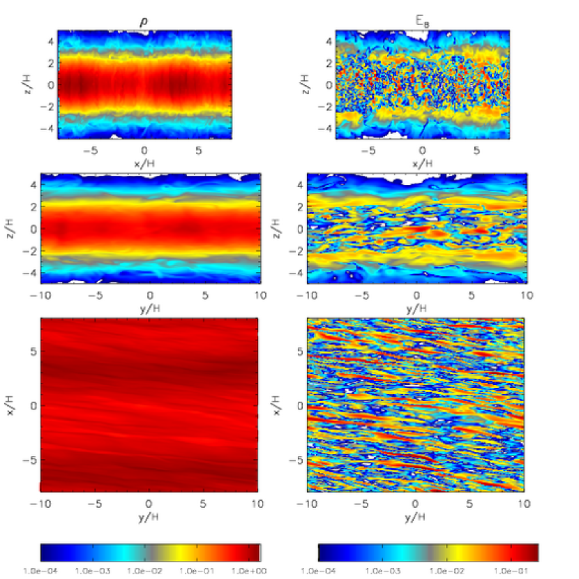
Figure 1: Snapshots of density and magnetic energy density in the fiducial model, taken at $t=100$ orbits. Left: density $\rho$; right: magnetic energy density $E_{B}$; top: image at $y=0$ plane; middle: image at $x=0$ plane; bottom: image at $z=0$ plane.

Our fiducial model has a domain size of $(L_{x},L_{y},L_{z})=(16,20,10)H$ and resolution $384\times 256\times 128$. This corresponds to a physical resolution of $(24,12.8,12.8)$ zones per scale height. Snapshots of $\rho$ and $E_{B}\equiv B^{2}/8\pi$ at slices with constant $x,y$ and $z$ in the saturated state are shown in Figure 1.

Turbulence is confined to the region $|z|\leq 2H$. Within this region magnetic field fluctuations are contained on a scale $l\ll H$, with a structure in the shape of narrow filaments that are extended by the azimuthal shear. This turbulent field structure resembles that observed in unstratified disk simulations (Guan & Gammie, 2009). Density fluctuations on a scale $\sim H$ due to sound waves are also evident in the $x-z$ plane density snapshots. At $|z|>2H$ the MRI is suppressed. $E_{B}$ decreases sharply, but not as rapidly as $\rho$.

The disk vertical structure is shown in Figure 2, which shows $\overline{[\rho]}$, $\overline{[E_{B}]}$, $\overline{[\beta]}$, Maxwell (magnetic) stress $\overline{[M_{xy}]}\equiv\overline{[-B_{x}B_{y}]}/4\pi$ and Reynolds stress $\overline{[R_{xy}]}=\overline{[\rho v_{x}\delta v_{y}]}$. These profiles are obtained from a time average over the last $100\pi/\Omega$. The most striking feature in these profiles is the “turbulent disk surface” at $|z|\sim 2H$ defined by $\overline{[E_{B}]}(z)$ and $\overline{[M_{xy}]}(z)$. Inside this surface both are independent of $z$; outside both exhibit an approximately exponential dependence on $z$. As illustrated in the vertical profile of $\beta$, as $|z|$ increases, magnetic energy density drops slower than density; above $|z|\sim 2.5H$ $\beta$ drops below unity. Therefore the region $|z|>2H$ is magnetically dominated and this leads to the suppression of the MRI. From now on we will simply refer to the magnetically dominated upper region with $\beta<1$ as “corona”, and the turbulent $|z|\leq 2H$ region as ”disk.”

Fits to the disk structure give

$$\overline{[\rho]}(z)\simeq\cases{0.93\rho_{o}\,\exp(-\frac{z^{2}}{2H}),&if $|z|\leq 2.55H$;\cr 0.036\rho_{o}\,\exp{(-\frac{|z|-2.6H}{0.44H})},&otherwise.\cr}$$ (7)

and

$$\overline{[E_{B}]}(z)\simeq\cases{0.012\rho_{0}c_{s}^{2},&if $|z|\leq 2.55H$;\cr 0.012\exp{(-\frac{|z|-2.6H}{0.64H})}\rho_{0}c_{s}^{2},&otherwise.\cr}$$ (8)

In the saturated state, $\overline{[\rho]}(z)$ is different from the initial density profile $\rho_{0}\exp[{-z^{2}/(2H^{2})}]$ due to the magnetic buoyancy effects and mass loss through the $z$ boundaries. Inside the disk, a nearly Gaussian density profile indicates that this region is still mainly supported by gas pressure.

How can we understand the vertical magnetic structure of the disk? A uniformly magnetized atmosphere is subject to interchange and Parker type modes (Newcomb, 1961; Parker, 1966). The more dangerous of these is Parker, whose stability condition is

$$-\frac{d\rho}{dz}>\frac{\rho^{2}g}{\gamma P_{\rm gas}},$$ (9)

where $P_{\rm gas}$ is the gas pressure, $g=\Omega^{2}z$ is the gravitational acceleration, and $\gamma$ is the adiabatic index (here, $\gamma=1$) (Newcomb, 1961). For a disk in hydrostatic equilibrium

$$-\frac{d(P_{\rm gas}+P_{\rm mag})}{dz}=\rho g;$$ (10)

together these conditions imply

$$\frac{dP_{\rm mag}}{dz}=\frac{dE_{B}}{dz}=0.$$ (11)

Marginally stable stratification therefore corresponds to constant $\overline{[E_{B}]}$, as is found at $|z|<2H$. This suggests that (1) magnetic buoyancy is driving the disk toward a marginally stable state; (2) magnetic buoyancy is crucial in controlling the vertical magnetic structure in the bulk of the disk. If this is correct, it follows that $E_{B}(z)$ in the disk could be different in nonisothermal models. In particular, marginal stability requires

$$\frac{1}{8\pi}\frac{d[B^{2}]}{dz}=\gamma P_{gas}\left(\frac{1}{\gamma}\frac{d\ln P_{\rm gas}}{dz}-\frac{d\ln\rho}{dz}\right).$$ (12)

Thus an isentropic disk has $dB^{2}/dz=0$, while a stably stratified, nonradiative disk (in the Schwarzschild sense) can support $dB^{2}/dz<0$. In a radiative disk the instability criterion is modified (disks heated by internal dissipation of turbulence rather than external irradiation tend to have strong radiative diffusion, or Peclet numbers of order $\alpha^{-1}\sim 50$), because radial radiative diffusion tends to wipe out temperature perturbations for the most unstable modes with high radial wavenumbers.

Figure 3 shows the evolution of magnetic energy density in the disk ${\langle}E_{B,{\rm d}}{\rangle}$, magnetic energy density in the corona ${\langle}E_{B,{\rm c}}{\rangle}$ and ${\langle}\alpha{\rangle}$

$${\langle}\alpha{\rangle}\equiv\frac{\int W_{xy}d^{3}x}{\int\rho c_{s}^{2}d^{3}x}$$ (13)

where $W_{xy}\equiv R_{xy}+M_{xy}$ is the total shear stress Averaging the last $50$ orbits, we found that $\overline{{\langle}\alpha{\rangle}}\sim 0.013$, $\overline{{\langle}E_{B,{\rm d}}{\rangle}}/\rho_{0}c_{s}^{2}\sim 0.012$, $\overline{{\langle}E_{B,{\rm c}}{\rangle}}/\rho_{0}c_{s}^{2}\sim 0.0043$.

3.2 Two-point correlation function

One question motivating this study was whether thin disks exhibit mesoscale structure, i.e. structure on scales that are $\gg H$ but $\ll R$. As is evident in Figure 1, the characteristic scale of the magnetic energy density varies with $|z|$. Near $|z|=0$, turbulent structure resembles that observed in unstratified disk models: the field is confined in small structures with scale $l\ll H$. Away from $|z|=0$, $l$ increases, reaching $\sim H$ at $|z|\sim 2.5H$.

The two-point correlation function $\xi$ provides a quantitative measure of disk structure:

$$\xi_{B}(z)\equiv[\delta\mbox{\boldmath$B$}(x,y;z)\cdot\delta\mbox{\boldmath$B$}(x+\Delta x,y+\Delta y;z)].$$ (14)

Here $\delta\mbox{\boldmath$B$}\equiv\mbox{\boldmath$B$}-[\mbox{\boldmath$B$}]$; for a detailed discussion of $\xi$ and the corresponding correlation lengths $\lambda_{i}$ see (Guan et al., 2009). Figure 4 shows $\xi_{B}(z)$ in the $(\Delta x,\Delta y)$ plane at $z=0$, $z=2.5H$ and $z=4.5H$. In these plots we have averaged 8 neighboring vertical zones to increase the signal-to-noise ratio. At the disk midplane, the correlation function has a narrow elliptical core of width $\lambda<$ a few $H$. As $|z|$ increase to $2.5H$ the core becomes larger, especially in the radiation direction, and low amplitude features develop on scales of $\sim 10H$. These low-amplitude, mesoscale features are new and are not seen in unstratified disk models.

3.3 Coronal loop structure

Our disk models contain a “corona”, where $\beta<1$. It is not clear how accurately, or inaccurately, our code models this region because it contains no explicit model for reconnection (nor is any convincing model currently available; see Uzdensky & Goodman (2008) for a discussion of the difficulties of simulating force-free coronae). Still, it is interesting to characterize the field structure in existing simulations before asking how they might be changed by more sophisticated reconnection models.

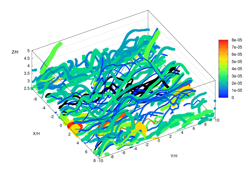
Figure 5: Magnetic field lines originating from the plane $z=2.5H$ in the fiducial model at $t=600\Omega^{-1}$. The lines are evenly sampled spatially from the $x-y$ plane. Both the line width and the color (see the online version for a color version of this plot) denote the flux carried by each line at the footpoint, normalized by the total flux from the $z=2.5H$ plane. Majority of the field lines return to $z=2.5H$, forming closed loops.

How can we understand coronal magnetic field structure? Most of the coronal field is anchored in the disk, so we begin by sampling field lines that rise through the surface $z=2.5H$ at a single instant. Using bilinear interpolation for the field, we trace field lines initiated from every cell on the $z=2.5H$ surface, until they either (a) come back to the $z=2.5H$ surface, or (b) leave the upper $z$ surface, or (c) exceed maxmum integration step $10^{5}$ indicating the formation of a closed loop. A snapshot of these field lines are show in Figure 5. Two features of the coronal field are obvious just from visual inspection: many of the field lines return to the disk after only a short sojourn in the corona, and the loops tend to have greater azimuthal than radial extent.

A more quantitative approach is to calculate a coronal loop distribution function, as in the phenomenological model of Uzdensky & Goodman (2008) (hereafter UG). The field lines should then be sampled according to the flux through each zone surface $d\Phi_{i}=B_{z,i}dxdy$. We also average over the last 50 orbits to improve the loop statistics. We find that $\sim 96\%$ of the field lines passing through the $z=2.5H$ surface return to the same surface, $\sim 4\%$ of field lines are open in the sense that the escape through the upper boundary of the box, and only $\sim 0.1\%$ of the field lines form closed loops inside the corona. We have also found that the small fraction of the open field lines is quite stable during the saturated state, ranging from $\sim 2-5\%$ at instaneous state, therefore it appears that the corona fields structure has reached a statistical steady state.

We then use three variables to describe the geometry of close field lines (field loops) that return to the $z=2.5H$ surface: the loop foot point separation $\Delta\mbox{\boldmath$x$}$ in the $x-y$ plane, the loop maximum height $\Delta z_{\rm max}$, and the loop orientation angle $\theta_{\rm foot}\equiv$ the angle between the foot separation vector and the $y$ axis. We calculate the distributions functions ${d\Phi}/{d\Delta x}$, ${d\Phi}/{d\Delta y}$, ${d\Phi}/{d\Delta z_{\rm max}}$ and ${d\Phi}/{d\theta_{\rm foot}}$ by following the trajectory of every field line that emerges at the center of each zone surface $i$, then weighting the result by the flux $d\Phi_{i}$. The final distribution function is normalized by $|\Phi|$, the total absolute flux through the $z=2.5H$ plane.

Figures 6 and 7 show ${d\Phi}/{d\Delta x}$, ${d\Phi}/{d\Delta y}$, ${d\Phi}/{d\Delta z_{\rm max}}$ and ${d\Phi}/{d\theta_{\rm foot}}$, averaged over the last $50$ orbits. From ${d\Phi}/{d\theta_{\rm foot}}$ (Figure 6) it is evident that most of the field loops are orientated in the azimuthal direction with $\theta\leq$ a few degrees. This suggests that shear plays a significant role in determining the coronal field structures. Most loops also have maximum height $\Delta z_{\rm max}\leq H$ (see ${d\Phi}/{d\theta_{\rm foot}}$ in Figure 7).

If there is no reconnection at all then magnetic energy injection from the underlying turbulent disk might cause the loop to grow in an unlimited way. This is not the case here: although we do not include dissipation explicitly, numerical reconnection due to truncation errors is present in our numerical scheme, as in all finite-difference MHD schemes. It is difficult, however, to quantify the numerical reconnection rate in our model directly. We therefore try to compare our numerical loop distributions to the predictions of the UG model.

We fit a power-law to ${d\Phi}/{d\Delta x}$ and ${d\Phi}/{d\Delta y}$,

$$\frac{d\Phi}{d\Delta x}\simeq C_{0}(\frac{\Delta x}{H})^{k}\,\,,$$ (15)

where $C_{0}$ is a constant. Notice the shape for ${d\Phi}/{d\Delta x}$ and ${d\Phi}/{d\Delta y}$ are very similar. For $\Delta y$ a fit between $3H\leq\Delta y\leq 20H$ gives $k\approx-1.2$. We can also calculate the general loop distribution function for $\Delta L=(\Delta x^{2}+\Delta y^{2})^{1/2}$. It almost overlaps with the ${d\Phi}/{d\Delta y}$ curve because the loops are nearly toroidal, and a fit between $3H\leq\Delta y\leq 20H$ gives $k\approx-1.2$.

In the model of UG, a slope of $k\sim-2$ corresponds to the limit that reconnection is slow compared to the shear (the dimensionless reconnection parameter $\kappa\sim 0.01$ in UG), and a slope of $k>-1.5$ corresponds to the cases when the total magnetic energy of the corona is dominated by the largest loops ($\kappa<0.002$). The shallow $k\sim-1.2$ slope measured here then indicate our numerical models are probably in a slow Sweet-Parker reconnection regime. However, this comparison should not be taken too seriously because our model is ideal MHD, and does not explicitly model reconnection. One serious concern is that the coronal reconnection could fall into a fast, collisionless regime which is poorly understood, and not well modeled by our grid scale dissipation.

Lastly we want to comment on several surface effects in our model. These include the $yz$ component of magnetic stress tensor $M_{yz}\equiv-B_{y}B_{z}/(4\pi)$, the vertical components of kinetic flux and Poynting flux, and the mass loss rate. Notice these quantities do not necessarily average to zero because of the outflow boundary conditions. We have found that ${\langle}M_{yz}{\rangle}$ is nearly zero with temporal fluctuations of amplitude $\leq 10^{-4}\rho_{0}c_{s}^{2}$, much smaller than the dominant $xy$ component ${\langle}M_{xy}{\rangle}$. In the steady state, the vertical energy flux is dominated by the advective part of the Poynting flux, which is on the order of $10^{-4}\rho_{0}c_{s}^{3}$. This vertical energy flux is only $\sim 1\%$ of the turbulent dissipation rate $Q$ in the disk main body ($Q\sim\alpha\rho_{0}c_{s}^{3}\sim 10^{-2}\rho_{0}c_{s}^{3}$), indicating a weak vertical energy flux.

The disk loses mass through the upper and lower boundaries. In the last $50$ orbits, the disk lost $\sim 1.4\%$ of its initial mass. The vertical mass loss rate is not negligible in our $L_{z}=10H$ models because of the outflow boundary conditions. However, we have noted a trend in which the vertical mass loss decreases with increasing $L_{z}$. For example, in our $L_{z}=12H$ model the disk lost $\sim 0.64\%$ of its initial mass during the last $50$ orbits, giving a mass loss rate half that of the $L_{z}=10H$ model. We therefore expect a decreasing mass loss rate as $L_{z}$ increases.

It is also worth noting that in our models the mean vertical magnetic fields maintain ${\langle}B_{z}{\rangle}=0$ because of the shearing box boundary conditions. We also found that the plane-averaged $[B_{z}]\sim 0$ at all $z$ including at the domain boundaries. The vertical field at the surfaces are turbulent with patches of opposite sign field penetrating the boundaries. However the vertical field here are fluctuations with radial correlation length $<$ a few $H$ and amplitude $\sim$ one order of magnitude smaller than that at the disk mid plane. We have not observed a steady magnetic wind and the observed mass loss is probably due to outflow boundaries.

To summarize, in our models we see a weak wind launched from the disk surface. In a steady state both vertical energy and momentum flux are negligible.

3.4 Dependence on Model Parameters

Here we give a brief discussion of the saturation dependence on model parameters, including: (1) resolution; (2) $L_{x}$; (3) $L_{z}$; (4) initial field strength in terms of plasma parameter $\beta_{0}$. When exploring parameter space we vary only one parameter at a time unless stated otherwise. Model parameters can be found in Table 1.

(1) Resolution. In model s16a, we test the convergence properties of our numerical models by doubling the resolution of the fiducial run to $768\times 512\times 256$. We run this model to $t_{f}\sim 75$ orbits. Averaging over the last $\sim 25$ orbits in the satuated state, we found that $\overline{{\langle}\alpha{\rangle}}\sim 0.023$, almost double of that in the fiducial run ($\overline{{\langle}\alpha{\rangle}}\sim 0.013$); at the highest resolution explored in this work, saturation level continues to increase with resolution. The dynamic range in resolution explored in this work is modest (highest resolution in this work is $\sim 20-40$ zones per $H$) due to the computational demands of the large box. We have also monitored “quality factor ” $Q$, where $Q_{i}\equiv\lambda_{\rm MRI,i}/\Delta x_{i}=2\pi v_{\rm a,i}/(\Omega\Delta x_{i})$ (see a discussion of $Q$ in Noble et al. (2010)), the zones per most unstable linear MRI wavelength in our calculations. For the bulk of the disk inside $\pm 2H$ region, our highest resolution run gives a volume and time averaged $Q_{y}=33.7$ and $Q_{z}=6.8$ in the saturated state, and so by this measure the toroidal field MRI is well-resolved while the vertical field MRI is marginally resolved. Of course, the evolution of the disk is not well described by linear theory in the fully turbulent state, so it is not clear whether $Q$ is a good indicator of when MRI-driven turbulence is sufficiently resolved.

It is worth mentioning the convergence properties of shearing box simulations done in smaller boxes: (a) the unstratified box with a net toroidal field, (b) the stratified box with periodic vertical boundary conditions and (c) the stratified box with outflow boundaries. First, using a similar algorithm in unstratified disk simulations with a mean toroidal field, Guan et al. (2009) reported that in the resolution range $32-256/H$ saturation energy increases with resolution ($\propto N_{x}^{1/3}$). They also pointed out that convergence is expected at higher resolution when the energy containing eddies are resolved. For the stratified disks, (Shi, Krolik, & Hirose, 2010) used $L_{x}=2H$ stratified shearing boxes simulations with vertical outflow boundaries and they also found that $\overline{{\langle}\alpha{\rangle}}$ increases with resolution and an $\overline{{\langle}\alpha{\rangle}}\sim 0.035$ in their highest resolution run at $32/H$. Recently, stratified disk simulations done in smaller boxes ($L_{x}\sim H$) and periodic boundary conditions with zero-net flux have demonstrated convergence with $\overline{{\langle}\alpha{\rangle}}\sim 0.01$ with a resolution $\sim 32-128/H$ using ATHENA code and periodic boundary conditions (Davis et al., 2010). The sustained turbulence may be due to the presence of a mean toroidal field in the disk midplane. Notice that $\overline{{\langle}\alpha{\rangle}}$ in their work is normalized with the initial midplane pressure $P_{0}$, which is normally a factor of a few larger than domain-averaged ${\langle}P{\rangle}$ used here. Using the definition in this work, their$\overline{{\langle}\alpha{\rangle}}\sim 0.04$. It is therefore possible that in stratified disk simulations, net-toroidal-field and zero-net-flux models will have similar convergence properties. If this is the case, we then expect a convergence at $64-256/H$ using our ZEUS-type code.

(2) $L_{x}$. For $L_{x}$, we have carried out runs with $L_{x}=H,8H$, and $32H$, denoted by s1, s8, and s32. Time averaging the last $50$ orbits in each run, we found the saturation level in all these runs are close, with $\overline{{\langle}\alpha{\rangle}}\sim 0.0191\pm 0.00453$ when $L_{x}=H$, $\overline{{\langle}\alpha{\rangle}}\sim 0.0124\pm 0.00116$ when $L_{x}=8H$, $\overline{{\langle}\alpha{\rangle}}\sim 0.0125\pm 0.000965$ when $L_{x}=16H$, and $\overline{{\langle}\alpha{\rangle}}\sim 0.0269\pm 0.00211$ when $L_{x}=32H$, where the numbers after $\pm$ denotes standard deviation $\sigma$. The dependence of $\overline{{\langle}\alpha{\rangle}}$ on the box size is not clear, however, it is difficult to measure $\overline{{\langle}\alpha{\rangle}}$ in the $L_{x}=H$ box because of the large fluctuations. In runs with $L_{x}\geq 8H$, the $\sigma$-to-mean ratio is aroud $0.07-0.09$, while $L_{x}=H$ gives a $\sigma$-to-mean ratio $\sim 0.25$.

Past stratified disk studies ((Davis et al., 2010; Shi, Krolik, & Hirose, 2010)) have shown that there exist significant (order of unity) long term fluctuations in $L_{x}\sim H$ box. The evolution of magnetic energy density in the disk ${\langle}E_{B,d}{\rangle}$ for $L_{x}=H$ and $L_{x}=16H$ runs are shown in Figure 8. The smaller fluctuation in large $L_{x}$ models suggest that: (a) parts of the disk with horizontal separation $>H$ are uncorrelated, and (b) the volume integration over large-enough domain will smooth out these local fluctuations.

What have we learned in these large domain size models with $L_{x}\geq 10H$? Our $L_{x}=H$ run is similar to the toroidal model of Miller & Stone (2000). First, in large box runs, the plane-averaged vertical disk structures are similar to those in smaller box runs: we have observed a gas-pressure supported disk with a Gaussian density profile inside $\sim 2H$ and an extended magnetic dominated corona outside $\sim 2H$. Second, the long-term average of disk turbulence saturation level is also very similar to the $\sim H$ runs, albeit with much smaller temporal fluctuations. Statistically, for saturation measurement purposes, a large domain run can be regarded as a sum of smaller $H$ run, where the temporal and spatial fluctuations are smoothed out by integrating over decorrelated disk regions.

Our models also suggest that a magnetically dominated corona cannot be studied in an $L_{x}\sim H$ box (if it can be studied in a numerical MHD model at all). In large domain size runs with $L_{x}\geq 10H$ at $|z|>2H$ we find features in the magnetic field correlation function on scales of $\sim 10H$, indicating the existence of meso-scale structure. Although the magnitude of the mass, angular momentum and energy transport in the corona is small compared to that in the central disk, the corona and the central disk are dynamically connected and large scale structure in magnetically dominated upper layers may still influence the spatial correlations/structures of the disk below (we will explore this issue in a forthcoming paper). Therefore, in accretion disk models where the spatial structure of the corona is important, such as phenomenological models for accretion disk coronae (e.g., the statistical model of Uzdensky & Goodman 2008) and disk spectra calculations, the radial extent of the corresponding numerical simulation may require a $L_{x}\geq 10H$.

(3) $L_{z}$. We have investigated the effect of vertical boundaries by running a model (s16c) with $L_{z}=12H$. We find no qualitative difference between the $L_{z}=12H$ and $L_{z}=10H$ models: the saturation $\overline{{\langle}\alpha{\rangle}}\sim 0.0141$, $\overline{{\langle}E_{B,{\rm d}}{\rangle}}/\rho_{0}c_{s}^{2}\sim 0.0125$, and $\overline{{\langle}E_{B,{\rm c}}{\rangle}}/\rho_{0}c_{s}^{2}\sim 0.00497$, all within $\sim 10\%$ of the fiducial model. We also obtain a similar vertical disk structure when $L_{z}$ increases: inside $2.5H$ the disk has a well-fitted Gaussian $\overline{[\rho]}(z)$ and a flat $\overline{[E_{B}]}(z)$; outside $2.5H$ the corona extends to $|a|=\pm 6H$ in model s16c. Both $\overline{[\rho]}(z)$ and $\overline{[E_{B}]}(z)$ also have an exponential profile, but the fitted coronal exponential scale height increases $\sim 20\%$ compared to the fiducial model. The coronal loop distribution functions are almost identical to those of the fiducial model, which is not suprising considering the steep decline of ${d\Phi}/{d\Delta z_{\rm max}}$ as $\Delta z_{\rm max}$ exceeds $\sim H$. As discussed before, some caution is needed in interpreting this vertical extension of corona structure with increasing domain size: our calculation is essentially a MHD calculation, whereas real disk coronae are probably force-free and also influenced by non-ideal plasma effects (e.g., reconnection) that are ill-modeled in our numerical scheme.

(4) $\beta_{0}$. We have tested the effect of initial field strength on the saturation level. In most of our runs we start from a uniform toroidal field inside the disk with $\beta_{0}=25$. We then carry out a comparison run s16b with the same field geometry but weaker strength $\beta_{0}=100$. We find that turbulence saturates at the similar level using weaker initial field strength, with $\overline{{\langle}\alpha{\rangle}}\sim 0.0157$, $\overline{{\langle}E_{B,{\rm d}}{\rangle}}/\rho_{0}c_{s}^{2}\sim 0.0152$, and $\overline{{\langle}E_{B,{\rm c}}{\rangle}}/\rho_{0}c_{s}^{2}\sim 0.00647$, therefore in stratified disks the saturation does not depend on the initial field strength.

In comparison, in unstratified disk models ${\langle}E_{B}{\rangle}$ is found to scale with the initial mean field strength ${\langle}B_{y}{\rangle}$ (see a detail discussion in Guan et al. 2009). The important difference here lies in the stratification and the accompanying outflow boundary conditions, which allow changes in mean toroidal field strength in the turbulent disk. The stratified disk model then allows the disk to adjust its net flux and field strength in a self-consistent way. It is worth pointing out that the saturation level is a volume average over large scales where different parts of the disk decorrelate; on the scale where the turbulence is localized ($\leq H$), it is still possible that the local saturation ${\langle}E_{B,{\rm d}}{\rangle}_{\rm local}\propto{\langle}B_{y,{\rm d}}{\rangle}_{\rm local}$.

Does the saturation level depend on the instantaneous mean field strength in the stratified disk? The evolution of the mean azimuthal field ${\langle}B_{y,{\rm d}}{\rangle}$ in the region $|z|\leq 2H$ in model s32 is plotted in Figure 9. The mean field does not have a fixed value and changes signs over a time scale of $\sim 10$ orbits. Averaging the last $100$ orbits, the mean magnitude of toroidal field strength in the turbulent disk region is $\overline{|{\langle}B_{y}{\rangle}|}\sim 0.012\sqrt{4\pi}\rho_{0}^{1/2}c_{s}$, therefore there is weak net toroidal field in the turbulent disk region to drive MRI. The figure also shows the evolution of the mean magnetic energy density ${\langle}E_{B,{\rm d}}{\rangle}$ and mean $xy$ stress ${\langle}W_{xy,{\rm d}}{\rangle}$ in the same run. Both ${\langle}E_{B,{\rm d}}{\rangle}$ and ${\langle}W_{xy,{\rm d}}{\rangle}$ have a fixed overall saturation level with a superimposed small oscillation with a period half of that of ${\langle}B_{y}{\rangle}$. Again, this is dramatically different from the unstratified disk, where the saturation level is proportional to the mean field strength. The overall saturation level in a stratified disk is ${\it not}$ determined by the instantaneous mean field strength, nor by the initial field strength.

On the other hand, as shown in Figure 9, the oscillations of ${\langle}B_{y}{\rangle}$ and ${\langle}E_{B,{\rm d}}{\rangle}$ are closely correlated and oscillation period for ${\langle}B_{y}{\rangle}$ is twice that of ${\langle}E_{B,{\rm d}}{\rangle}$. This suggests that ${\langle}B^{2}{\rangle}$ is correlated with ${\langle}B_{y}{\rangle}$, even though ${\langle}B_{y}{\rangle}\ll{\langle}B^{2}{\rangle}^{1/2}$. Therefore, the saturation level may be determined both by the MRI induced by the mean toroidal field in the turbulent disk region and magnetic buoyancy effects (e.g., Vishniac (2009)).

4 Butterfly Diagram: A Mean Dynamo In the Disk?

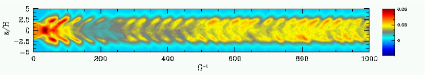
Figure 10: Butterfly diagram for $[E_{B}]$ in the model s32.

One interesting feature appearing in all our models is an oscillation of the mean magnetic energy on a timescale of a few orbits. As an example, we plot the “butterfly” diagram for model s32 in Figure 10, which illustrates the evolution of $[E_{B}](z)$. This bears a superficial resemblance to the famous butterfly diagram observed in solar activity cycles.

We use Fourier analysis to determine the period of butterfly diagram. Using data $\int dyE_{B}(|z|=2.5H;x,t)$, taken from two layers with $|z|\sim 2.5H$ and have been averaged in $y$ direction to improve statistics, we perform a two dimensional FFT (in $x$ and $t$) on the data set. The normalized temporal power spectral density (PSD) for $[E_{B,|z|=2.5H}]$ in model s32 are shown in Figure 11. Here we have plotted a cut through $k_{x}=0$ plane in the 2D $k_{x}-f$ PSD map. We have also checked that the different sides of the disk have very similar PSD and we have plotted the sum of contribution from both layers. The arrow in the figure marks the peak frequency in the PSD. This frequency, $f\sim 0.03\Omega$ corresponds to the period of the butterfly diagram for $[E_{B}]$.

The PSD has $P\sim f^{k}$, with $k\sim-2.3$. Interestingly, results from recent global GRMHD simulations (Noble & Krolik, 2009) suggest that the slope for the coronal luminosity temporal power spectrum is $k\sim-2$, almost independent of model parameters and very close to what has been observed at high frequency in black hole accretion disk systems. The power-law index for the temporal power spectrum from local and global simulations are therefore remarkably close, considering we are only calculating the temporal spectrum for coronal magnetic energy density.

The period for $[E_{B}]$ is $P_{[E_{B}]}\sim 5$ orbits. Besides $[E_{B}]$, one could also plot butterfly diagrams for $[W_{xy}]$ and $[B_{y}]$. The period for $[W_{xy}]$ is the same as that of $[E_{B}]$, $\sim 5$ orbits, while the period for $[B_{y}]$ is twice that of $[E_{B}]$, $P_{[B_{y}]}\sim 10$ orbits, because of the reversal of mean fields (see Figure 9).

For $[E_{B}]$, we find $P_{{\langle}E_{B}{\rangle}}\sim 5$ orbits in all our models. This quasi periodicity has appeared in all the stratified shearing box simulations that we are aware of, even in those with periodic vertical boundary conditions (Stone et al., 2009). Interestingly, Reynolds & Fabian (2008) has also obtained similar butterfly diagrams at certain radii (e.g., $r=8r_{g}$ and $r=10r_{g}$, where $r_{g}\equiv GM/c^{2}$ is the gravitational radii) in their global pseudo-Newtonian thin disk simulations. It would be of interest in the future to test (a) whether the butterfly diagram is simply a local feature at a certain location on the disk (as in shearing box simulations) or this quasi-periodicity can be coherent and sustained over a large radial range, and (b) what model parameter(s) the period depends on.

The butterfly diagram together with the reversal of the mean fields (for both the dominant toroidal field and a weak radial field) in the disk may be modeled by a mean field dynamo of $\tilde{\alpha}$ type (e.g., Moffatt (1978)). In the rest of this section, we will present a toy model to give a qualitative description of these oscillations.

Let us first consider two important dynamical processes in a stratified disk: (1) the MRI-driven turbulence, which draws free energy of rotation and operates on the orbital timescale $\sim\Omega^{-1}$; (2) magnetic buoyancy, which operates on the local Alfvén timescale $\tau_{\rm A}\sim H/[\delta v_{A}^{2}]^{1/2}$. In our simulations we found in the disk region $|z|\leq 2H$ the magnetic energy density is almost a constant with height, with $[E_{B}]\geq 10^{-2}\rho_{0}c_{s}^{2}$, which gives an average magnetic buoyancy timescale $\tau_{\rm A}\leq$ a few $\Omega^{-1}$ inside the disk. The period of the butterfly diagram is much longer than these two timescales. Therefore these two processes alone can not describe the dynamics represented in butterfly diagrams.

The $\tilde{\alpha}$ type mean dynamo equations for the disk mean fields ${\langle}B_{x}{\rangle}$ and ${\langle}B_{y}{\rangle}$ can be derived from averaging the induction equation, $\partial_{t}{{\langle}\mbox{\boldmath$B$}{\rangle}}={\langle}\nabla\times({\mbox{\boldmath$v$}}\times{\mbox{\boldmath$B$}}){\rangle}$, here ${\langle}\,\,{\rangle}$ denotes ensemble averages. Assuming the turbulent EMF $\varepsilon$ is related to the mean field with a dynamo parameter $\tilde{\alpha}_{i}$, ${\langle}{\mbox{\boldmath$\varepsilon$}}{\rangle}\equiv{\langle}{\delta\mbox{\boldmath$v$}}\times{\delta\mbox{\boldmath$B$}}{\rangle}=\tilde{\alpha}_{i}{\langle}{\mbox{\boldmath$B$}}_{i}{\rangle}$, one simple form of dynamo equations in a stratified thin Keplerian disk is (cf., Eqn (5-6) in Vishniac& Brandenburg (1997)),

$$\partial_{t}{\langle}B_{y}{\rangle}=-\frac{3}{2}\Omega{\langle}B_{x}{\rangle}-\partial_{z}({\langle}v_{\rm b}{\rangle}{\langle}B_{y}{\rangle})+\partial_{z}(\tilde{\alpha}_{1}{\langle}B_{x}{\rangle})\,\,,$$ (17)

and

$$\partial_{t}{B_{x}}=-\partial_{z}({\langle}v_{\rm b}{\rangle}{\langle}B_{x}{\rangle})-\partial_{z}(\tilde{\alpha}_{2}{\langle}B_{y}{\rangle})\,\,,$$ (18)

where $v_{\rm b}$ is a characteristic vertical velocity induced by magnetic buoyancy. In Eqn (17) the first term is the shear term, second term denotes buoyancy due to the mean field, and the last term is the mean field dynamo term. Only $\partial_{z}$ terms are retained because the disk is thin. For simplicity we have also dropped the diffusion terms. We then take $\partial_{z}\sim 1/(2H)$ and $v_{\rm b}\approx|v_{A}|\equiv|B|/\sqrt{4\pi\rho_{0}}\sim|B_{y}|/\sqrt{4\pi\rho_{0}}$, where $|v_{A}|$ is the mean Alfvén speed. Eqn(17) and Eqn(18) then become

$$\frac{dB_{y}}{dt}=-\frac{3}{2}\Omega B_{x}-\frac{|v_{A}|}{2H}B_{y}+\frac{\tilde{\alpha}_{1}}{2H}B_{x}\,\,,$$ (19)

and

$$\frac{dB_{x}}{dt}=-\frac{|v_{A}|}{2H}B_{x}-\frac{\tilde{\alpha}_{2}}{2H}B_{y}\,\,.$$ (20)

For clarity we have dropped ${\langle}\,\,{\rangle}$ in the above equations. Notice that Eqn (19) and Eqn (20) have no spatial dependence. Taken together, they are coupled ODEs and can be solved numerically given initial conditions for $B_{y}$ and $B_{x}$.

In Figure 12 we plot one solution for this toy model. This solution is obtained by integrating the above equations from an initially pure toroidal field with $\beta_{0}\sim 22$ and by choosing $\tilde{\alpha}_{1}=\tilde{\alpha}_{2}=-0.01$. The period for $B_{y}$ in this particular toy model is $\sim 10$ orbits. The magnitude of $\tilde{\alpha}$ controls the oscillation frequency: in general, larger $|\tilde{\alpha}|$ leads to smaller period, although the scaling is not linear. Initial conditions have little effect on the evolution in our toy model. In conclusion, the butterfly diagram and the mean field reversal observed in these simulations may imply a mean field dynamo at work in stratified disks.

Does it make sense to identify these oscillations with observed QPOs? In a Keplerian disk the orbital frequency at $r$ is $f_{\rm orb}=1/(2\pi)(GM)^{1/2}r^{-3/2}$. The QPO frequency is $f_{\rm QPO}=1/5f_{\rm orb}\approx 20\times(r/10M)^{-3/2}(M/10{\rm\,M_{\odot}})^{-1}{\rm Hz}$. Our disk model represents a geometrically thin, optically thick disk. This is most easily understood as corresponding to the high soft state in black hole X-ray binaries, which is dominated by a thermal component. For a $10{\rm\,M_{\odot}}$ black hole a $5{\rm Hz}$ QPO (e.g., XTEJ1550-564) corresponds to $r_{\rm in}\sim 25M$, which is far from innermost region of a thin disk where most of the thermal X-ray emissions presumably originates. This oscillation frequency may be sensitive to the disk vertical structure (e.g. if the disk is not isothermal), and therefore may exhibit a much more complex behavior in real disks, in which the vertical structure is closely coupled to vertical energy transport. On the other hand, observations indicates that QPOs are absent or very weak in the thermal state, but may appear in the very high state when a sizable thermal disk component is present, although the QPOs are more associated with Comptonizing electrons ((Remillard & McClintock, 2006)); it is difficult to associate the butterfly oscillations with observed QPO phenomena.

5 Summary and Discussion

We have carried out stratified shearing box simulations with domain size $L_{x}=H$ to $L_{x}=32H$ to study properties of isothermal accretion disks on a scale larger than the disk scale height $H$. Our numerical models have vertical extent $\geq 5H$ above and below the disk midplane with outflow boundary conditions. All models start from a net mean toroidal field in the central disk region and the mean fields are allowed to change in the evolution.

We find the disk has an oscillating mean toroidal field and $\overline{{\langle}\alpha{\rangle}}\sim 0.012-0.025$ in the parameter range we explored. We have not found a clear dependence of $\overline{{\langle}\alpha{\rangle}}$ on $L_{x}$ in our models, although the temporal variances in volume averaged quantities decreases with $L_{x}$. The highest resolution used here is modest ($20-40$ zones per $H$), and we have observed $\overline{{\langle}\alpha{\rangle}}$ increases with resolution. Recently, Stone el al. report a converged $\overline{{\langle}\alpha{\rangle}}\sim 0.04$ in $L_{x}\sim H$ high resolution stratified disk simulations with zero-net-flux and periodic vertical boundary conditions (so that the volume-averaged field cannot change during the evolution). The sustained turbulence may be due to the presence of a mean toroidal field in the region close to the disk midplane, lending plausibility to the idea that the saturation mechanism of MRI in stratified disks near the midplane is similar to that in unstratified disks with a net toroidal field.

In the saturated state the disk vertical structure consists of (a) a turbulent disk at $|z|\leq 2H$ and (b) a magnetically dominated upper region at $|z|>2H$, confirming earlier small ($L_{x}\sim H$) box results.

At $|z|\leq 2H$, the disk is mainly supported by gas pressure, and a Gaussian density profile is observed. The plane averaged magnetic energy density $[E_{B}](z)$ and Maxwell stress $[M_{xy}](z)$ are nearly uniform with vertical height $z$ in this region, where the disk is marginally stable to the Parker instability. At $|z|>2H$, exponential dependences on $z$ are observed for both $[\rho]$ and $[E_{B}]$. Fitting formulae for $[\rho](z)$ and $[E_{B}](z)$ are given in Eqn (7) and Eqn (8) respectively.

Using a two-point correlation function analysis, we found that close to the midplane, the disk is dominated by small scale ($\leq H$) turbulence, very similar to what we have observed in unstratified disk models. In the corona, magnetic fields are correlated on scales of $\sim 10H$, implying the existence of meso-scale structures. Recently Johansen et al. (2009) have also observed large scale pressure and zonal flow structures in their large shearing box simulations. We will give a detailed report of meso-scale structure in isothermal disks in a forthcoming paper.

We have adopted a statistical approach to study the geometry of coronal magnetic fields. Only $\approx 4\%$ of coronal field lines are open. For closed field lines, we calculated the magnetic loop distribution function for the loop foot separation $\Delta\mbox{\boldmath$x$}$ in the $x-y$ plane, loop maximum height $\Delta z_{\rm max}$, and loop orientation angle $\theta_{\rm foot}$. The loops are dominantly toroidal due to the differential shear. The loop foot distribution between $H-20H$ is a power law with an index $k\sim-1.25$. In the phenomenological model of UG, this corresponds to the limit where reconnection is slow compared to the shear. These comparisons are limited because our models are working in an ideal MHD regime and reconnection is purely numerical.

In our models both vertical energy and momentum flux are negligible in the steady state. The mass loss rate from the disk surface is small and decreases with increasing $L_{z}$. The surface effects are therefore minimal and indicate a lack of disk winds in our stratified disk models. The weak winds are consistent with the constraint that we have a zero-net vertical magnetic flux in these models. A Blandford-Payne type wind requires the existence of a vertical net field (e.g., see Suzuki & Inutsuka (2009)), although we note that in their models the most unstable wavelength for the extremely weak field are probably not resolved.) Initial investigations show that even a weak ($\beta_{0}\sim 1600$) net z field will induce very violent accretion in stratified shearing box models: at certain region of the disk accretion will run away, eventually causing the disk break into rings. Similar phenomena were reported in net vertical field models of Miller & Stone (2000).

We have confirmed the “butterfly” diagram seen in earlier stratified disk models of size $L_{x}\sim H$. The butterfly diagrams persist even in our largest runs with $L_{x}=32H$. We also report the reversal of the mean fields (for both the dominant toroidal field and a weak radial field) in the disk on a timescale twice that of $[E_{B}]$. The periods for the butterfly diagram are close in all our models, $P\sim 5$ orbits for $[E_{B}]$ and $P\sim 10$ orbits for $[B_{y}]$. The mean field reversal and butterfly diagram may indicate the existence of a mean field dynamo in stratified disks, perhaps controlled by the MRI and magnetic buoyancy. We have presented a toy model for an $\tilde{\alpha}$ type mean field dynamo in stratified disks and found an $\tilde{\alpha}_{\rm imp}\sim 0.01$ will produce the reported period. Further exploration of parameter dependences would be useful for analytical modeling. In the future it would also be interesting to test whether the butterfly oscillations persist when averaging over a large range of radii in global disk simulations. The butterfly diagram may be associated with low frequency QPOs and therefore a good observational diagnostic for accretion flows. On the other hand, we also report a power-law index $k\sim-2.3$ in the temporal power spectrum for coronal magnetic energy fluctuations, consistent with results from recent GRMHD black hole accretion disk simulations.

Our stratified disk models are primarily limited by the assumption that the disk is isothermal. Effects of thermodynamics and radiation therefore are neglected in this work. Our models are also limited by finite resolution, box size, evolution time, and the absense of explicit dissipation. Additional insights may also provided by the future explorations on magnetic field strength and geometry in disks.

Table 1: Model Parameters

Model	Size	Resolution	$\beta_{0}$	$\overline{{\langle}\alpha{\rangle}}$	$\overline{{\langle}E_{B,|z|\leq 2H}{\rangle}}/\rho_{0}c_{s}^{2}$	$\overline{{\langle}E_{B,|z|>2H}{\rangle}}/\rho_{0}c_{s}^{2}$
std16	$(16,20,10)H$	$384\times 256\times 128$	25	0.0125	0.0121	0.00427
s16b	$(16,20,10)H$	$384\times 256\times 128$	100	0.0157	0.0152	0.00647
s16c	$(16,20,12)H$	$384\times 256\times 160$	25	0.0141	0.0125	0.00497
s1	$(1,20,10)H$	$48\times 256\times 128$	25	0.0191	0.0171	0.00933
s8	$(8,20,10)H$	$192\times 256\times 128$	25	0.0124	0.0115	0.00665
s32	$(32,20,10)H$	$768\times 256\times 128$	25	0.0269	0.0270	0.0106
s16a	$(16,20,10)H$	$768\times 512\times 256$	25	0.0230	0.0181	0.0101

Figure 2: Vertical profiles of several $x-y$ plane averaged quantities in the fiducial model. Upper left: density; Upper right: magnetic energy density; Lower left: plasma $\beta$; Lower right: $xy$ component of Maxwell stress $M_{xy}=-B_{x}B_{y}/4\pi$ (solid lines) and Reynolds stress $R_{xy}=\rho v_{x}\delta v_{y}$ (dotted lines). All quantities in solid and dotted lines are averaged from the last $50$ orbits. To illustrate the time average effect, we also plot $[E_{B}](z)$ at $t=900\Omega^{-1}$ (dashed lines) in the upper right panel. The slight asymmetry of $\overline{[E_{B}]}(z)$ and $\overline{[M_{xy}]}(z)$ in the $|z|\leq 2H$ region is probably due to our choice of orbits interval for time average.

Figure 3: Evolution of ${\langle}\alpha{\rangle}$ (solid lines), ${\langle}E_{B,d}{\rangle}/\rho_{0}c_{s}^{2}$ at $|z|\leq 2H$ (dotted lines), and ${\langle}E_{B,c}{\rangle}/\rho_{0}c_{s}^{2}$ at $|z|>2H$ (dashed lines) in the fiducial model. Saturation $\overline{{\langle}\alpha{\rangle}}\sim 0.013$ when averaged over the last $50$ orbits.

Figure 4: Contour plots of 2D two-point correlation function $\xi_{B}(z)$ for $\delta\mbox{\boldmath$B$}$. Plotted are $\xi_{B}(z)/(4\pi\rho_{0}c_{s}^{2})$ in the $(\Delta x,\Delta y)$ plane at three different vertical heights in the fiducial model. Left: mid plane; Middle: $z=2.5H$; Right: $z=4.5H$. The contours run linearly from $-0.058$ to $0.229$ for $20$ levels; solid lines: $\xi_{B}\geq 0$; dash lines: $\xi_{B}<0$; the heavy line is the $0$ contour.

Figure 6: Loop angle distribution functions in the fiducial model: $\theta$ denotes the angle between the foot separation vector and the $y$ axis. Loops are stretched in the azimuthal direction due to the shear.

Figure 7: Loop-distribution functions in the fiducial model. Left panel: foot point separation distribution. Left curve is for $\Delta x$ and Right curve is for $\Delta y$. The distribution for $\Delta L=(\Delta x^{2}+\Delta y^{2})^{1/2}$ almost overlaps with the $\Delta y$ curve. The heavy line indicates a $k=-5/4$ slope. Right panel: loop height distribution.

Figure 8: Evolution of the disk magnetic energy density ${\langle}E_{B,d}{\rangle}$ in the model std16 (solid lines) and s1 (dotted lines). Plotted are the mean magnetic energy density in the region $|z|\leq 2H$.

Figure 9: Evolution of ${\langle}B_{y}{\rangle}$ (solid lines), ${\langle}E_{B}{\rangle}$ (dotted lines) and ${\langle}W_{xy}{\rangle}$ (dashed lines) at $|z|\leq 2H$ in model s32. The oscillation period for ${\langle}B_{y}{\rangle}$ is twice that of ${\langle}E_{B}{\rangle}$ and ${\langle}W_{xy}{\rangle}$. These temporal oscillations may be caused by a mean field dynamo.

Figure 11: Normalized temporal power spectral density for $[E_{B}]$ in the model s32. The data are taken from the layers with $|z|\sim 2.5H$. We also draw the best-fit $k=-2.3$ slope for the temporal PSD. The arrow marks the peak frequency in the power spectrum. This frequency, $f\sim 0.03\Omega$, corresponds to the period of the butterfly diagram for $[E_{B}]$.

.

Figure 12: Evolution of $B_{y}$ (solid lines) and $B_{x}$ (dotted lines) in our mean field dynamo toy model. $\alpha_{1}=\alpha_{2}=-0.01$ in the plotted model.

.

References

- Balbus & Hawley (1991) Balbus, S. A., & Hawley, J. F. 1991, ApJ, 376, 214
- Blandford & Payne (1982) Blandford, R. D. & Payne, D. G. 1982 MNRAS, 199, 883
- Blaes et al. (2006) Blaes, O. M., Davis, S. W., Hirose, S., Krolik, J. H., & Stone, J. M. 2006 ApJ, 645, 1402
- Blaes et al. (2007) Blaes, O., Hirose, S. & Krolik, J. H. 2007 ApJ, 664, 1057
- Brandenburg et al. (1995) Brandenburg, A., Nordlund, Å., Stein, R. F., & Torkelsson, U. 1995 ApJ, 446, 741
- Davis et al. (2005) Davis, S. W., Blaes, O. M., Hubeny, I., & Turner, N. J. 2005, ApJ, 621, 372
- Davis et al. (2010) Davis, S. W., Stone, J. M., & Pessah, M. E. 2010, ApJ, 713, 1
- Fromang & Papaloizou (2007) Fromang, S., & Papaloizou, J. 2007 A&A, 476, 1113
- Fromang & Stone (2009) Fromang, S., & Stone, J. M. 2009, A&A, 507, 19
- Guan & Gammie (2009) Guan, X., & Gammie, C. F. 2009, ApJ, 697, 1901
- Guan et al. (2009) Guan, X., Gammie, C. F., Simon, J. B., & Johnson, B. M. 2009 ApJ, 694, 1010
- Gammie (2001) Gammie, C. F. 2001, ApJ, 553, 174
- Hawley et al. (1995) Hawley, J. F., Gammie, C. F., & Balbus, S. A. 1995, ApJ, 440, 742
- Hirose et al. (2006) Hirose, S. ; Krolik, J. H., & Stone, J. M. 2006, ApJ, 640, 901
- Hirose et al. (2009) Hirose, S. ; Krolik, J. H., & Blaes, O. 2009, ApJ, 691, 16
- Johansen et al. (2009) Johansen, A., Klahr, H., & Youdin, A. 2009, ApJ, 697, 1269
- Johnson & Gammie (2005) Johnson, B. M., & Gammie, C. F. 2005, ApJ, 635, 149
- Johnson et al. (2008) Johnson, B. M., Xiaoyue Guan, & Gammie, C. F. 2008, ApJS, 177, 373
- Krolik et al. (2007) Krolik, J. H.; Hirose, S.; Blaes, O. 2007, ApJ, 664, 1045
- Lesur & Longaretti (2007) Lesur, G. & Longareti, P. Y. 2007, A&A, 378, 1471
- Lightman & Eardley (1974) Lightman, A. P. & Eardley, D. M. 1974, ApJ, 187, 1
- Lynden-Bell & Pringle (1974) Lynden-Bell, D., & Pringle, J. E. 1974, MNRAS, 235, 269
- Masset (2000) Masset, F. 2000, A&AS, 141, 165
- Miller & Stone (2000) Miller, K. A. & Stone, J. M. 2000, ApJ534, 398 (MS00)
- Moffatt (1978) Moffatt, H. K. 1978, Chapter 9, Magnetic Field Generation In Electrically Conducting Fluids. Cambridge University Press, Cambridge
- Newcomb (1961) Newcomb, W. A. 1961, Phys. Fluids, 4, 391
- Noble & Krolik (2009) Noble, S. C. & Krolik, J. H. 2009, ApJ, 703, 964
- Noble et al. (2009) Noble, S. C.; Krolik, J. H., & Hawley, J. F. 2009, ApJ, 692, 411
- Noble et al. (2010) Noble, S. C.; Krolik, J. H., & Hawley, J. F. 2010, ApJ, 711, 959
- Novikove & Thorne (1973) Novikov, I. D., & Thorne, K. S. 1973 , Black Holes, Eds. C De Witt, B S De Witt, Gordon and Breach, London
- Parker (1966) Parker, E. N. 1966, ApJ, 145, 811
- Pessah & Goodman (2009) Pessah, M. E., & Goodman, J. 2009, ApJ, 698, 72
- Piran (1978) Piran, T. 1978, ApJ, 221, 652
- Remillard & McClintock (2006) Remillard, R. A., & McClintock, J. E. 2006, ARA&A, 44, 49
- Reynolds & Fabian (2008) Reynolds, C. S., & Fabian, A. C. 2008, ApJ, 675, 1048
- Shafee et al. (2008) Shafee, R., McKinney, J. C., Narayan, R., Tchekhovskoy, A., Gammie, C. F., & McClintock, J. E. 2008, ApJ, 687, 25
- Shakura & Sunyaev (1973) Shakura, N. I., & Sunyaev, R. A. 1973, A&A, 24, 337
- Shi, Krolik, & Hirose (2010) Shi, J., Krolik, J. H., & Hirose, S. 2010, ApJ, 708, 1716
- Simon & Hawley (2009) Simon, J. B., & Hawley, J. F. 2009, ApJ, 707, 833
- Stone et al. (1996) Stone, J. M., Hawley, J. F., Gammie, C. F., & Balbus, S. A. 1996, ApJ, 463, 656 (SHGB96)
- Stone & Norman (1992) Stone, J. M. & Norman, M. L. 1992, ApJS, 80, 753
- Spruit & Uzdensky (2005) Spruit, H. C., & Uzdensky, D. A. 2005, ApJ, 629, 960
- Suzuki & Inutsuka (2009) Suzuki, T. K., & Inutsuka, S. 2009, ApJ, 691, 49
- Tout & Pringle (1996) Tout, C. A., & Pringle, J. E. 1996, MNRAS, 281, 219
- Turner et al. (2003) Turner, N. J., Stone, J. M., Krolik, J. H., & Sano, T. 2003, ApJ, 593, 992
- Turner (2004) Turner, N. J. 2004, ApJ, 605, 45
- Uzdensky & Goodman (2008) Uzdensky, D. A., & Goodman, J. 2008, ApJ, 682, 608 (UG)
- Vishniac (2009) Vishniac, E. T. 2009, ApJ, 696, 1021
- Vishniac& Brandenburg (1997) Vishniac, E. T. & Brandenburg, A., 1997, 475, 263