Analysis of the 3d massive renormalization group perturbative expansions: a delicate case

Abstract

The effectiveness of the perturbative renormalization group approach at fixed space dimension $d$ in the theory of critical phenomena is analyzed. Three models are considered: the $O(N)$ model, the cubic model and the antiferromagnetic model defined on the stacked triangular lattice. We consider all models at fixed $d=3$ and analyze the resummation procedures currently used to compute the critical exponents. We first show that, for the $O(N)$ model, the resummation does not eliminate all non-physical (spurious) fixed points (FPs). Then the dependence of spurious as well as of the Wilson-Fisher FPs on the resummation parameters is carefully studied. The critical exponents at the Wilson-Fisher FP show a weak dependence on the resummation parameters. On the contrary, the exponents at the spurious FP as well as its very existence are strongly dependent on these parameters. For the cubic model, a new stable FP is found and its properties depend also strongly on the resummation parameters. It appears to be spurious, as expected. As for the frustrated models, there are two cases depending on the value of the number of spin components. When $N$ is greater than a critical value $N_{\mathrm{c}}$, the stable FP shows common characteristic with the Wilson-Fisher FP. On the contrary, for $N<N_{\mathrm{c}}$, the results obtained at the stable FP are similar to those obtained at the spurious FPs of the $O(N)$ and cubic models. We conclude from this analysis that the stable FP found for $N<N_{\mathrm{c}}$ in frustrated models is spurious. Since $N_{\mathrm{c}}>3$, we conclude that the transitions for XY and Heisenberg frustrated magnets are of first order. field theory, renormalization group, critical phenomena, perturbation theory, resummation 75.10.Hk, 11.10.Hi, 12.38.Cy

Abstract

Аналiзується ефективнiсть пертурбативного пiдходу у методi ренормалiзацiйної групи при фiксованiй вимiрностi простору $d$ в теорiї критичних явищ. Розглядається три моделi: $O(N)$, кубiчна i антиферомагнiтна модель означена на трикутнiй ґратцi. Ми розглядаємо усi моделi при фiксованому $d=3$ i аналiзуємо процедуру пересумовування, яка використовується для обчислення критичних показникiв. Ми спочатку показуємо, що для $O(N)$ моделi пересумовування не виключає усi нефiзичнi (фiктивнi) нерухомi точки (НТ). Тодi уважно вивчається залежнiсть фiктивної НТ, а також НТ Вiльсона-Фiшера вiд параметрiв пересумовуваня. Критичнi показники в НТ Вiльсона-Фiшера слабко залежать вiд пареметрiв пересумовування. На противагу цьому, показники в фiктивнiй НТ, а також саме її iснування, суттєво залежать вiд цих параметрiв. Для кубiчної моделi отримано нову стiйку НТ i показано, що i її властивостi також значно залежать вiд параметрiв пересумовування. Вона виявляється фiктивною, як очiкувалось. Щодо фрустрованої моделi, то iснують два випадки в залежностi вiд значення числа спiнових компонент. Коли $N$ бiльше за критичне значення $N_{\mathrm{c}}$, поведiнка у стiйкiй нерухомiй точцi подiбна до поведiнки у НТ Вiльсона-Фiшера. На противагу цьому, для $N<N_{\mathrm{c}}$ результати отриманi для стiйкої НТ подiбнi до тих, що отриманi в фiктивних НТ $O(N)$ i кубiчної моделi. З цього аналiзу ми робимо висновок, що стiйка НТ знайдена для $N<N_{\mathrm{c}}$ в фрустрованiй моделi, є фiктивною, Оскiльки $N_{\mathrm{c}}>3$, ми робимо висновок, що перехiд для XY i гайзенберґiвського фрустрованого магнетика є фазовим переходом першого роду. теорiя поля, ренормалiзацiйна група, критичнi явища, теорiя збурень, пересумовування

1 Introduction

Renormalization group (RG) methods [1] have led these last forty years to such a deep understanding of critical phenomena that it is hard to imagine describing them now without having recourse to these methods. In particular, quantitative computations of critical exponents and universal amplitude ratios have been achieved this way [2]. The prototypical models where these methods have been particularly successful are the three-dimensional ($3d$) $O(N)$-symmetric systems modeled by a $\phi^{4}$ theory that involves only one coupling constant [3]. Such systems are for instance polymer chains in a good solvent ($N=0$) [4], pure ferromagnets with uniaxial anisotropies ($N=1$), superfluidity in ${\rm He^{4}}$ ($N=2$), pure Heisenberg ferromagnets ($N=3$) [5], etc.

The same approach has been used in the analysis of $3d$ anisotropic [5, 6], structurally disordered [5, 7, 8] and frustrated systems [5] (see also review in [9]). Formally, these are described by $\phi^{4}$-like theories with several coupling constants. There, besides universal exponents and amplitude ratios, a subject of interest is the crossover between different universality classes and (universal) marginal order parameter dimensions that govern this crossover [10, 11].

The prevailing majority of works in this direction aims at getting an accurate description of well-established phenomena. As an example, the scalar $\phi^{4}$ theory is used to obtain precise values of physical quantities characterizing the critical behavior of models belonging to the $3d$ Ising universality class. The very existence of a second order phase transition in this model is a well established fact, observed in experiments and MC simulations and proven by analytic tools. On the other hand, there are systems for which the very existence of a second order phase transition is not well established and RG can be used to study this point. This is in particular the case when other techniques do not allow us to conclude. Technically, if RG transformations possess a fixed point (FP) which is stable once the temperature has been tuned to $T=T_{\mathrm{c}}$ and whose basin of attraction contains the microscopic Hamiltonian, then the transition described by this FP is of second order. However, as we show in the following, a FP can be found that has no physical meaning and which is only mathematical artifact. In this case, of course, any conclusion based on this FP is meaningless. We call it a spurious FP.

As for XY ($N=2$) and Heisenberg ($N=3$) frustrated magnets, a stable FP is found within the field-theoretical perturbative approach at fixed $d$ [12, 13, 14, 15] which is usually interpreted as the existence of a second order phase transition. However, this is confirmed neither by perturbative $\varepsilon=d-4$ [16, 17, 18] and pseudo-$\varepsilon$-expansions [11, 18] nor by the non-perturbative renormalization group (NPRG) approach [20, 19, 21, 9]. The arguments of [14], where such a FP is found, were questioned recently within minimal subtraction scheme [22, 23]. In this paper we continue the analysis of the non-trivial FPs appearing in the frustrated model along the way started in [22, 23, 24]. Working within the massive renormalization scheme we consider this problem in the general context of FPs found within the fixed $d$ approach applied to $\phi^{4}$-like theories. We use the resummation method exploited in [25] and we study the physical and spurious FPs of the $O(N)$ models thus showing the characteristics of a spurious FP. By comparison, this allows us to classify the FPs obtained in the frustrated models. A detailed analysis of $O(N)$ and frustrated models was performed in $d=2$ elsewhere [24]. Here, only the results for the $d=3$ case are reported and they are completed by results for the $3d$ cubic model.

The paper is organized as follows. In the next section 2 we present our method of analysis of RG functions at fixed $d$. It is applied to the $O(N)$ models in $d=3$ in section 3, describing stability of $O(N)$ FPs with respect to variations of the resummation parameters and demonstrating differences between physical and spurious FPs. Then the cubic model is investigated in section 4, where results for the stability exponents at the cubic physical and spurious FPs are presented. In section 5 frustrated models with $N=8$, $N=2$ and $N=3$ are analyzed. We conclude in section 6.

2 Perturbative RG at fixed $d$

Let us start our analysis by introducing the main quantities that are used within the field theoretical description of the critical behavior of the $O(N)$ models. The Hamiltonian reads:

$${\mathcal{H}}=\int{\rm d^{d}}x\Bigg{\{}\frac{1}{2}\left[(\partial\phi)^{2}+m_{0}^{2}\phi^{2}\right]+\frac{u_{0}}{4!}\left[\phi^{2}\right]^{2}\Bigg{\}}$$ (1)

where $\phi$ is a $N$-component vector field and $u_{0}>0$ is the bare coupling.

It is well known that this theory suffers from ultraviolet divergences. Within the field-theoretical RG approach their removal is achieved by an appropriate renormalization procedure followed by a controlled rearrangement of the perturbative series for RG functions [2]. In particular, the change of couplings under renormalization is obtained from the $\beta$-function, calculated as a perturbative series in the renormalized coupling. The explicit form of this function depends on the renormalization scheme. However, universal quantities such as critical exponents depend neither on the regularization nor on the renormalization scheme at least if the series expansion is not truncated at a finite order. A definite scheme must of course be chosen to perform actual calculations. Among them the dimensional regularization and the minimal subtraction scheme [26] as well as fixed dimension renormalization at zero external momenta and non-zero mass (a massive RG scheme) [27] are the most used ones.

Introducing a flow parameter $\ell$ (which can be the renormalized mass) the change of the renormalized coupling constant $u$ under the RG transformations is by definition given by the equation:

$$\ell\frac{\rm d}{{\rm d}\ell}u(\ell)=\beta_{u}(u(\ell)).$$ (2)

A fixed point $u^{*}$ of the differential equation (2) is determined by a root of the following equation:

$$\beta_{u}(u^{*})=0.$$ (3)

The FP is said to be stable if it attracts the RG flow when $\ell\to 0$. At the stable FP

$$\omega=\left.\frac{\partial\beta_{u}}{\partial u}\right|_{u=u^{*}}$$ (4)

has a positive real part.

The analysis of the perturbative $\beta$-function can be performed in two complementary ways. The first way consists in obtaining $u^{*}$, the FP values of the coupling, in the form of an expansion in a small parameter which is usually $\varepsilon=4-d$ [28]. In the minimal subtraction scheme, $\varepsilon$-expansion arises naturally, since $\varepsilon$ enters the $\beta$-functions only once as the zero-loop contribution. For the $O(N)$ models and within the minimal subtraction scheme the $\beta$-function is known at five loops [29]. Its two-loop expression is [30]:

$$\beta_{u}(u)=-u\bigg{(}\varepsilon-u+\frac{3(3N+14)}{(N+8)^{2}}u^{2}+\cdots\bigg{)}.$$ (5)

This function has two roots given by a series expansion in $\varepsilon$: $u^{*}=0$ which corresponds to the Gaussian FP and the non-trivial Wilson-Fisher FP:

$$u^{*}=\varepsilon+{\mathcal{O}}(\varepsilon^{2})$$ (6)

which is stable for $\varepsilon>0$ and thus governs the critical behavior of the model for $d<4$.

For the massive scheme, $d$ enters all loop integrals and the $\varepsilon$-expansion, although possible in principle, is in practice performed only at low orders. The function $\beta_{u}(u)$ is known in this case at six loops [31] and we give here its two-loop approximation at $d=3$ [30]:

$$\beta_{u}(u)=-u\bigg{(}1-u+\frac{8(41N+190)}{54(N+8)^{2}}u^{2}+\cdots\bigg{)}.$$ (7)

Instead of the $\varepsilon$-expansion, the pseudo-$\varepsilon$ expansion is widely used in the massive scheme [32]. It consists in replacing the unity in the r.h.s. of equation (7) by the pseudo-$\epsilon$ expansion parameter $\tau$ and in looking for a root of $\beta_{u}$ as a series expansion in $\tau$. Of course, $\tau$ must be set equal to one at the end of the calculation. The non-trivial root $u^{*}$ writes:

$$u^{*}=\tau+{\mathcal{O}}(\tau^{2}).$$ (8)

This technique avoids a situation when errors coming from the solution of an equation for $u^{*}$ are included into the series for critical exponents. Therefore final errors accumulate those coming from series for $\beta_{u}(u)$ and series for critical exponents. Instead, the pseudo-$\varepsilon$ expansion results in a self-consistent collection of contributions for the different steps of calculation [33]. Two common features of the $\varepsilon$- and pseudo-$\varepsilon$-expansions are (i) once the FP is found at one loop, it persists at all loop orders (ii) in the limit $\varepsilon\to 0$, all FPs coincide with the Gaussian FP which controls the critical behavior of $\phi^{4}$ models in $d=4$ (see [34, 35] and reference therein).

The second way to analyze the perturbative $\beta$ functions consists in fixing $d$ and then in numerically solving equations (3). This method is usually called in the literature the fixed-$d$ approach [27, 36]. No real root of $\beta_{u}$ can be a priori discarded in this approach contrarily to the $\varepsilon$- and pseudo-$\varepsilon$ expansions, where the only FP retained is by definition such that $u^{*}\sim\varepsilon\,\,\mbox{or}\,\,\tau$ [37]. As a result, the generic situation is that the number of FPs as well as their stability vary with the loop-order: at a given order, there can exist several real and stable FPs or none instead of a single one. This artifact of the fixed-$d$ approach is already known and was first reported for the massive scheme in $d=3$ [27]. The way to deal with it is also known: the perturbative $\beta$-function has to be resummed (see e.g. [38] and [2]). Resummation is supposed both to restore the Wilson-Fisher FP when it does not exist and to eliminate the spurious ones. The ability of the resummation procedures to do so is usually not questioned. However, as we show below on the example of the $O(N)$ models, and then for more general models, spurious FPs can exist even after resummations have been performed. Some extra criteria are therefore necessary to eliminate them. We describe these criteria below.

In the minimal subtraction scheme the fixed-$d$ method was introduced in [36] where $\varepsilon$ is kept fixed to 1 and for the massive scheme calculations were performed in $d=2$ and $d=3$ in [27, 39]. We note here, that the fixed-$d$ approach does not necessarily mean that the space dimension $d$ is integer: in the minimal subtraction scheme one can perform calculations for fixed non-integer $\varepsilon$ as well as in the massive renormalization one can evaluate loop integrals for non-integer $d$ [40]. We explain in the next subsection our resummation procedure.

2.1 Resummation

To extract reliable data from $\beta$-functions one has to resum them. Here, following [33], we use the conformal mapping transform. The main steps are the following. For the series

$$f(u)=\sum_{n}a_{n}\ u^{n}\$$ (9)

with factorially growing coefficients $a_{n}$ one defines Borel-Leroy image by:

$$B(u)=\sum_{n}\frac{a_{n}}{\Gamma[n+b+1]}\ u^{n},\$$ (10)

where $\Gamma[\dots]$ is the Gamma-function. This image is supposed to converge, in the complex plane, on the disk of radius $1/a$ where $u=-1/a$ is the singularity of $B(u)$ nearest to the origin. Then, using the integral representation of $\Gamma[n+b+1]$, $f(u)$ is rewritten as:

$$f(u)=\sum_{n}{\frac{a_{n}}{\Gamma[n+b+1]}}\ u^{n}\int_{0}^{\infty}\ \rd t\,\,\re^{-t}\ t^{n+b}.$$ (11)

Then, interchanging summation and integration, one can define the Borel transform of $f$ as:

$$f_{B}(u)=\int_{0}^{\infty}\rd t\,\,\re^{-t}\ t^{b}\ B(ut).$$ (12)

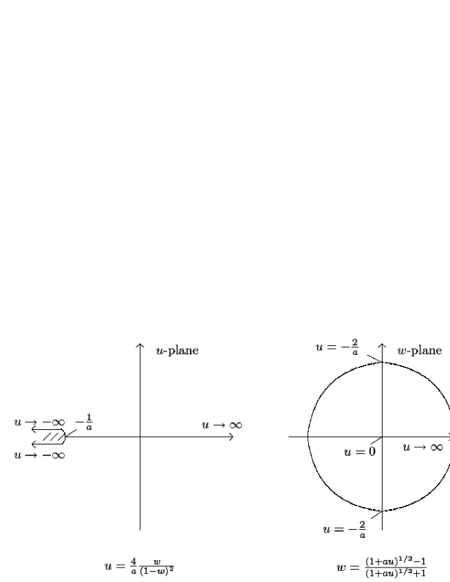
Figure 1: Conformal mapping of the cut-plane onto a disc. See the text for details.

In order to compute the integral in (12) on the whole real positive semi-axis one needs an analytic continuation of $B(t)$. It may be achieved by several methods. In particular, instead of the series of $B(t)$ its Padé-approximants can be used [39, 41, 42]. We prefer to use here a conformal mapping technique. In this method assuming that all the singularities of $B(u)$ lie on the negative real axis and that $B(u)$ is analytic in the whole complex plane excluding the cut from $-1/a$ to $-\infty$, one can perform in $B$ the change of variable $w(u)={\sqrt{1+a\,u}-1\over\sqrt{1+a\,u}+1}\Longleftrightarrow u(w)={4\over a}{w\over(1-w)^{2}}$, as it is shown in the figure 1. This change maps the complex $u$-plane cut from $u=-1/a$ to $-\infty$ onto the unit circle in the $w$-plane such that the singularities of $B(u)$ lying on the negative axis now lie on the boundary of the circle $|w|=1$. Then, the resulting expression of $B(w(u))$ has to be re-expanded in powers of $w(u)$. Finally, the resumed expression of the series $f$ writes:

$$f_{\mathrm{R}}(u)=\sum_{n}d_{n}(a,b)\int_{0}^{\infty}\rd t\,\,{\re^{-t}\,t^{b}\ \left[w(ut)\right]^{n}}\ ,$$ (13)

where $d_{n}(a,b)$ are the coefficients of the re-expansion of $B(u(w))$ in the powers of $w(u)$.

It is moreover interesting to generalize the above expression (13) in the following way [43]

$$f_{\mathrm{R}}(u)=\sum_{n}d_{n}(\alpha,a,b)\int_{0}^{\infty}\rd t\,\,{\re^{-t}\,t^{b}}\ {\left[w(ut)\right]^{n}\over\left[1-w(ut)\right]^{\alpha}}$$ (14)

since this allows to impose the strong coupling behavior of the series: $f(u\to\infty)\sim u^{\alpha/2}$.

If an infinite number of terms for $f(u)$ were known, expression (14) would be independent of the parameters $a$, $b$ and $\alpha$. However, once a truncation of the series is performed $f_{\mathrm{R}}(u)$ starts acquiring a dependence on these parameters. In principle, $a$ and $b$ are fixed by the large order behavior of the coefficients $a_{n}$ in series (9) [33], while $\alpha$ is determined by the strong coupling behavior of the initial series. However in many cases, only $a$ is known and $\alpha$ and $b$ must be considered either as free or variational parameters. In any case, the choice of values of $a$, $\alpha$ and $b$ must be validated a posteriori by checking that a small change of their values does not yield strong variations of the quantities under study.

The above described procedure may be generalized to the case of several variables. For instance, when $f$ is a function of two variables $u$ and $v$, the resummation technique used in [14] treats $f$ as a function of $u$ and of the ratio $z=v/u$:

$$f(u,z)=\sum_{n}a_{n}(z)\ u^{n}.$$ (15)

Then, keeping $z$ fixed and performing the resummation only in $u$ according to the steps (10)–(14), one gets:

$$f_{\mathrm{R}}(u,z)=\sum_{n}d_{n}(\alpha,a(z),b;z)\int_{0}^{\infty}\rd t\,\,{\re^{-t}\,t^{b}}{\left[w(ut;z)\right]^{n}\over\left[1-w(ut;z)\right]^{\alpha}}$$ (16)

with:

$$w(u;z)={\sqrt{1+a(z)\,u}-1\over\sqrt{1+a(z)\,u}+1}\$$ (17)

where, as above, the coefficients $d_{n}(\alpha,a(z),b,z)$ in (16) are computed so that the re-expansion of the right hand side of (16) in powers of $u$ coincides with that of (15).

2.2 Principles of convergence for results obtained with resummation

The dependence of the critical exponents upon the parameters $a,b$ and $\alpha$ is an indicator of the (non-) convergence of the perturbative series. Indeed, in principle, any converged physical quantity $Q$ should be independent of the choice of values of these parameters. However, in practice, at a given loop order ($L$), all calculated physical quantities depend (artificially) on them: $Q\to Q^{(L)}(a,b,\alpha)$. Fixing $a$ at the value obtained from the large order behavior, we consider that the optimal result for $Q$ at order $L$ corresponds to the values $(b_{\rm opt}^{(L)},\alpha_{\rm opt}^{(L)})$ of $(b,\alpha)$ for which Q depends the least on $b$ and $\alpha$, that is, for which it is stationary:

$$Q^{(L)}_{\rm opt}=Q^{(L)}(b_{\rm opt}^{(L)},\alpha_{\rm opt}^{(L)})\ \ \ \ \ \ {\rm with}\ \ \ \ \ \ \frac{\partial Q^{(L)}(b,\alpha)}{\partial b}\,{\bigg{|}_{b_{\rm opt}^{(L)},\alpha_{\rm opt}^{(L)}}}=\frac{\partial Q^{(L)}(b,\alpha)}{\partial\alpha}\,{\bigg{|}_{b_{\rm opt}^{(L)},\alpha_{\rm opt}^{(L)}}}=0\$$ (18)

where, of course, $b_{\rm opt}^{(L)}$ and $\alpha_{\rm opt}^{(L)}$ are functions of the order $L$. The validity of this procedure, known as the ‘‘Principle of Minimal Sensitivity’’ (PMS), requires that there is a unique pair $(b_{\rm opt}^{(L)},\alpha_{\rm opt}^{(L)})$ such that $Q^{(L)}$ is stationary. This is generically not the case: several stationary points are often found. A second principle allows us to ‘‘optimize’’ the results even in the case where there are several ‘‘optimal’’ values of $b$ and $\alpha$ at a given order $L$: this is the so-called ‘‘Principle of Fastest Apparent Convergence’’ (PFAC). The idea underlying this principle is that when the numerical value of $Q^{(L)}$ is almost converged (that is $L$ is sufficiently large to achieve a prescribed accuracy) then the next order of approximation must consist only in a small change of this value: $Q^{(L+1)}\simeq Q^{(L)}$. Thus, the preferred values of $b$ and $\alpha$ should be the ones for which the difference between two successive orders $Q^{(L+1)}(b^{(L+1)},\alpha^{(L+1)})-Q^{(L)}(b^{(L)},\alpha^{(L)})$ is minimal. In practice, the two principles should be used together for consistency and, if there are several solutions to equation (18) at order $L$ and/or $L+1$, one should choose the couples $(b_{\rm opt}^{(L)},\alpha_{\rm opt}^{(L)})$ and $(b_{\rm opt}^{(L+1)},\alpha_{\rm opt}^{(L+1)})$ for which the stationary values $Q^{(L)}(b_{\rm opt}^{(L)},\alpha_{\rm opt}^{(L)})$ and $Q^{(L+1)}(b_{\rm opt}^{(L+1)},\alpha_{\rm opt}^{(L+1)})$ are the closest, that is for which there is fastest apparent convergence. These principles have been developed and used in [33, 44, 23], see also [10].

3 $O(N)$-symmetric theory

Taking the above resummation procedure, let us show that it does not always eliminate unphysical FPs even in the simplest $\phi^{4}$ model in $d=3$. We study the $\beta_{u}$-function obtained within the massive scheme at four-, five- and six-loop orders [31]. As was noticed in [27], the non-resummed $\beta_{u}$-function has no non-trivial root at the even orders of perturbation theory. Applying the resummation procedure described by equations (9)–(14) we find the Wilson-Fisher FP P close to the origin (see figure 2). There exists a large amount of studies of FP P and its properties are well-known (see e. g. [2, 3, 5] and references therein). However, we also find for larger $u$, in addition to P and for some values of $\alpha$ and $b$, a new FP that we call S (in even orders of the loop expansion), see figure 2. Although this FP is unstable it changes the RG flow structure and, if taken seriously, it would correspond to a tricritical FP (1). However for the model under consideration the FP structure is well established [2] and this additional FP must be considered as an artifact of the fixed-$d$ approach.

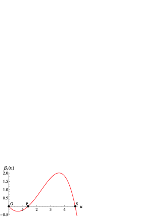
Figure 2: Resummed $\beta_{u}(u)$-function of the $O(4)$ model at $\alpha=6$ and $b=4$. The disks denote unstable FPs G and S, while the square corresponds to the stable FP P.

Let us compare the stability properties of the critical exponents defined at P and S. Here, we consider $\omega$ defined in equation (4), which is the leading correction to scaling exponent. We compute it at P and S from the resummed $\beta_{u}$-function and study its stability with the loop-order $L$ and with respect to variations of the resummation parameters $b$ and $\alpha$. Note that although the large order behavior of the series is known and leads to a preferred value of $a$ [45, 46] it is possible to take it as a free parameter and to also study the stability of all the results w.r.t. variations of this parameter. We choose here to fix $a$, then to vary $b$ and $\alpha$ so as to satisfy the PMS and PFAC and finally to check the stability of our results with respect to small variations of $a$.

3.1 Wilson-Fisher FP

First we consider $\omega$ for the Wilson-Fisher FP P. For $O(N)$ models, the analytically calculated value of $a$ is known to be $a=0.14777422\times 9/(N+8)$ [33] and we use it in our analysis.

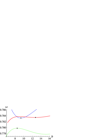
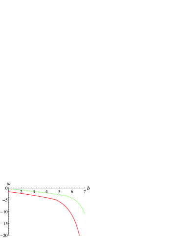
(a)

(b)

Figure 3: The exponent $\omega$ of the three-dimensional $O(4)$ model as a function of the resummation parameter $b$ calculated at (a) FP P and (b) FP S. Results for FP P are presented at four- (grey dashed curve (green online)), five- (dark dashed curve (blue online)) and six-loop (solid curve) orders. The dots at each loop-order correspond to a stationary value of $\omega=\omega(\alpha,b)$ in both $\alpha$ and $b$ directions at the same time ($L=4$: $\alpha=3.2$, $b=8.5$, $L=5$: $\alpha=5.2$, $b=9.5$, $L=6$: $\alpha=5$, $b=13$), at these values fastest apparent convergence between two successive loop orders is observed. Results for the FP S are presented in six and four loops at $\alpha=6$. No stationary point is found. The exponent $\omega$ is negative since S is repulsive.

The results of our calculations are shown in figure 3 (a) where the exponent $\omega$ for $N=4$ ($a=0.110831$) is shown as a function of the parameter $b$ for the values of $\alpha$ for which stationarity is found for both $b$ and $\alpha$. The values obtained for four-, five- and six-loop orders are very close. An indicator of the quality of the convergence is given by the difference between the fifth and the sixth orders: $\omega(L=6)-\omega(L=5)\simeq 2.10^{-4}$. Our six loop estimation is $\omega\simeq 0.783$. This result is compatible with the results obtained by Guida and Zinn-Justin [3] for $N=4$: $\omega=0.774\pm 0.020$ (fixed $d=3$, six/seven loops), $\omega=0.795\pm 0.030$ ($\epsilon$-expansion, five loops), which is a check of the reliability of both the resummation scheme and the convergence criteria used here.

3.2 Spurious FP

We now analyze $\omega$ at the FP $\bf S$. As expected, the results computed at $\bf S$ are very unstable with respect to variations of the parameters $\alpha$ and $b$. No stationary point is found for both $b$ and $\alpha$. To show the dependence of $\omega$ on $b$ at different loop orders we thus choose a given typical value of $\alpha$, see figure 3 (b). A monotonous decrease of $\omega$ while increasing $b$ is found. At fixed values of $\alpha$ and $b$ we moreover find that $|\omega|$ increases with the loop order.

At the end of this section some conclusion from the fixed $d=3$ analysis of the $O(N)$ model can be made. Our results for $\omega$ at P and S demonstrate two different features. For P, the convergence principles that we use — PMS and PFAC — allow us to find a reliable value of $\omega$, which is consistent with other estimations. On the contrary, $\omega$ at S does not show any stationarity when $b$ and $\alpha$ are varied. Furthermore, large differences between values in different loop orders (comparing to the results for FP P) are observed.

4 Cubic anisotropy

The previous section was devoted to the study of the $\phi^{4}$ model with one coupling. We now consider a more complicated model with two couplings, namely describing cubic anisotropy. The effective Hamiltonian for this model reads [6]:

$${\cal H}=\int\rd^{d}x\left\{{1\over 2}\left[(\partial\phi)^{2}+m_{0}^{2}\phi^{2}\right]+\frac{u_{0}}{4!}\left[\phi^{2}\right]^{2}+\frac{v_{0}}{4!}\sum_{i=1}^{N}\phi^{4}_{i}\right\}.$$ (19)

The Hamiltonian (19) is used to study the critical behavior of numerous magnetic and ferroelectric systems with appropriate order parameter symmetry (see e.g. [47]). The $\beta$-functions are known at six-loop order in the massive scheme [48]. Their FPs structure is known [6]. The FP $\bf G$ ($u^{*}=v^{*}=0$) and the Ising FP ($u^{*}=0,v^{*}\neq 0)$ are both unstable for all values of $N$. Two other FPs: the $O(N)$ symmetric FP P $(u^{*}\neq 0,v^{*}=0)$ and the mixed one $\bf M$ $(u^{*}\neq 0,v^{*}\neq 0)$ interchange their stability at a critical value $N_{\mathrm{c}}$ of $N$: for $N<N_{\mathrm{c}}$ the FP P is stable and $\bf M$ is unstable and vice versa for $N>{N_{\mathrm{c}}}$. The critical value ${N_{\mathrm{c}}}$ has been found to be slightly less than 3: for instance ${N_{\mathrm{c}}}=2.89\pm 0.04$ in [48] and ${N_{\mathrm{c}}}=2.862\pm 0.005$ in [47].

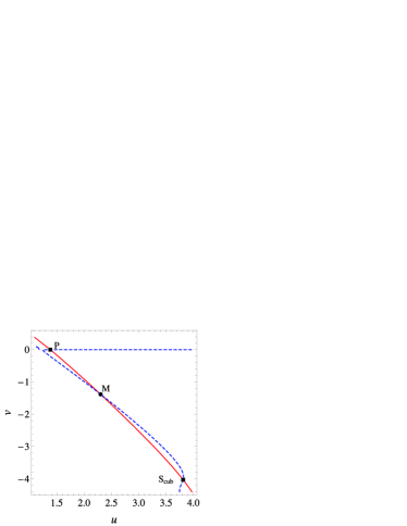
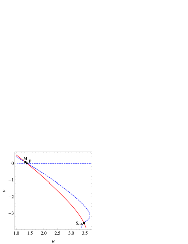
(a)

(b)

Figure 4: Lines of zeroes of $\beta_{u}$ (solid curves) and $\beta_{v}$ (dashed curves) for the cubic model for (a) $N=2$ with $\alpha=9$ and $b=9$ and (b) $N=3$ for $\alpha=8$ and $b=10$. The intersections of the solid and dashed lines correspond to different FPs: Wilson-Fisher P, cubic M and spurious S_cub. The discs correspond to unstable FPs, while squares denote stable FPs.

We have performed a stability analysis for the $N=2$, $N=3$ cases analogous to the $O(N)$ case. We take the $3d$ six-loop massive functions [48] and apply resummation procedure generalized to the case of two variables (15)–(17). Now, the FPs coordinates are defined by the system of equations:

$$\left\{\begin{array}[]{l}\beta_{u}(u,v)=0,\\ \\ \beta_{v}(u,v)=0.\end{array}\right.$$ (20)

Here, $\beta_{u}$ and $\beta_{v}$ stand for the resummed $\beta$-functions of the model defined by (19). Being functions of the two variables $u$ and $v$, $\beta_{u}$ and $\beta_{v}$ describe surfaces in the space $(u,v,\beta)$. The FPs correspond to the points of common intersections of these two surfaces with the $(u,v)$-plane. As a guide for the eyes, we plot the lines of zeroes of the resummed $\beta_{u}$ and $\beta_{v}$ functions. The FPs, if they exist, correspond to the crossing points of such lines. To obtain such curves, one must use definite values of the resummation parameters $a,\,b,\,\alpha$. As it has been shown in [12] the parameter $a$ for the cubic model (19) depends on the ratio $z=v/u$ and is: $a=0.14777422\times(9/(2N+8)+z)$ for $z>0$ and $a=0.14777422\times(9/(2N+8)+z/N)$ for $-{2N\over(N+1)}\times{9\over(N+8)}<z<0$. The resummed $\beta$-functions with the value $a$ above are depicted in figure 4 for $N=2$ and $N=3$.

From figure 4 one observes that, in addition to the usual FPs P and M, there exists another stable FP that has no counterpart within the $\varepsilon$-expansion for both values of $N$, denoted by us as S_cub. The presence of this FP, if taken seriously, would have important physical consequences since it would correspond to a second order phase transition with a new universality class. However no such transition has ever been reported. On the contrary, a first order behavior for all values of $N$ larger than ${N_{\mathrm{c}}}$ and $v_{0}<0$ is found within perturbative [48, 49] or non-perturbative [50] field theoretical analysis as well as numerical simulations [51] in related systems (four-state antiferromagnetic Potts model). Below we consider the dependence of physical quantities for the FP M and the spurious FP S_cub upon variations of the resummation parameters. We then compare the results obtained with those for the $O(N)$ model.

4.1 Mixed cubic FP

Since the cubic model involves two coupling constants $u$ and $v$ the stability of its FPs is defined by two exponents, $\omega_{1}$ and $\omega_{2}$, which are the generalizations of equation (4) for the case of two variables.

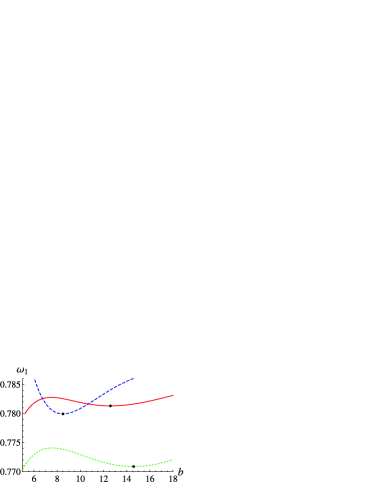
(a)

(b)

Figure 5: The exponent $\omega_{1}$ at the mixed FP M for $N=2$ (a) and $N=3$ (b) as a function of $b$ at four (grey dashed curves (green online)), five (dark dashed curves (blue online)) and six (solid curves) loops. The dots at each loop order correspond to a stationary value of $\omega=\omega(\alpha,b)$ in both $\alpha$ and $b$ directions at the same time. For $N=2$: $\alpha=3.4$, $b=14.3$ ($L=4$), $\alpha=5.7$, $b=8.3$ ($L=5$), $\alpha=5.8$, $b=13.4$ ($L=6$); for $N=3$: $\alpha=3.3$, $b=14.6$ ($L=4$), $\alpha=5.3$, $b=8.5$ ($L=5$), $\alpha=5.2$, $b=12.6$ ($L=6$). At these values fastest apparent convergence between two successive loop orders is observed.

At a stable FP, both $\omega_{1}$ and $\omega_{2}$ have positive real parts. Calculating these exponents for FP M (varying $\alpha$ and $b$ in different $L$) we observe a similar picture as the one obtained for $\omega$ computed at P in $O(N)$ models (which is intuitively expected). In figure 5 we only present the behavior of the larger exponent $\omega_{1}$ as function of the resummation parameter. Stationary points in $\alpha$ and $b$ are found. The values calculated at different loop orders at these points are very close to each other. For instance, for $N=3$ $\omega(L=6)-\omega(L=5)\approx 0.001$. Our six-loop results $\omega_{1}=0.781$, $\omega_{2}=0.011$ for $N=3$ agree with other six-loop estimates $\omega_{1}=0.781\pm 0.004$, $\omega_{2}=0.010\pm 0.004$ [48] and $\omega_{1}=0.777\pm 0.009$, $\omega_{2}=0.015\pm 0.002$ [47, 52].

4.2 Spurious cubic FP

We now study the FP S_cub. First, we note that S_cub for $N=2$ and $N=3$ is an attractive focus, that is $\omega_{1}$ and $\omega_{2}$ are complex conjugate and Re($\omega_{1}$)=Re($\omega_{2})>0$. Our results are shown in figure 6. The real part of $\omega_{i}$ does not show any stationary values as function of resummation parameters (see figure 6), and its behavior is similar to what was obtained for $\omega$ at S in the $O(N)$ model. Moreover, the difference of values obtained in successive loop orders is always more than 0.3, that is 300 times more than for the FP M. It is thus clear that S_cub is a spurious FP as is the FP S for the $O(N)$ model.

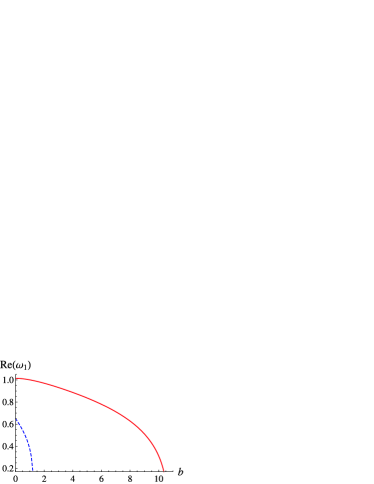
(a)

(b)

Figure 6: The real part of exponent $\omega_{1}$ in the frustrated FP for $N=2$ at $\alpha=5$ (a) and $N=3$ at $\alpha=6$ (b) as a function of $b$ at four (grey dashed curve (green online)), five (dark dashed curves (blue online)) and six (solid curves) loops.

5 Frustrated magnets

As in the previous section, we consider a model with two couplings but the one that describes frustrated antiferromagnets with non-collinear ordering. It is, for instance, used to describe a wide class of magnetic systems, such as antiferromagnets on stacked triangular lattice or helimagnets (see e.g. [9, 16]). Contrarily to the previously described cases the physics of the phase transition in this model is not yet settled. For $N=2$ and $3$, different approaches predict a first order transition [9] whereas it is found to be of second order in [12]. The study of this problem within minimal subtraction scheme [22, 23] already shed light on the reason of the discrepancy between these approaches showing that the stable FP should be considered spurious. We present here, within the massive RG scheme, additional arguments in this direction.

The effective Hamiltonian relevant for frustrated systems is given by:

$$\begin{array}[]{ll}\displaystyle{\mathcal{H}}{=}\int{\rm d^{d}}x\Bigg{\{}\frac{1}{2}\left[(\partial\phi_{1})^{2}{+}(\partial\phi_{2})^{2}+m^{2}(\phi_{1}^{2}{+}\phi_{2}^{2})\right]{+}\frac{u_{0}}{4!}\ \left[\phi_{1}^{2}{+}\phi_{2}^{2}\right]^{2}{+}\frac{v_{0}}{4!}\ \left[(\phi_{1}\cdot\phi_{2})^{2}{-}\phi_{1}^{2}\,\phi_{2}^{2}\right]\Bigg{\}}\end{array}$$ (21)

where the $\phi_{i}$, $i=1,2$, are $N$-component vector fields and $u_{0}$ and $v_{0}$ are bare couplings that satisfy $u_{0}>0$ and $v_{0}<4u_{0}$ – which corresponds to the region where the Hamiltonian is bounded from below. For $m^{2}>0$ the ground state of Hamiltonian (21) is given by $\phi_{1}=\phi_{2}=0$ while for $m^{2}<0$ it is given by a configuration where $\phi_{1}$ and $\phi_{2}$ are orthogonal with the same norm. The Hamiltonian (21) thus describes a symmetry breaking scheme between a disordered and an ordered phase where the $O(N)$ rotation group is broken down to $O(N-2)$ (for details see [9] for instance).

Let us first recall the picture of FPs obtained at leading order in $\varepsilon$ [16, 53, 54, 55]. The FPs have two coordinates, $u$ and $v$. For $N$ larger than a critical value $N_{\mathrm{c}}(d)$, four FPs exist: apart from the usual Gaussian ($u^{*}=v^{*}=0$) and $O(2N)$ ($u^{*}\neq 0,v^{*}=0$) FPs, one finds the chiral-antichiral pair of FPs with coordinates $u^{*}>0$ and $v^{*}>0$. The chiral FP C⁺ is stable, whereas the other one, antichiral FP C^-, is an unstable one. Above $N_{\mathrm{c}}(d)$, the transition is thus predicted to be of the second order for systems whose bare couplings lie in the basin of attraction of C⁺. When $N$ is lowered at fixed $d$, C⁺ and C^- become closer and closer and finally collide and disappear at $N=N_{\mathrm{c}}(d)$. Below $N_{\mathrm{c}}(d)$, there is no longer any stable FP and the transition is expected to be of first order. The value of $N_{\mathrm{c}}(d)$ for $d=3$ was a subject of intensive studies. In particular, it has been estimated within the $\varepsilon$-expansion [17, 18], within pseudo $\varepsilon$-expansion [11] and within a NPRG approach [9]. A six-loop estimate has found $N_{\mathrm{c}}=6.23\pm 0.21$ [11] within the pseudo-$\varepsilon$ expansion in good agreement with the value $N_{\mathrm{c}}=6.4\pm 0.4$ [56] derived from the resummed six-loops $\beta$-functions computed in $d=3$. According to this value of $N_{\mathrm{c}}$, the physical systems that correspond to $N=2$ or $N=3$ cannot undergo a second order phase transition. However a stable FP has been found for these values of $N$ in the fixed $d=3$ approach [12]. Since this FP is not found in the $\varepsilon$-expansion it is natural to wonder whether it is not an artifact of the fixed $d$ approach as it is the case for the FPs S and S_cub in the $O(N)$ and cubic model, respectively. Thus, below we reconsider the $\beta$-functions of the frustrated model (21) found in $d=3$ at six loops [12]. Our analysis concludes that the stable FP found for frustrated systems at $N=2,\,\,3$ [22, 23] is spurious.

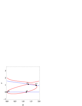
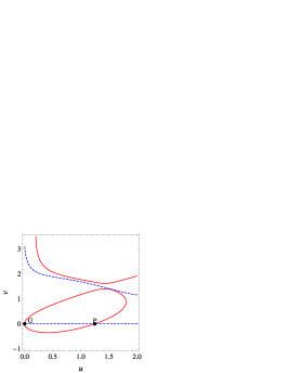
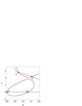
(a)

(b)

(c)

Figure 7: Lines of zeros of $\beta_{u}$ (solid curves) and $\beta_{v}$ (dashed curves) for $N=8$ (a), $N=6$ (b) and $N=4$ (c) [30]. Results are obtained at $\alpha=5$ and $b=15$. The crossings of solid and dashed lines correspond to different FPs: Gaussian (G), Wilson-Fisher (P), chiral (C⁺), antichiral (C^-) and spurious (S⁺, S^-).

First we investigate general situation with the change of $N$. Parameter $a$ for frustrated model has values depending on $N$ [12]: $a=0.14777422\times 9/(2N+8)$ for $4\frac{9}{(2N+8)}>z>0$ and $a=0.14777422\times(9/(2N+8)-z/2)$ for $z<0,\quad z>4\frac{9}{(2N+8)}$. Using this value in calculation we show the typical behavior (i.e. the behavior observed for the majority of $\alpha$, $b$) of the lines of zeros of resummed $\beta$-functions with fixed $d=3$ in figure 7 for different $N$, ranging from the large values of $N$, $N>N_{\mathrm{c}}$ (figure 7 (a) to the small ones, $N<N_{\mathrm{c}}$ (figure 7 (c). As one can see from the figures, the lines of zeros of $\beta_{u}$ form two branches, the upper and the lower one. Note that the lower branch has a form of a closed contour. This contour corresponds to zeros of function $\beta_{u}$ which exist already in the leading order in $\varepsilon$. For $N\geqslant 7$ a curve of zeros of $\beta_{v}$ intersects the closed contour generating the chiral-antichiral pair of FPs, C⁺ and C^- (see figure 7 (a)). When values of $N$ are between 7 and 6 this pair disappears in agreement with the scenario obtained in the $\varepsilon$-expansion and with an estimate $N_{\mathrm{c}}\approx 6.23$ [11]. Then, till $N\approx 5$ there is no intersection between curves of zeros $\beta_{u}$ and $\beta_{v}$ in the region $u>0$ and $v>0$ and therefore there are no FPs in the given region (see figure 7 (b)). While at $N<5$ we observe, that curve of zeros of $\beta_{v}$ intersects the upper branch of zeros of $\beta_{u}$ forming two FPs, stable S⁺ and unstable ones S^- (see figure 7 (c)). A similar situation has already been observed in [56] that has led to a conclusion concerning the existence of another critical value of $N$. From the above sketched analysis one can see that the FP solutions C⁺, C^-, on the one hand and S⁺, S^- on the other hand correspond to the crossing of different branches of the $\beta_{u}$ curve. In the first case (C⁺, C^-) this is the lower branch, whereas in the second case (S⁺, S^-) this is the upper one. Below, we will show the similarities in the behavior of solutions S⁺, S^- to those that were obtained in the former section 3 for the spurious FP. In the following subsections we separate the analysis of stable FPs for cases ‘‘large $N$’’ and ‘‘small $N$’’ meaning by this two different regimes when $N$ is greater than $N_{\mathrm{c}}$ (c.f. figure 7 (a)) or smaller than $N_{\mathrm{c}}$ (figure 7 (c)), correspondingly.

5.1 Case of large $N$

Similarly to the above analyzed cubic model here we present the results of the analysis for stability exponents at $d=3$. We start with the data obtained for the stable FP C⁺ at $N>N_{\mathrm{c}}$. In this case we take $N=8$, therefore $a=0.0554$, and analyze how the exponent $\omega$ changes with $\alpha$ and $b$. We find that the PMS is satisfied at four-, five- and six-loop orders: for suitable values of the parameters $b$ and $\alpha$ the two exponents $\omega_{1}$ and $\omega_{2}$ depend weakly on these parameters and are reasonably well converged. This is clear from figure 8, where we show the $b$-dependence of $\omega_{1}$ and $\omega_{2}$. Moreover, the difference between the values at five and six loops of, for instance, $\omega_{2}$ is small: $\omega_{2}(L=6)-\omega_{2}(L=5)\simeq 0.012$. Note that our values of $\omega_{1}$ and $\omega_{2}$ in this case are fully compatible with those obtained in [56].

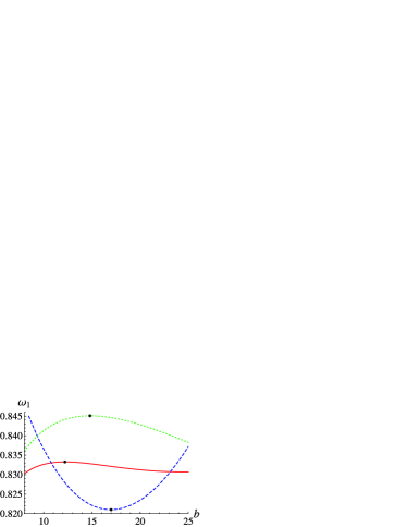
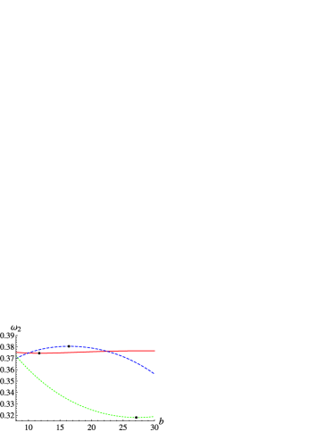
(a)

(b)

Figure 8: The exponents $\omega_{1}$(a) and $\omega_{2}$ (b) at FP of frustrated model for $N=8$ as a function of $b$ at four (grey dashed curves (green online)), five (dark dashed curves (blue online)) and six (solid curves) loops. The dots at each loop-order correspond to a stationary value of $\omega=\omega(\alpha,b)$ in both $\alpha$ and $b$ directions at the same time. For $\omega_{1}$: $\alpha=5.1$, $b=14.8$ ($L=4$), $\alpha=7.8$, $b=17$ ($L=5$), $\alpha=7$, $b=12.2$ ($L=6$); for $\omega_{2}$: $\alpha=6.5$, $b=27.1$ ($L=4$), $\alpha=7.9$, $b=16.4$ ($L=5$), $\alpha=7.5$, $b=11.7$ ($L=6$).

These results indicate that the convergence properties of the $N=8$ frustrated model are globally similar to those of the physical FPs of the $O(N)$ and cubic models although very likely less accurate because in the latter case the resummation is less efficient due to the presence of complex symmetry.

5.2 Case of small $N$

Now, let us study the peculiarities of the stable FP S⁺ in the region $u>0,\,v>0$ for the physical cases $N=2,\,3$. The results obtained at the calculation of $\omega$ at this FP with variations for $b$ and $\alpha$ are given in figure 9.

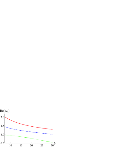
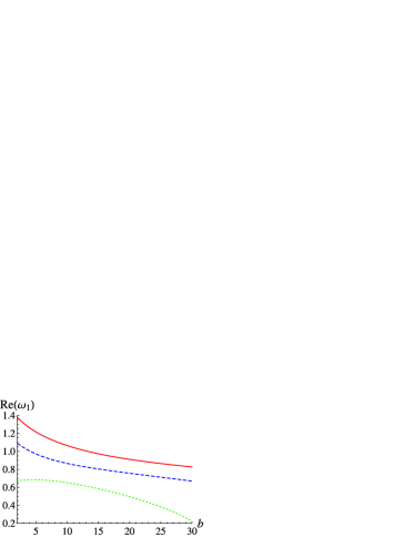
(a)

(b)

Figure 9: The real part of the exponent $\omega_{1}$ in the FP S⁺ for $N=2$ (a) and $N=3$ (b) as a function of $b$ for $\alpha=6$ at four (grey dashed curves (green online)), five (dark dashed curves (blue online)) and six (solid curves) loops.

As it was noted in [12], stability exponents attain (in most cases) complex values at FP S⁺ with positive real parts of $\omega$ indicating a stable focus topology. We, again, take for $a$ the value obtained from the large order analysis [12]: $a=0.1108$ for $N=2$ and $a=0.095$ for $N=3$. For these values of $a$ and for $L=4,5$ and $6$, we find that Re($\omega_{1}$) (or equivalently Re($\omega_{2}$)) considered as a function of $\alpha$ and $b$ is nowhere stationary, even approximately, see figure 9. Moreover, at fixed $\alpha$ and $b$, the gap between the values of Re($\omega_{1}$) at two successive loop-orders: Re($\omega_{1})(L+1)-$ Re($\omega_{1})(L)$, is always large, of order $0.5$ for $N=2$ and $0.2$ for $N=3$, see figure 9. Thus neither the PMS nor the PFAC are satisfied for these values of $N$.

The $b$-dependence of $\omega_{1}$ obtained in figure 9 shows the similarity with the results for the FP S of the $3d$ $O(N)$ model (compare with figure 3 (b)) as well as with S_cub of cubic model (compare with figure 6). From the figure 9 the bad convergence properties for spurious FP are evident. Also the value of $\omega$ in FP S⁺ decreases when increasing $b$, just as it was observed for the FP S and S_cub.

Thus we observe a situation analogous to the previously studied models. Similarly to the physical FPs of these models, for FP C⁺ at $N>N_{\mathrm{c}}$, we observe good convergent behavior, which is displayed via weak change of exponents and small difference between the results of different loop order. While for FP S⁺ at $N<N_{\mathrm{c}}$ we do not observe the regions of stabilization of critical exponents. The values of stability exponents considerably differ in different orders. Since such properties are characteristic of FP S and S_cub, this supports the unphysical character of FP S⁺.

6 Conclusions

The main motivation of the study reported in this paper was to attract attention to some problems that arise in the course of RG analysis of critical behavior of complex Hamiltonians. Being formulated briefly one can state that RG has proven its accuracy when it is used to calculate numerical values of different universal observables that govern the second order phase transition and critical behavior in more general sense. However, sometimes RG is used to prove the occurence of a critical point itself. In such cases, the occurence of stable and reachable FP of a RG transformation is considered to be the proof of a second order phase transition. This is the problem we addressed in our paper. Namely, given that in principle, a non-physical solution may arise in any computational scheme, how could one single-out such solutions from the physical ones?

In particular, several different solutions for FP may be obtained in the analysis of the expressions of $\beta$-functions obtained within the perturbative RG as series in coupling constant without use of $\varepsilon$- or pseudo-$\varepsilon$ expansions [27, 36] directly at fixed space dimension $d$. It is clear that the number of such solutions increases with an increase of the loop approximation. The way to distinguish between physical and unphysical FPs is resummation procedure, which is expected to eliminate all spurious solutions. However, generally this is not the case. As it follows from the analysis performed in this paper for the $O(N)$ model, except physical Wilson-Fisher FP, another FP survives. The current knowledge of the properties of $O(N)$ model at $d=3$ excludes the occurence of such FP. Additionally, the obtained FPs clearly differ in their convergent properties. In particular, the behavior of spurious FP is strongly dependent on the fit parameters used in resummation and does not satisfy the principles of convergence (PMS, PFAC). A completely identical picture is observed for the cubic model, whose critical behavior is also known. New (spurious) FP, found for this model by a fixed $d$ approach, demonstrates the same behavior as the spurious FP of $O(N)$ model.

Although the problem of discerning between physical and unphysical FPs is quite general. Here we address it taking as an example the phase transition for the model of frustrated magnets. The question of order of phase transition in such systems remains unclear. The experimental results make it possible to divide the conditionally tested materials into two groups that differ by their critical exponents. The feature of one group is negative exponent $\eta$, while the scaling relations are violated for the critical exponents of the other group (see review in [9]). Both phenomena should not occur at the second order phase transition. Recent numerical simulations give evidence of the first order phase transition for frustrated systems [57, 58, 59, 60, 61]. The RG investigations based on the $\varepsilon$- and pseudo-$\varepsilon$-expansions [16, 17, 11] indicate the absence of the second order phase transition within $\phi^{4}$ theory for a frustrated model at physical values $N=2$ and $N=3$. This was corroborated within NPRG [20, 19, 21, 9]. However, in the RG analysis at fixed $d$ with application of resummation procedures a stable FP was found at $N=2,\,\,3$, but only starting from four-loop approximation [12]. Since the topology of this FP is stable focus, the difference in the experimental data was explained by an approach of RG flows to this focus.

The properties of such FP were already checked within the minimal subtraction scheme [22, 23], which makes it possible to continuously follow the behavior of the FPs with the change of space dimension from $d=3$ to $d=4$, where only Gaussian FP describes the physics of a system. There, it was shown that the spurious FP found at $d=3$ persists at $d=4$ as well. Such an observation enabled us to assume that this FP is an unphysical one.

In the present study the expressions obtained in the massive scheme at $d=3$ are used. Therefore, it is impossible to trace them to $d=4$ by continuous change of $d$. However, the analysis we performed here shows that stable FPs obtained for values $N=2,\,\,3$ on the one hand and for the values higher than the critical value $N_{\mathrm{c}}$ one the other hand, differ in their behavior in respect to a variation of fit parameters of the resummation procedure. While for values of $N>N_{\mathrm{c}}$ reliable results may be chosen by principles of convergence, for $N<N_{\mathrm{c}}$ a strong dependence of FPs behavior on the resummation parameters does not make it possible to apply these principles. The latter fact serves as an argument to consider FPs for $N<N_{\mathrm{c}}$ to be unphysical ones.

Аналiз 3d масивних розвинень пертурбативної ренормалiзацiйної групи: делiкатна справа Б. Делямотlabel1, М. Дудкаlabel2, Ю. Головачlabel2,label3, Д. Муанаlabel1 label1 Лабораторiя теоретичної фiзики конденсованих середовищ, CNRS-UMR 7600, Унiверситет П’єра i Марiї Кюрi, 75252 Париж Cédex 05, Францiя label2 Iнститут фiзики конденсованих систем НАН України, UA–79011 Львiв, Україна label3 Iнститут теоретичної фiзики, Унiверситет Йогана Кеплера, A–4040 Лiнц, Австрiя

References

- [1] Wilson K.G., Kogut J., Phys. Rep., 1974, 12, 75.
- [2] Brézin E., Le Guillou J.C., Zinn-Justin J. – In: Domb C., Green M.S. (Eds.), Phase Transitions and Critical Phenomena, Vol. 6. Academic Press, London, 1976, p. 127; Amit D.J., Field Theory, the Renormalization Group, and Critical Phenomena. World Scientific, Singapore, 1989; Zinn-Justin J., Quantum Field Theory and Critical Phenomena. Oxford University Press, 1996; Kleinert H., Schulte-Frohlinde V., Critical Properties of -Theories. World Scientific, Singapore, 2001.
- [3] Guida R., Jinn-Justin J., J. Phys. A, 1998, 31, 8103.
- [4] de Gennes P.-G., Scaling Concepts in Polymer Physics. Cornell University Press, Ithaca, NY, 1979.
- [5] Pelissetto A., Vicari E., Phys. Rep., 2002, 368, 549.
- [6] Aharony A., Phys. Rev.B, 8, 1973, 4270; Aharony A. – In: Phase Transitions and Critical Phenomena, ed. by Domb C. and Lebowitz J. Academic Press, New York, 1976, Vol. 6, p. 357.
- [7] Folk R., Holovatch Yu., Yavors’kii T., Physics-Uspekhi, 2003, 46, 169 [Uspekhi Fizicheskikh Nauk, 2003, 173, 175]; Preprint arXiv: cond-mat/0106468.
- [8] Dudka M., Folk R., Holovatch Yu., J. Magn. Magn. Mater., 2005, 294, 305.
- [9] Delamotte B., Mouhanna D., Tissier M., Phys. Rev. B, 2004, 69, 134413.
- [10] Dudka M., Holovatch Yu., Yavors’kii T., J. Phys. A, 2004, 37, 1.
- [11] Holovatch Yu., Ivaneiko D., Delamotte B., J. Phys. A, 2004, 37, 3569.
- [12] Pelissetto A., Rossi P., Vicari E., Phys. Rev. B, 2001, 63, 140414.
- [13] Pelissetto A., Rossi P., Vicari E., Phys. Rev. B, 2001, 65, 020403.
- [14] Calabrese P., Parruccini P., Pelissetto A., Vicari E., Phys. Rev. B, 2004, 70, 174439.
- [15] Calabrese P., Parruccini P., Sokolov A.I., Phys. Rev. B, 2002, 66, 180403.
- [16] Kawamura H., Phys. Rev. B, 1988, 38, 4916.
- [17] Antonenko S.A., Sokolov A.I., Varnashev K.B., Phys. Lett. A, 1995, 208, 161.
- [18] Calabrese P., Parruccini P., Nucl. Phys. B, 2004, 679, 568.
- [19] Tissier M., Mouhanna D., Delamotte B., Phys. Rev. B, 2000, 61, 15327.
- [20] Tissier M., Delamotte B., Mouhanna D., Phys. Rev. Lett., 2000, 84, 5208.
- [21] Tissier M., Delamotte B., Mouhanna D., Phys. Rev. B, 2003, 67, 134422.
- [22] Delamotte B., Holovatch Yu, Ivaneyko D., Mouhanna D., Tissier M., Preprint arXiv: cond-mat/0609285.
- [23] Delamotte B., Holovatch Yu, Ivaneyko D., Mouhanna D., Tissier M., J. Stat. Mech., 2008, P03014.
- [24] Delamotte B., Dudka M., Holovatch Yu, Mouhanna D., Phys. Rev. B, 2010, 82, 104432; Preprint arXiv: 1009.1492.
- [25] Pelissetto A., Rossi P., Vicari E., Phys.Rev. B, 2001, 63, 140414; Pelissetto A,. Rossi P., Vicari E., Preprint arXiv: cond-mat/0007389.
- [26] ’t Hooft G., Veltman M. Nucl. Phys. B, 1972, 44, 189; ’t Hooft G., Nucl. Phys. B, 1973, 61, 455.
- [27] Parisi G., In: Proceedings of the Cargrése Summer Scool, 1973 unpublished; Parisi G., J. Stat. Phys, 1980, 23, 49.
- [28] Wilson K.G., Fisher M.E., Phys. Rev. Lett., 1972, 28, 240.
- [29] Kleinert H., Neu J., Schulte-Frohlinde V., Chetyrkin K.G., Larin S.A. Phys. Lett. B, 1991, 272, 39; Erratum: Phys. Lett. B, 1993, 319, 545.
- [30] Here and below we use the normalization of couplings and -functions in which the coefficient of the one-loop contribution in -functions equals -1
- [31] Antonenko S.A. and Sokolov A.I., Phys. Rev E, 1995, 51, 1894.
- [32] Nickel B.G. (unpublished) see Ref. 19 in [33].
- [33] Le Guillou J.C. and Zinn-Justin J., Phys. Rev. B, 1980, 21, 3976.
- [34] Kenna R., Lang C.B., Nucl. Phys. B, 1993, 393, 461.
- [35] Suslov I.M., Preprint arXiv: 0806.0789.
- [36] Schloms R., Dohm V., Europhys. Lett., 1987, 3, 413; Schloms R., Dohm V., Nucl. Phys. B, 1989, 328, 639.
- [37] We omit the case of one-loop degenerated -functions, as in the diluted Ising model. In such cases the two loop contibutios should be taken into account and Wilson-Fisher FP is found in the powers of . See e.g. [7]
- [38] Hardy G.H., Divergent Series, Oxford, 1948.
- [39] Baker G.A., Nickel B.G., Green M.S. and Meiron D.I., Phys. Rev. Lett., 1976, 36, 1351; Baker G.A., Nickel B.G., Meiron D.I., Phys. Rev. B, 1978, 17, 1365.
- [40] Holovatch Yu., Shpot M., J. Stat. Phys., 1992, 66, 867; Holovatch Yu., Krokhmal’s’kii T., J. Math. Phys., 1994, 35, 3866; Holovatch Yu. and Yavors’kii T., J. Stat. Phys., 1998, 93, 785; Shpot M., Condens. Matter Phys., 2010, 13, 13101.
- [41] Baker G.A., Jr., Graves-Morris P.R., Padé Approximants, Cambridge Univ. Press, New York, 1996.
- [42] Holovatch Yu., Blavats’ka V., Dudka M., Ferber C. V., Folk R., Yavors’kii T., Int. J. Mod. Phys. B, 2002, 16, 4027.
- [43] Kazakov D.I., Tarasov O.V., Shirkov D.V., Theor. Math. Phys., 1979, 38, 15.
- [44] Mudrov A.I., Varnashev K.B., Phys. Rev. E, 1998, 58, 5371.
- [45] Lipatov L.N. Zh.Éksp. Teor. Fiz., 1977, 72, 411. [ Sov. Phys. JETP, 1977, 45, 216].
- [46] Brézin E., Le Guillou J.C., Zinn-Justin J., Phys. Rev. D, 1977, 15, 1544; Phys. Rev. D, 1977, 15, 1558.
- [47] Folk R., Holovatch Yu. and Yavors’kii T., Phys. Rev. B, 2000, 62, 12195; Erratum: ibid. 2001, 63, 189901.
- [48] Carmona J.M., Pelissetto A., Vicari E., Phys. Rev. B, 2000, 61, 15136.
- [49] Calabrese P., Pelissetto A., Vicari E., Phys. Rev. B, 2003, 67, 024418.
- [50] Tissier M., Mouhanna D., Vidal J., Delamotte B., Phys. Rev. B, 2002, 65, 140402.
- [51] Itakura M., Phys. Rev. B, 1999, 60, 6558.
- [52] Value of is reported in the erratum [47] as smallest stability exponent, while value for largest is in the main reference [47].
- [53] Garel T., Pfeuty P., J. Phys. C: Solid St. Phys., 1976 , 9, L245.
- [54] Bailin D., Love A., Moore M.A., J. Phys. C: Solid State Phys., 1977, 10, 1159.
- [55] Yosefin M., Domany E., Phys. Rev. B, 1985, 32, 1778.
- [56] Calabrese P., Parruccini P., Sokolov A.I., Phys. Rev. B, 2003, 68, 094415.
- [57] Itakura M., J. Phys. Soc. Jap., 2003, 72, 74.
- [58] Peles A., Southern B.W., Delamotte B., Mouhanna D., Tissier M., Phys. Rev. B, 2004, 69, 220408(R).
- [59] Bekhechi S., Southern B.W., Peles A., Mouhanna D., Phys. Rev. E, 2006, 74, 016109.
- [60] Zelli M., Boese K., Southern B.W., Phys. Rev. B, 2007, 76, 224407.
- [61] Ngo V. Thanh, Diep H.T., Phys. Rev. E, 2008, 78, 031119; Ngo V. Thanh, Diep H.T., J. Appl. Phys., 2008, 103, No. 7, 07C712.