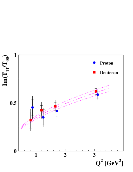
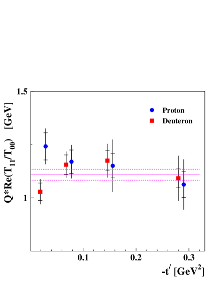
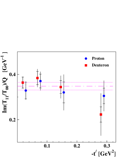
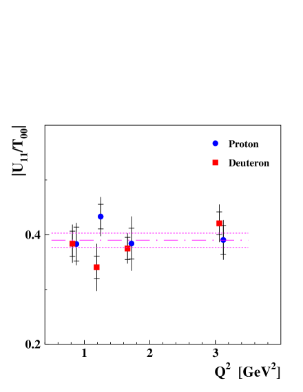
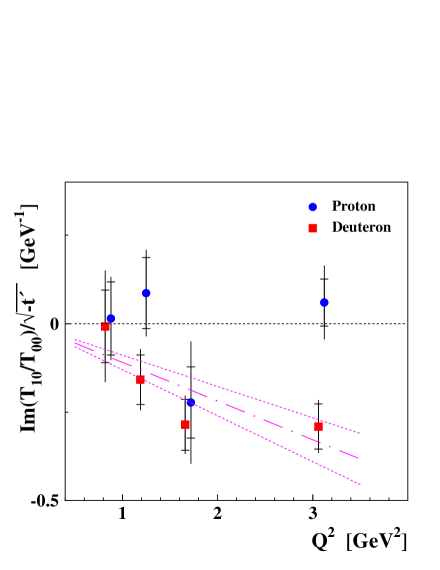
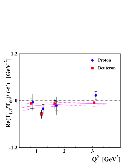
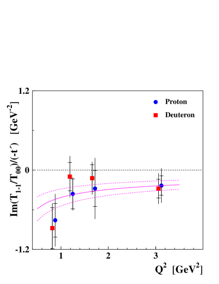
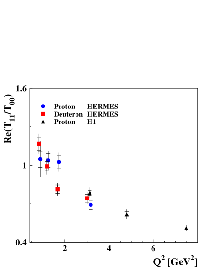
\hugehead
11institutetext: 1Physics Division, Argonne National Laboratory, Argonne, Illinois 60439-4843, USA
2Istituto Nazionale di Fisica Nucleare, Sezione di Bari, 70124 Bari, Italy
3School of Physics, Peking University, Beijing 100871, China
4Nuclear Physics Laboratory, University of Colorado, Boulder, Colorado 80309-0390, USA
5DESY, 22603 Hamburg, Germany
6DESY, 15738 Zeuthen, Germany
7Joint Institute for Nuclear Research, 141980 Dubna, Russia
8Physikalisches Institut, Universität Erlangen-Nürnberg, 91058 Erlangen, Germany
9Istituto Nazionale di Fisica Nucleare, Sezione di Ferrara and Dipartimento di Fisica, Università di Ferrara, 44100 Ferrara, Italy
10Istituto Nazionale di Fisica Nucleare, Laboratori Nazionali di Frascati, 00044 Frascati, Italy
11Department of Subatomic and Radiation Physics, University of Gent, 9000 Gent, Belgium
12Physikalisches Institut, Universität Gießen, 35392 Gießen, Germany
13SUPA, School of Physics and Astronomy, University of Glasgow, Glasgow G12 8QQ, United Kingdom
14Department of Physics, University of Illinois, Urbana, Illinois 61801-3080, USA
15Randall Laboratory of Physics, University of Michigan, Ann Arbor, Michigan 48109-1040, USA
16Lebedev Physical Institute, 117924 Moscow, Russia
17National Institute for Subatomic Physics (Nikhef), 1009 DB Amsterdam, The Netherlands
18Petersburg Nuclear Physics Institute, Gatchina, 188300 Leningrad region, Russia
19Institute for High Energy Physics, Protvino, 142281 Moscow region, Russia
20Institut für Theoretische Physik, Universität Regensburg, 93040 Regensburg, Germany
21Istituto Nazionale di Fisica Nucleare, Sezione Roma 1, Gruppo Sanità and Physics Laboratory, Istituto Superiore di Sanità, 00161 Roma, Italy
22TRIUMF, Vancouver, British Columbia V6T 2A3, Canada
23Department of Physics, Tokyo Institute of Technology, Tokyo 152, Japan
24Department of Physics and Astronomy, VU University, 1081 HV Amsterdam, The Netherlands
25Andrzej Soltan Institute for Nuclear Studies, 00-689 Warsaw, Poland
26Yerevan Physics Institute, 375036 Yerevan, Armenia

Ratios of Helicity Amplitudes for Exclusive ρ0superscript𝜌0\rho^{0} Electroproduction

The HERMES Collaboration
A. Airapetian
   12,15 N. Akopov    26 Z. Akopov    5 E.C. Aschenauer    6,111Now at: Brookhaven National Laboratory, Upton, New York 11772-5000, USA W. Augustyniak    25 R. Avakian    26 A. Avetissian    26 E. Avetisyan    5 S. Belostotski    18 N. Bianchi    10 H.P. Blok    17,24 A. Borissov    5,222Now at: Department of Physics and Astronomy 666 W.Hancock, Wayne State University, Detroit MI 48201, USA J. Bowles    13 V. Bryzgalov    19 J. Burns    13 M. Capiluppi    9 G.P. Capitani    10 E. Cisbani    21 G. Ciullo    9 M. Contalbrigo    9 P.F. Dalpiaz    9 W. Deconinck    5 R. De Leo    2 L. De Nardo    11,5 E. De Sanctis    10 M. Diefenthaler    14,8 P. Di Nezza    10 M. Düren    12 M. Ehrenfried    12 G. Elbakian    26 F. Ellinghaus    4 R. Fabbri    6 A. Fantoni    10 L. Felawka    22 S. Frullani    21 D. Gabbert    6 G. Gapienko    19 V. Gapienko    19 F. Garibaldi    21 G. Gavrilov    5,18,22 V. Gharibyan    26 F. Giordano    5,9 S. Gliske    15 M. Golembiovskaya    6 C. Hadjidakis    10 M. Hartig    5 D. Hasch    10 G. Hill    13 A. Hillenbrand    6 M. Hoek    13 Y. Holler    5 I. Hristova    6 Y. Imazu    23 A. Ivanilov    19 H.E. Jackson    1 H.S. Jo    11 S. Joosten    14 R. Kaiser    13,333Present address: International Atomic Energy Agency, A-1400 Vienna, Austria G. Karyan    26 T. Keri    12 E. Kinney    4 A. Kisselev    18 N. Kobayashi    23 V. Korotkov    19 V. Kozlov    16 P. Kravchenko    18 V.G. Krivokhijine    7 L. Lagamba    2 R. Lamb    14 L. Lapikás    17 I. Lehmann    13 P. Lenisa    9 L.A. Linden-Levy    14 A. López Ruiz    11 W. Lorenzon    15 X.-G. Lu    6 X.-R. Lu    23 B.-Q. Ma    3 D. Mahon    13 N.C.R. Makins    14 S.I. Manaenkov    18 L. Manfré    21 Y. Mao    3 B. Marianski    25 A. Martinez de la Ossa    4 H. Marukyan    26 C.A. Miller    22 Y. Miyachi    23 A. Movsisyan    26 V. Muccifora    10 M. Murray    13 A. Mussgiller    5,8 E. Nappi    2 Y. Naryshkin    18 A. Nass    8 M. Negodaev    6 W.-D. Nowak    6 L.L. Pappalardo    9 R. Perez-Benito    12 N. Pickert    8 P.E. Reimer    1 A.R. Reolon    10 C. Riedl    6 K. Rith    8 G. Rosner    13 A. Rostomyan    5 J. Rubin    14 D. Ryckbosch    11 Y. Salomatin    19 F. Sanftl    20 A. Schäfer    20 G. Schnell    6,11 K.P. Schüler    5 B. Seitz    13 T.-A. Shibata    23 V. Shutov    7 M. Stancari    9 M. Statera    9 E. Steffens    8 J.J.M. Steijger    17 F. Stinzing    8 S. Taroian    26 A. Terkulov    16 A. Trzcinski    25 M. Tytgat    11 A. Vandenbroucke    11 Y. Van Haarlem    11 C. Van Hulse    11 D. Veretennikov    18 V. Vikhrov    18 I. Vilardi    2 S. Wang    3 S. Yaschenko    6,8 S. Yen    22 W. Yu    12 B. Zihlmann    5 P. Zupranski25
(Received: / Revised version:)
Abstract

Exclusive ρ0superscript𝜌0\rho^{0}-meson electroproduction is studied in the HERMES experiment, using a 27.627.627.6 GeV longitudinally polarized electron/positron beam and unpolarized hydrogen and deuterium targets in the kinematic region 0.50.50.5 GeV<2Q2<7.0{}^{2}<Q^{2}<7.0 GeV2, 3.03.03.0 GeV <W<6.3absent𝑊6.3<W<6.3 GeV, and t<0.4superscript𝑡0.4-t^{\prime}<0.4 GeV2. Real and imaginary parts of the ratios of the natural-parity-exchange helicity amplitudes T11subscript𝑇11T_{11} (γTρTsubscriptsuperscript𝛾𝑇subscript𝜌𝑇\gamma^{*}_{T}\rightarrow\rho_{T}), T01subscript𝑇01T_{01} (γTρLsubscriptsuperscript𝛾𝑇subscript𝜌𝐿\gamma^{*}_{T}\rightarrow\rho_{L}), T10subscript𝑇10T_{10} (γLρTsubscriptsuperscript𝛾𝐿subscript𝜌𝑇\gamma^{*}_{L}\rightarrow\rho_{T}), and T11subscript𝑇11T_{1-1} (γTρTsubscriptsuperscript𝛾𝑇subscript𝜌𝑇\gamma^{*}_{-T}\rightarrow\rho_{T}) to T00subscript𝑇00T_{00} (γLρLsubscriptsuperscript𝛾𝐿subscript𝜌𝐿\gamma^{*}_{L}\rightarrow\rho_{L}) are extracted from the data. For the unnatural-parity-exchange amplitude U11subscript𝑈11U_{11}, the ratio |U11/T00|subscript𝑈11subscript𝑇00|U_{11}/T_{00}| is obtained. The Q2superscript𝑄2Q^{2} and tsuperscript𝑡t^{\prime} dependences of these ratios are presented and compared with perturbative QCD predictions.

1 Introduction

Exclusive electroproduction of vector mesons, e+Ne+V+N𝑒𝑁superscript𝑒𝑉superscript𝑁e+N\rightarrow e^{\prime}+V+N^{\prime}, has been the focus of investigation for decades. Not only is the reaction mechanism of intrinsic interest, but this process also offers the possibility of studying, in a model-dependent way, the structure of hadrons involved in the process Bauer ; INS . Using the one-photon-exchange approximation, all the measurable observables in electroproduction can be expressed in terms of the virtual photon spin-density matrix and the helicity amplitudes FλVλNλγλNsubscript𝐹subscript𝜆𝑉subscriptsuperscript𝜆𝑁subscript𝜆𝛾subscript𝜆𝑁F_{\lambda_{V}\lambda^{\prime}_{N}\lambda_{\gamma}\lambda_{N}} of the process

γ(λγ)+N(λN)V(λV)+N(λN).superscript𝛾subscript𝜆𝛾𝑁subscript𝜆𝑁𝑉subscript𝜆𝑉superscript𝑁subscriptsuperscript𝜆𝑁\gamma^{*}(\lambda_{\gamma})+N(\lambda_{N})\rightarrow V(\lambda_{V})+N^{\prime}(\lambda^{\prime}_{N})\;. (1)

Here, γsuperscript𝛾\gamma^{*} denotes the virtual photon exchanged between the lepton and the target nucleon, V𝑉V denotes the produced vector meson, and N(N)𝑁superscript𝑁N(N^{\prime}) the initial (final) nucleon. The helicities of the particles are given in parentheses in Eq. (1). The helicity amplitudes are defined in the virtual-photon-nucleon center-of-mass (CM) system. In order to make the discussion of the transition γVsuperscript𝛾𝑉\gamma^{*}\rightarrow V more transparent, we shall henceforth often omit the nucleon helicity indices using the notation FλVλγsubscript𝐹subscript𝜆𝑉subscript𝜆𝛾F_{\lambda_{V}\lambda_{\gamma}} instead of FλVλNλγλNsubscript𝐹subscript𝜆𝑉subscriptsuperscript𝜆𝑁subscript𝜆𝛾subscript𝜆𝑁F_{\lambda_{V}\lambda^{\prime}_{N}\lambda_{\gamma}\lambda_{N}}. The properties of helicity amplitudes can be studied in detail because the spin-density matrix of the virtual photon is well known from quantum electrodynamics and the spin-density matrix of the produced vector meson is experimentally accessible.

For unpolarized targets, the formalism of the spin-density matrix elements (SDMEs) of the produced vector meson was first presented in Ref. SW , where expressions of SDMEs in terms of helicity amplitudes were established. The formalism was then extended to the case of polarized targets in Ref. Fraas . Recently, a new general formalism for the description of the process in Eq. (1) through SDMEs was presented in Ref. Diehl .

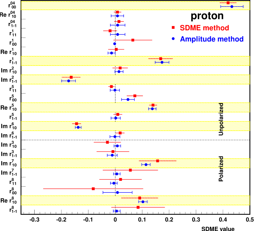
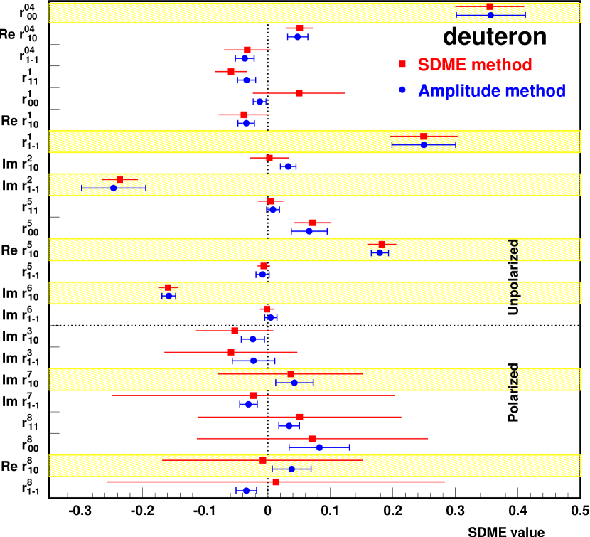
In order to determine SDMEs from experimental data, the SDMEs are considered as being independent free parameters in the fitting of the production and decay angular distribution of the vector meson. This is referred to as the “SDME method” in the rest of this work.

SDMEs are dimensionless quantities and therefore depend on ratios of amplitudes rather than on amplitudes themselves. The exact expressions for SDMEs given in Refs. SW ; Fraas ; Diehl can be rewritten in terms of amplitude ratios. In an alternative method of fitting the angular distribution, these ratios are considered as being independent free parameters. This method is referred to as the “amplitude method” in the rest of this work.

In order to extract the helicity amplitudes themselves, experimental data on the differential cross section with respect to the Mandelstam t𝑡t variable, dσ/dt𝑑𝜎𝑑𝑡d\sigma/dt (which is proportional to the sum of squared moduli of all the amplitudes) are required in addition to the experimentally determined amplitude ratios. An analysis of these combined data would allow the extraction of the moduli of all amplitudes and of the phase differences between them with the common phase remaining undetermined. However, the requisite information on nucleon spin-flip amplitudes is not available for data taken with unpolarized targets.

Exclusive meson production in hard lepton scattering has been shown to offer the possibility of constraining generalized parton distributions (GPDs), which provide correlated information on transverse spatial and longitudinal momentum distributions of partons in the nucleon gpd1 ; gpd2 ; gpd3 ; MD ; BR ; golos1 ; golos2 ; golos3 ; VGG ; GPV ; GPRV . Vector-meson production amplitudes contain various linear combinations of process-independent GPDs for quarks of various flavors and gluons. Access to GPDs relies on the factorization property of the process amplitude, i.e., the amplitude can be written as convolution of “non-perturbative” GPDs with amplitudes of hard partonic subprocesses calculated within the framework of perturbative quantum chromodynamics (pQCD) and quantum electrodynamics.

The amplitudes F0120±12subscript𝐹plus-or-minus012012F_{0\frac{1}{2}0\pm\frac{1}{2}} are the most interesting because, only for these and quantities constructed from them, was factorization proven strikman . Factorization is not proven for the other amplitudes nor for SDMEs, which depend on all helicity amplitudes. The amplitudes F0120±12subscript𝐹plus-or-minus012012F_{0\frac{1}{2}0\pm\frac{1}{2}} correspond to the transition of a longitudinally polarized (L) virtual photon to a longitudinally polarized vector meson, γLVLsubscriptsuperscript𝛾𝐿subscript𝑉𝐿\gamma^{*}_{L}\to V_{L}, and dominate at large photon virtuality Q2superscript𝑄2Q^{2}. Nevertheless, an application of the “modified perturbative approach” golos2 ; golos3 assumes that the factorization property also holds for the amplitudes F11subscript𝐹11F_{11} and F01subscript𝐹01F_{01}. The agreement found between certain calculated SDMEs and those extracted from HERMES DC-24 , ZEUS ZEUS2 , and H1 H1-amp data supports this assumption. The differential and total cross sections for longitudinal ρ0superscript𝜌0\rho^{0}-meson production by longitudinal photons are reasonably well described in the GPD-based approach of Refs. golos1 ; golos2 ; VGG ; GPV ; GPRV not only at the high energies of the HERA collider experiments ZEUS3 ; ZEUS4 ; H1-1 ; H1 ; H1-2 but also at intermediate energies covered by the fixed-target experiments E665 E665 , HERMES rho-xsec , and CLAS CLAS1 ; CLAS2 .

Amplitude ratios are useful not only as a tool for obtaining F00subscript𝐹00F_{00}. They can be used to study the general properties Diehl ; IK ; KNZ ; RK of the vector-meson-production amplitudes at very small and very large values of Q2superscript𝑄2Q^{2} and t𝑡t. They can also be used to test theoretical models. For these purposes, an amplitude ratio is more convenient than an SDME, which constitutes a more complicated object since any SDME depends on all the amplitude ratios. The amplitudes of the non-diagonal γVsuperscript𝛾𝑉\gamma^{*}\rightarrow V transitions F01subscript𝐹01F_{01} and F10subscript𝐹10F_{10} are known KNZ to be zero if any valence quark in the vector meson carries half of the longitudinal momentum of the meson in the infinite momentum frame. These amplitudes are the most sensitive objects for the study of the quark motion in vector mesons. The double-spin-flip amplitude F11subscript𝐹11F_{1-1} contains information on the gluon transversity generalized parton distribution MD ; BR ; IK ; KNZ ; RK ; Kivel in the nucleon, which cannot be obtained from inclusive deep-inelastic lepton-nucleon scattering.

Amplitude ratios in ρ0superscript𝜌0\rho^{0} and ϕitalic-ϕ\phi meson production on the proton were first studied by the H1 experiment H1-amp at the HERA collider. The results of the analysis of ρ0superscript𝜌0\rho^{0}-meson production at HERMES using the SDME method were published in Ref. DC-24 , where also the description of the HERMES spectrometer and details of the data treatment etc. can be found. The present work is a continuation of that analysis. In the analysis presented in this paper, ratios of helicity amplitudes to the amplitude F012012subscript𝐹012012F_{0\frac{1}{2}0\frac{1}{2}} are extracted separately for data taken with unpolarized hydrogen and deuterium targets first and then also for the combined datasets in a single analysis. A comparison of the proton and deuteron results allows the study of the degree of interference between I=1𝐼1I=1 exchanges of qq¯𝑞¯𝑞q\bar{q} pairs and I=0𝐼0I=0 exchanges of qq¯𝑞¯𝑞q\bar{q} pairs and two gluons.

2 Kinematics

In accordance with the notation of Ref. DC-24 , the kinematic variables of the process

eNeγNeρoNeπ+πN𝑒𝑁superscript𝑒superscript𝛾𝑁superscript𝑒superscript𝜌𝑜superscript𝑁superscript𝑒superscript𝜋superscript𝜋superscript𝑁eN\rightarrow e^{\prime}\gamma^{*}N\rightarrow e^{\prime}\rho^{o}N^{\prime}\rightarrow e^{\prime}\pi^{+}\pi^{-}N^{\prime} (2)

are defined as follows. The four-momenta of the incident and outgoing leptons are denoted by k𝑘k and ksuperscript𝑘k^{\prime}, the difference of which defines the four-momentum q=kk𝑞𝑘superscript𝑘q=k-k^{\prime} of the virtual photon γsuperscript𝛾\gamma^{*}. In the target rest frame (which is also called the laboratory or lab frame in this work), ϑitalic-ϑ\vartheta is the scattering angle between the incident and outgoing leptons, the energies of the leptons are denoted by E𝐸E and Esuperscript𝐸E^{\prime}.

Refer to caption
Figure 1: Definition of angles in the process eNeγNeρoNeπ+πN𝑒𝑁superscript𝑒superscript𝛾𝑁superscript𝑒superscript𝜌𝑜superscript𝑁superscript𝑒superscript𝜋superscript𝜋superscript𝑁eN\rightarrow e^{\prime}\gamma^{*}N\rightarrow e^{\prime}\rho^{o}N^{\prime}\rightarrow e^{\prime}\pi^{+}\pi^{-}N^{\prime}. Here ΦΦ\Phi is the angle between the ρ0superscript𝜌0\rho^{0} production plane and the lepton scattering plane in the CM system of virtual photon and target nucleon. See Ref. DESY2 for details. The variables θ𝜃\theta and ϕitalic-ϕ\phi are respectively the polar and azimuthal angles of the decay π+superscript𝜋\pi^{+} in the ρ0superscript𝜌0\rho^{0}-meson rest frame, with the Z𝑍Z axis being anti-parallel to the outgoing nucleon momentum.

The photon virtuality, given by

Q2=q2=(kk)2lab4EEsin2ϑ2,superscript𝑄2superscript𝑞2superscript𝑘superscript𝑘2superscript𝑙𝑎𝑏4𝐸superscript𝐸superscript2italic-ϑ2Q^{2}=-q^{2}=-(k-k^{\prime})^{2}\stackrel{{\scriptstyle lab}}{{\approx}}4\,E\,E^{\prime}\sin^{2}\frac{\vartheta}{2}, (3)

is positive in leptoproduction. In this equation, the electron rest mass is neglected. The four-momentum of the incident (recoiling) nucleon is denoted by p𝑝p (psuperscript𝑝p^{\prime}). The Bjorken scaling variable xBsubscript𝑥𝐵x_{B} is defined as

xB=Q22pq=Q22Mν,subscript𝑥𝐵superscript𝑄22𝑝𝑞superscript𝑄22𝑀𝜈x_{B}=\frac{Q^{2}}{2\,p\cdot q}=\frac{Q^{2}}{2\,M\,\nu}, (4)

with

ν=pqM=labEE,𝜈𝑝𝑞𝑀superscript𝑙𝑎𝑏𝐸superscript𝐸\nu=\frac{p\cdot q}{M}\stackrel{{\scriptstyle lab}}{{=}}E-E^{\prime}, (5)

so that ν𝜈\nu represents the energy transfer from the incoming lepton to the virtual photon in the laboratory frame. The squared invariant mass of the photon-nucleon system is given by

W2=(p+q)2=M2+2MνQ2.superscript𝑊2superscript𝑝𝑞2superscript𝑀22𝑀𝜈superscript𝑄2W^{2}=(p+q)^{2}=M^{2}+2\,M\,\nu-Q^{2}. (6)

The Mandelstam variable t𝑡t is defined by the relation

t=(qv)2,𝑡superscript𝑞𝑣2t=(q-v)^{2}, (7)

where v𝑣v is the four-momentum of the ρ0superscript𝜌0\rho^{0} meson being equal to pπ++pπsubscript𝑝superscript𝜋subscript𝑝superscript𝜋p_{\pi^{+}}+p_{\pi^{-}}, the sum of π+superscript𝜋\pi^{+} and πsuperscript𝜋\pi^{-} four-momenta. The variables t𝑡t, t0subscript𝑡0t_{0}, and t=tt0superscript𝑡𝑡subscript𝑡0t^{\prime}=t-t_{0} are always negative, where t0subscript𝑡0-t_{0} is the minimal value of t𝑡-t for given values of Q2superscript𝑄2Q^{2}, W𝑊W, and the ρ0superscript𝜌0\rho^{0}-meson mass MVsubscript𝑀𝑉M_{V}. At small values of tsuperscript𝑡-t^{\prime}, the approximation tvT2superscript𝑡superscriptsubscript𝑣𝑇2-t^{\prime}\approx v_{T}^{2} holds, where vTsubscript𝑣𝑇v_{T} is the transverse momentum of the ρ0superscript𝜌0\rho^{0} meson with respect to the direction of the virtual photon in the CM system.

The variable ϵitalic-ϵ\epsilon represents the ratio of fluxes of longitudinally and transversely polarized virtual photons and is given by

ϵ=1yQ24E21y+y22+Q24E2lab(1+2(1+ν2Q2)tan2ϑ2)1italic-ϵ1𝑦superscript𝑄24superscript𝐸21𝑦superscript𝑦22superscript𝑄24superscript𝐸2superscript𝑙𝑎𝑏superscript121superscript𝜈2superscript𝑄2superscript2italic-ϑ21\displaystyle\epsilon=\frac{1-y-\frac{Q^{2}}{4E^{2}}}{1-y+\frac{y^{2}}{2}+\frac{Q^{2}}{4E^{2}}}\!\!\stackrel{{\scriptstyle lab}}{{\approx}}\left(1+2\left(1+\frac{\nu^{2}}{Q^{2}}\right)\tan^{2}\frac{\vartheta}{2}\right)^{-1} (8)

with y=pq/pk=labν/E𝑦𝑝𝑞𝑝𝑘superscript𝑙𝑎𝑏𝜈𝐸y=p\cdot q/p\cdot k\stackrel{{\scriptstyle lab}}{{=}}\nu/E.

The “exclusivity” of ρ0superscript𝜌0\rho^{0} production in the process in Eq. (2) is characterized by the variable

ΔE=MX2M22M=labEV(Eπ++Eπ),Δ𝐸superscriptsubscript𝑀𝑋2superscript𝑀22𝑀superscript𝑙𝑎𝑏subscript𝐸𝑉subscript𝐸superscript𝜋subscript𝐸superscript𝜋\Delta E=\frac{M_{X}^{2}-M^{2}}{2M}\stackrel{{\scriptstyle lab}}{{=}}E_{V}-(E_{\pi^{+}}+E_{\pi^{-}}), (9)

where MX=(kk+ppπ+pπ)2subscript𝑀𝑋superscript𝑘superscript𝑘𝑝subscript𝑝superscript𝜋subscript𝑝superscript𝜋2M_{X}=\sqrt{(k-k^{\prime}+p-p_{\pi^{+}}-p_{\pi^{-}})^{2}} is the reconstructed invariant mass of the undetected hadronic system (missing mass), EV=ν+t/(2M)subscript𝐸𝑉𝜈𝑡2𝑀E_{V}=\nu+t/(2M) is the energy of the exclusively produced ρosuperscript𝜌𝑜\rho^{o} meson, and (Eπ++Eπ)subscript𝐸superscript𝜋subscript𝐸superscript𝜋(E_{\pi^{+}}+E_{\pi^{-}}) is the sum of the energies of the two detected pions in the laboratory system. For exclusive ρ0superscript𝜌0\rho^{0} electroproduction MX=Msubscript𝑀𝑋𝑀M_{X}=M and therefore ΔE=0Δ𝐸0\Delta E=0.

The angles used for the description of the process in Eq. (2) are defined according to Ref. DESY2 (see also Ref. DC-24 ) and presented in Fig. 1.

3 Formalism

3.1 Natural and Unnatural-Parity Exchange Helicity Amplitudes

In Ref. SW , exclusive ρ0superscript𝜌0\rho^{0}-meson leptoproduction is described by helicity amplitudes FλVλNλγλNsubscript𝐹subscript𝜆𝑉subscriptsuperscript𝜆𝑁subscript𝜆𝛾subscript𝜆𝑁F_{\lambda_{V}\lambda^{\prime}_{N}\lambda_{\gamma}\lambda_{N}} defined in the right-handed CM system of the virtual photon and target nucleon. In this system, the Z𝑍Z-axis is aligned along the virtual photon three-momentum q𝑞\vec{q} and the Y𝑌Y-axis is parallel to q×v𝑞𝑣\vec{q}\times\vec{v} where v𝑣\vec{v} is the ρ0superscript𝜌0\rho^{0} meson three-momentum as shown in Fig. 1. The helicity amplitude can be expressed as the scalar product of the matrix element of the electromagnetic current vector Jκsuperscript𝐽𝜅J^{\kappa} and the virtual-photon polarization vector eκ(λγ)superscriptsubscript𝑒𝜅subscript𝜆𝛾e_{\kappa}^{(\lambda_{\gamma})}

FλVλNλγλN=(1)λγvλVpλN|Jκ|pλNeκ(λγ),subscript𝐹subscript𝜆𝑉subscriptsuperscript𝜆𝑁subscript𝜆𝛾subscript𝜆𝑁superscript1subscript𝜆𝛾quantum-operator-product𝑣subscript𝜆𝑉superscript𝑝subscriptsuperscript𝜆𝑁superscript𝐽𝜅𝑝subscript𝜆𝑁superscriptsubscript𝑒𝜅subscript𝜆𝛾\displaystyle F_{\lambda_{V}\lambda^{\prime}_{N}\lambda_{\gamma}\lambda_{N}}=(-1)^{\lambda_{\gamma}}\langle v\lambda_{V}p^{\prime}\lambda^{\prime}_{N}|J^{\kappa}|p\lambda_{N}\rangle e_{\kappa}^{(\lambda_{\gamma})}, (10)

where a summation over the Lorentz index κ𝜅\kappa is performed. Here eκ(±1)superscriptsubscript𝑒𝜅plus-or-minus1e_{\kappa}^{(\pm 1)} and eκ(0)superscriptsubscript𝑒𝜅0e_{\kappa}^{(0)} indicate respectively transverse and longitudinal polarization of the virtual photon in the CM system:

e(±1)superscript𝑒plus-or-minus1\displaystyle e^{(\pm 1)} =\displaystyle= (e0,eX,eY,eZ)=(0,12,i2,0),subscript𝑒0subscript𝑒𝑋subscript𝑒𝑌subscript𝑒𝑍0minus-or-plus12𝑖20\displaystyle(e_{0},e_{X},e_{Y},e_{Z})=(0,\mp\frac{1}{\sqrt{2}},-\frac{i}{\sqrt{2}},0)\;, (11)
e(0)superscript𝑒0\displaystyle e^{(0)} =\displaystyle= 1Q(qZ,0,0,q0)1𝑄subscript𝑞𝑍00subscript𝑞0\displaystyle\frac{1}{Q}(q_{Z},0,0,q_{0}) (12)
=\displaystyle= 1WQ(Mν2+Q2,0,0,MνQ2).1𝑊𝑄𝑀superscript𝜈2superscript𝑄200𝑀𝜈superscript𝑄2\displaystyle\frac{1}{WQ}(M\sqrt{\nu^{2}+Q^{2}},0,0,M\nu-Q^{2})\;.

The ket vector |pλNket𝑝subscript𝜆𝑁|p\lambda_{N}\rangle corresponds to the initial nucleon and the bra vector vλVpλN|bra𝑣subscript𝜆𝑉superscript𝑝subscriptsuperscript𝜆𝑁\langle v\lambda_{V}p^{\prime}\lambda^{\prime}_{N}| represents the final state consisting of a ρ0superscript𝜌0\rho^{0} meson and the scattered nucleon.

Any helicity amplitude FλVλNλγλNsubscript𝐹subscript𝜆𝑉subscriptsuperscript𝜆𝑁subscript𝜆𝛾subscript𝜆𝑁F_{\lambda_{V}\lambda^{\prime}_{N}\lambda_{\gamma}\lambda_{N}} can be decomposed into the sum of an amplitude TλVλNλγλNsubscript𝑇subscript𝜆𝑉subscriptsuperscript𝜆𝑁subscript𝜆𝛾subscript𝜆𝑁T_{\lambda_{V}\lambda^{\prime}_{N}\lambda_{\gamma}\lambda_{N}} for natural-parity exchange (NPE) and an amplitude UλVλNλγλNsubscript𝑈subscript𝜆𝑉subscriptsuperscript𝜆𝑁subscript𝜆𝛾subscript𝜆𝑁U_{\lambda_{V}\lambda^{\prime}_{N}\lambda_{\gamma}\lambda_{N}} for unnatural-parity exchange (UPE) SW ; Fraas ; Diehl

FλVλNλγλN=TλVλNλγλN+UλVλNλγλN,subscript𝐹subscript𝜆𝑉subscriptsuperscript𝜆𝑁subscript𝜆𝛾subscript𝜆𝑁subscript𝑇subscript𝜆𝑉subscriptsuperscript𝜆𝑁subscript𝜆𝛾subscript𝜆𝑁subscript𝑈subscript𝜆𝑉subscriptsuperscript𝜆𝑁subscript𝜆𝛾subscript𝜆𝑁F_{\lambda_{V}\lambda^{\prime}_{N}\lambda_{\gamma}\lambda_{N}}=T_{\lambda_{V}\lambda^{\prime}_{N}\lambda_{\gamma}\lambda_{N}}+U_{\lambda_{V}\lambda^{\prime}_{N}\lambda_{\gamma}\lambda_{N}}, (13)

which obey the following symmetry relations

TλVλNλγλN=(1)λV+λγTλVλNλγλNsubscript𝑇subscript𝜆𝑉subscriptsuperscript𝜆𝑁subscript𝜆𝛾subscript𝜆𝑁superscript1subscript𝜆𝑉subscript𝜆𝛾subscript𝑇subscript𝜆𝑉subscriptsuperscript𝜆𝑁subscript𝜆𝛾subscript𝜆𝑁\displaystyle T_{\lambda_{V}\lambda^{\prime}_{N}\lambda_{\gamma}\lambda_{N}}=(-1)^{-\lambda_{V}+\lambda_{\gamma}}T_{-\lambda_{V}\lambda^{\prime}_{N}-\lambda_{\gamma}\lambda_{N}}
=(1)λNλNTλVλNλγλN,absentsuperscript1subscriptsuperscript𝜆𝑁subscript𝜆𝑁subscript𝑇subscript𝜆𝑉subscriptsuperscript𝜆𝑁subscript𝜆𝛾subscript𝜆𝑁\displaystyle=(-1)^{\lambda^{\prime}_{N}-\lambda_{N}}T_{\lambda_{V}-\lambda^{\prime}_{N}\lambda_{\gamma}-\lambda_{N}}, (14)
UλVλNλγλN=(1)λV+λγUλVλNλγλNsubscript𝑈subscript𝜆𝑉subscriptsuperscript𝜆𝑁subscript𝜆𝛾subscript𝜆𝑁superscript1subscript𝜆𝑉subscript𝜆𝛾subscript𝑈subscript𝜆𝑉subscriptsuperscript𝜆𝑁subscript𝜆𝛾subscript𝜆𝑁\displaystyle U_{\lambda_{V}\lambda^{\prime}_{N}\lambda_{\gamma}\lambda_{N}}=-(-1)^{-\lambda_{V}+\lambda_{\gamma}}U_{-\lambda_{V}\lambda^{\prime}_{N}-\lambda_{\gamma}\lambda_{N}}
=(1)λNλNUλVλNλγλN.absentsuperscript1subscriptsuperscript𝜆𝑁subscript𝜆𝑁subscript𝑈subscript𝜆𝑉subscriptsuperscript𝜆𝑁subscript𝜆𝛾subscript𝜆𝑁\displaystyle=-(-1)^{\lambda^{\prime}_{N}-\lambda_{N}}U_{\lambda_{V}-\lambda^{\prime}_{N}\lambda_{\gamma}-\lambda_{N}}\;. (15)

There are three important consequences of the symmetry relations (14) and (15SW ; Diehl :
i) The number of linearly independent NPE amplitudes is equal to 10 while only 8 independent UPE amplitudes describe the process in Eq. (1),
ii) No UPE amplitude exists for the transition γLρL0subscript𝛾𝐿subscriptsuperscript𝜌0𝐿\gamma_{L}\to\rho^{0}_{L}, so that in particular F012012T012012T00subscript𝐹012012subscript𝑇012012subscript𝑇00F_{0\frac{1}{2}0\frac{1}{2}}\equiv T_{0\frac{1}{2}0\frac{1}{2}}\equiv T_{00},
iii) For unpolarized targets there is no interference between NPE and UPE amplitudes SW ; Diehl .

In Regge phenomenology IW ; KS , an exchange of a single natural-parity reggeon [P=(1)J𝑃superscript1𝐽P=(-1)^{J} (pomeron, secondary reggeons ρ𝜌\rho, f2subscript𝑓2f_{2}, a2subscript𝑎2a_{2}, …)] contributes to the NPE amplitudes, while an exchange of a single unnatural-parity reggeon [P=(1)J𝑃superscript1𝐽P=-(-1)^{J} (π𝜋\pi, a1subscript𝑎1a_{1}, b1subscript𝑏1b_{1},…)] contributes to the UPE amplitudes CSM . It is worth noting that for a multi-reggeon-exchange contribution, there is no such one-to-one correspondence. For example, an exchange of two reggeons of “unnatural” parity contributes to the NPE amplitudes.

For convenience, we introduced in Ref. DC-24 the abbreviation ~12λNλN~12subscriptsubscriptsuperscript𝜆𝑁subscript𝜆𝑁\widetilde{\sum}\equiv\frac{1}{2}{\sum}_{\lambda^{\prime}_{N}\lambda_{N}} for the summation over the final nucleon helicity indices and for averaging over the initial spin states of the nucleon. For NPE amplitudes, transitions that are diagonal in nucleon helicity (λN=λNsubscriptsuperscript𝜆𝑁subscript𝜆𝑁\lambda^{\prime}_{N}=\lambda_{N}) are dominant. In this case, neglecting the small nucleon helicity-flip amplitudes TλV±12λγ12subscript𝑇minus-or-plusplus-or-minussubscript𝜆𝑉12subscript𝜆𝛾12T_{\lambda_{V}\pm\frac{1}{2}\lambda_{\gamma}\mp\frac{1}{2}} and using Eq. (14), the summation and averaging operation ~~\widetilde{\sum} reduces to one term:

~TλVλγTλVλγ~subscript𝑇subscript𝜆𝑉subscript𝜆𝛾subscriptsuperscript𝑇subscriptsuperscript𝜆𝑉subscriptsuperscript𝜆𝛾\displaystyle\widetilde{\sum}T_{\lambda_{V}\lambda_{\gamma}}T^{*}_{\lambda^{\prime}_{V}\lambda^{\prime}_{\gamma}} \displaystyle\equiv 12λNλNTλVλNλγλNTλVλNλγλN12subscriptsubscript𝜆𝑁subscriptsuperscript𝜆𝑁subscript𝑇subscript𝜆𝑉subscriptsuperscript𝜆𝑁subscript𝜆𝛾subscript𝜆𝑁subscriptsuperscript𝑇subscriptsuperscript𝜆𝑉subscriptsuperscript𝜆𝑁subscriptsuperscript𝜆𝛾subscript𝜆𝑁\displaystyle\frac{1}{2}\sum_{\lambda_{N}\lambda^{\prime}_{N}}T_{\lambda_{V}\lambda^{\prime}_{N}\lambda_{\gamma}\lambda_{N}}T^{*}_{\lambda^{\prime}_{V}\lambda^{\prime}_{N}\lambda^{\prime}_{\gamma}\lambda_{N}} (16)
=\displaystyle= TλV12λγ12TλV12λγ12+TλV12λγ12TλV12λγ12subscript𝑇subscript𝜆𝑉12subscript𝜆𝛾12subscriptsuperscript𝑇subscriptsuperscript𝜆𝑉12subscriptsuperscript𝜆𝛾12subscript𝑇subscript𝜆𝑉12subscript𝜆𝛾12subscriptsuperscript𝑇subscriptsuperscript𝜆𝑉12subscriptsuperscript𝜆𝛾12\displaystyle T_{\lambda_{V}\frac{1}{2}\lambda_{\gamma}\frac{1}{2}}T^{*}_{\lambda^{\prime}_{V}\frac{1}{2}\lambda^{\prime}_{\gamma}\frac{1}{2}}+T_{\lambda_{V}-\frac{1}{2}\lambda_{\gamma}\frac{1}{2}}T^{*}_{\lambda^{\prime}_{V}-\frac{1}{2}\lambda^{\prime}_{\gamma}\frac{1}{2}}
\displaystyle\approx TλV12λγ12TλV12λγ12TλVλγTλVλγ,subscript𝑇subscript𝜆𝑉12subscript𝜆𝛾12subscriptsuperscript𝑇subscriptsuperscript𝜆𝑉12subscriptsuperscript𝜆𝛾12subscript𝑇subscript𝜆𝑉subscript𝜆𝛾subscriptsuperscript𝑇subscriptsuperscript𝜆𝑉subscriptsuperscript𝜆𝛾\displaystyle T_{\lambda_{V}\frac{1}{2}\lambda_{\gamma}\frac{1}{2}}T^{*}_{\lambda^{\prime}_{V}\frac{1}{2}\lambda^{\prime}_{\gamma}\frac{1}{2}}\equiv T_{\lambda_{V}\lambda_{\gamma}}T^{*}_{\lambda^{\prime}_{V}\lambda^{\prime}_{\gamma}},

where TλVλNλγλNsubscriptsuperscript𝑇subscriptsuperscript𝜆𝑉subscriptsuperscript𝜆𝑁subscriptsuperscript𝜆𝛾subscript𝜆𝑁T^{*}_{\lambda^{\prime}_{V}\lambda^{\prime}_{N}\lambda^{\prime}_{\gamma}\lambda_{N}} represents the complex conjugate of the amplitude TλVλNλγλNsubscript𝑇subscriptsuperscript𝜆𝑉subscriptsuperscript𝜆𝑁subscriptsuperscript𝜆𝛾subscript𝜆𝑁T_{\lambda^{\prime}_{V}\lambda^{\prime}_{N}\lambda^{\prime}_{\gamma}\lambda_{N}}. Due to symmetry properties (see Eq. (14)), the abbreviated notation TλVλγsubscript𝑇subscript𝜆𝑉subscript𝜆𝛾T_{\lambda_{V}\lambda_{\gamma}} is used for the amplitudes TλV12λγ12=TλV12λγ12subscript𝑇subscript𝜆𝑉12subscript𝜆𝛾12subscript𝑇subscript𝜆𝑉12subscript𝜆𝛾12T_{\lambda_{V}\frac{1}{2}\lambda_{\gamma}\frac{1}{2}}=T_{\lambda_{V}-\frac{1}{2}\lambda_{\gamma}-\frac{1}{2}}.

In general, no dominance for UPE amplitudes can be proven either for diagonal transitions (λN=λNsubscript𝜆𝑁subscriptsuperscript𝜆𝑁\lambda_{N}=\lambda^{\prime}_{N}) or for transitions with nucleon helicity flip. Therefore, no relation analogous to Eq. (16) can be derived.

3.2 Spin Density Matrix Elements

The photon-spin-density matrix normalized to unit flux of transversely polarized virtual photons embodies the matrices ϱλγμγUsubscriptsuperscriptitalic-ϱ𝑈subscript𝜆𝛾subscript𝜇𝛾\varrho^{U}_{\lambda_{\gamma}\mu_{\gamma}} and ϱλγμγLsubscriptsuperscriptitalic-ϱ𝐿subscript𝜆𝛾subscript𝜇𝛾\varrho^{L}_{\lambda_{\gamma}\mu_{\gamma}} corresponding to unpolarized (U) and longitudinally (L) polarized lepton beams:

ϱλγμγU+L=ϱλγμγU+PBϱλγμγL,subscriptsuperscriptitalic-ϱ𝑈𝐿subscript𝜆𝛾subscript𝜇𝛾superscriptsubscriptitalic-ϱsubscript𝜆𝛾subscript𝜇𝛾𝑈subscript𝑃𝐵superscriptsubscriptitalic-ϱsubscript𝜆𝛾subscript𝜇𝛾𝐿\varrho^{U+L}_{\lambda_{\gamma}\mu_{\gamma}}=\varrho_{\lambda_{\gamma}\mu_{\gamma}}^{U}+P_{B}\;\varrho_{\lambda_{\gamma}\mu_{\gamma}}^{L}, (17)

where PBsubscript𝑃𝐵P_{B} is the longitudinal polarization of the lepton beam and ϱλγμγUsuperscriptsubscriptitalic-ϱsubscript𝜆𝛾subscript𝜇𝛾𝑈\varrho_{\lambda_{\gamma}\mu_{\gamma}}^{U} and ϱλγμγLsuperscriptsubscriptitalic-ϱsubscript𝜆𝛾subscript𝜇𝛾𝐿\varrho_{\lambda_{\gamma}\mu_{\gamma}}^{L} are defined in Ref. DC-24 . The spin density matrix ρλVμVsubscript𝜌subscript𝜆𝑉subscript𝜇𝑉\rho_{\lambda_{V}\mu_{V}} of the produced ρ0superscript𝜌0\rho^{0} meson is related to that of the virtual photon, ϱλγμγU+Lsubscriptsuperscriptitalic-ϱ𝑈𝐿subscript𝜆𝛾subscript𝜇𝛾\varrho^{U+L}_{\lambda_{\gamma}\mu_{\gamma}}, through the von Neumann formula SW :

ρλVμV=12𝒩λγμγλNλNFλVλNλγλNϱλγμγU+LFμVλNμγλN.subscript𝜌subscript𝜆𝑉subscript𝜇𝑉12𝒩subscriptsubscript𝜆𝛾subscript𝜇𝛾subscript𝜆𝑁subscriptsuperscript𝜆𝑁subscript𝐹subscript𝜆𝑉subscriptsuperscript𝜆𝑁subscript𝜆𝛾subscript𝜆𝑁subscriptsuperscriptitalic-ϱ𝑈𝐿subscript𝜆𝛾subscript𝜇𝛾superscriptsubscript𝐹subscript𝜇𝑉subscriptsuperscript𝜆𝑁subscript𝜇𝛾subscript𝜆𝑁\displaystyle\rho_{\lambda_{V}\mu_{V}}=\frac{1}{2{\mathcal{N}}}\sum_{\lambda_{\gamma}\mu_{\gamma}\lambda_{N}\lambda^{\prime}_{N}}\!\!\!\!\!\!\!\!F_{\lambda_{V}\lambda^{\prime}_{N}\lambda_{\gamma}\lambda_{N}}\;\varrho^{U+L}_{\lambda_{\gamma}\mu_{\gamma}}\;F_{\mu_{V}\lambda^{\prime}_{N}\mu_{\gamma}\lambda_{N}}^{*}.\hskip 11.38092pt (18)

Note that the phase factor (1)λγsuperscript1subscript𝜆𝛾(-1)^{\lambda_{\gamma}} in Eq. (10) is important for usual matrix summation over λγsubscript𝜆𝛾\lambda_{\gamma} and μγsubscript𝜇𝛾\mu_{\gamma} in Eq. (18). The normalization factor is given by

𝒩=𝒩T+ϵ𝒩L,𝒩subscript𝒩𝑇italic-ϵsubscript𝒩𝐿\displaystyle{\mathcal{N}}={\mathcal{N}}_{T}+\epsilon{\mathcal{N}}_{L}, (19)

with

𝒩Tsubscript𝒩𝑇\displaystyle{\mathcal{N}}_{T} =\displaystyle= ~(|T11|2+|T01|2+|T11|2\displaystyle\widetilde{\sum}\Big{(}|T_{11}|^{2}+|T_{01}|^{2}+|T_{1-1}|^{2} (20)
+|U11|2+|U01|2+|U11|2),\displaystyle+|U_{11}|^{2}+|U_{01}|^{2}+|U_{1-1}|^{2}\Big{)},
𝒩Lsubscript𝒩𝐿\displaystyle{\mathcal{N}}_{L} =\displaystyle= ~(|T00|2+2|T10|2+2|U10|2).~superscriptsubscript𝑇0022superscriptsubscript𝑇1022superscriptsubscript𝑈102\displaystyle\widetilde{\sum}\Big{(}|T_{00}|^{2}+2|T_{10}|^{2}+2|U_{10}|^{2}\Big{)}. (21)

Equation (21) is obtained by using the symmetry relations (14) and (15).

If the spin-density matrix of the virtual photon is decomposed into the standard set (see Ref. SW ) of nine hermitian matrices ΣηsuperscriptΣ𝜂\Sigma^{\eta} (η=0, 1,, 8𝜂018\eta=0,\;1,\;...,\;8), for the produced ρ0superscript𝜌0\rho^{0} meson a set of nine matrices rλVμVηsubscriptsuperscript𝑟𝜂subscript𝜆𝑉subscript𝜇𝑉r^{\eta}_{\lambda_{V}\mu_{V}} is obtained:

rλVμVη=12𝒩λγμγλNλNFλVλNλγλNΣλγμγηFμVλNμγλN.superscriptsubscript𝑟subscript𝜆𝑉subscript𝜇𝑉𝜂12𝒩subscriptsubscript𝜆𝛾subscript𝜇𝛾subscriptsuperscript𝜆𝑁subscript𝜆𝑁subscript𝐹subscript𝜆𝑉subscriptsuperscript𝜆𝑁subscript𝜆𝛾subscript𝜆𝑁superscriptsubscriptΣsubscript𝜆𝛾subscript𝜇𝛾𝜂superscriptsubscript𝐹subscript𝜇𝑉subscriptsuperscript𝜆𝑁subscript𝜇𝛾subscript𝜆𝑁\displaystyle r_{\lambda_{V}\mu_{V}}^{\eta}\!\!\!=\frac{1}{2{\mathcal{N}}}\!\!\!\sum_{\lambda_{\gamma}\mu_{\gamma}\lambda^{\prime}_{N}\lambda_{N}}\!\!\!\!\!\!\!\!\!F_{\lambda_{V}\lambda^{\prime}_{N}\lambda_{\gamma}\lambda_{N}}\Sigma_{\lambda_{\gamma}\mu_{\gamma}}^{\eta}F_{\mu_{V}\lambda^{\prime}_{N}\mu_{\gamma}\lambda_{N}}^{*}. (22)

If an experiment is performed at fixed beam energy, a (Rosenbluth rosenbluth ) decomposition into contributions from longitudinally and transversely polarized virtual photons is impossible. In this case, the contributions from the matrix elements rλVμV0superscriptsubscript𝑟subscript𝜆𝑉subscript𝜇𝑉0r_{\lambda_{V}\mu_{V}}^{0} and rλVμV4superscriptsubscript𝑟subscript𝜆𝑉subscript𝜇𝑉4r_{\lambda_{V}\mu_{V}}^{4} cannot be disentangled and the only measurable combination is

rλVμV04rλVμV0+ϵrλVμV4.subscriptsuperscript𝑟04subscript𝜆𝑉subscript𝜇𝑉subscriptsuperscript𝑟0subscript𝜆𝑉subscript𝜇𝑉italic-ϵsubscriptsuperscript𝑟4subscript𝜆𝑉subscript𝜇𝑉\displaystyle r^{04}_{\lambda_{V}\mu_{V}}\equiv r^{0}_{\lambda_{V}\mu_{V}}+\epsilon r^{4}_{\lambda_{V}\mu_{V}}\;. (23)

3.3 Three-dimensional Angular Distribution

The formula for the angular distribution of the scattered electrons/positrons and π+superscript𝜋\pi^{+} mesons from the decay ρ0π+πsuperscript𝜌0superscript𝜋superscript𝜋\rho^{0}\rightarrow\pi^{+}\pi^{-} for the case of a longitudinally polarized beam and an unpolarized target SW is given by

𝒲U+L(Φ,ϕ,cosθ)=superscript𝒲𝑈𝐿Φitalic-ϕ𝜃absent\displaystyle{\mathcal{W}}^{U+L}(\Phi,\phi,\cos{\theta})=
𝒲U(Φ,ϕ,cosθ)+PB𝒲L(Φ,ϕ,cosθ).superscript𝒲𝑈Φitalic-ϕ𝜃subscript𝑃𝐵superscript𝒲𝐿Φitalic-ϕ𝜃\displaystyle{\mathcal{W}}^{U}(\Phi,\phi,\cos{\theta})+P_{B}{\mathcal{W}}^{L}(\Phi,\phi,\cos{\theta})\;. (24)

Here 𝒲U(Φ,ϕ,cosθ)superscript𝒲𝑈Φitalic-ϕ𝜃\mathcal{W}^{U}(\Phi,\phi,\cos{\theta}) represents the angular distribution when both beam and target are unpolarized (see Eq. (25)) and 𝒲L(Φ,ϕ,cosθ)superscript𝒲𝐿Φitalic-ϕ𝜃\mathcal{W}^{L}(\Phi,\phi,\cos{\theta}) is the additional term arising for longitudinally polarized beam (see Eq. (26)).

𝒲U(Φ,ϕ,cosθ)superscript𝒲𝑈Φitalic-ϕ𝜃\displaystyle\mathcal{W}^{U}(\Phi,\phi,\cos{\theta}) =\displaystyle= 38π2[12(1r0004)+12(3r00041)cos2θ2Re{r1004}sin2θcosϕr1104sin2θcos2ϕ\displaystyle\frac{3}{8\pi^{2}}\Bigg{[}\frac{1}{2}(1-r^{04}_{00})+\frac{1}{2}(3r^{04}_{00}-1)\cos^{2}{\theta}-\sqrt{2}\mathrm{Re}\{r^{04}_{10}\}\sin 2\theta\cos\phi-r^{04}_{1-1}\sin^{2}\theta\cos 2\phi\hskip 28.45274pt (25)
\displaystyle- ϵcos2Φ(r111sin2θ+r001cos2θ2Re{r101}sin2θcosϕr111sin2θcos2ϕ)italic-ϵ2Φsubscriptsuperscript𝑟111superscript2𝜃subscriptsuperscript𝑟100superscript2𝜃2Resubscriptsuperscript𝑟1102𝜃italic-ϕsubscriptsuperscript𝑟111superscript2𝜃2italic-ϕ\displaystyle\epsilon\cos 2\Phi\Big{(}r^{1}_{11}\sin^{2}\theta+r^{1}_{00}\cos^{2}{\theta}-\sqrt{2}\mathrm{Re}\{r^{1}_{10}\}\sin 2\theta\cos\phi-r^{1}_{1-1}\sin^{2}\theta\cos 2\phi\Big{)}
\displaystyle- ϵsin2Φ(2Im{r102}sin2θsinϕ+Im{r112}sin2θsin2ϕ)italic-ϵ2Φ2Imsubscriptsuperscript𝑟2102𝜃italic-ϕImsubscriptsuperscript𝑟211superscript2𝜃2italic-ϕ\displaystyle\epsilon\sin 2\Phi\Big{(}\sqrt{2}\mathrm{Im}\{r^{2}_{10}\}\sin 2\theta\sin\phi+\mathrm{Im}\{r^{2}_{1-1}\}\sin^{2}\theta\sin 2\phi\Big{)}
+\displaystyle+ 2ϵ(1+ϵ)cosΦ(r115sin2θ+r005cos2θ2Re{r105}sin2θcosϕr115sin2θcos2ϕ)2italic-ϵ1italic-ϵΦsubscriptsuperscript𝑟511superscript2𝜃subscriptsuperscript𝑟500superscript2𝜃2Resubscriptsuperscript𝑟5102𝜃italic-ϕsubscriptsuperscript𝑟511superscript2𝜃2italic-ϕ\displaystyle\sqrt{2\epsilon(1+\epsilon)}\cos\Phi\Big{(}r^{5}_{11}\sin^{2}{\theta}+r^{5}_{00}\cos^{2}\theta-\sqrt{2}\mathrm{Re}\{r^{5}_{10}\}\sin 2\theta\cos\phi-r^{5}_{1-1}\sin^{2}\theta\cos 2\phi\Big{)}
+\displaystyle+ 2ϵ(1+ϵ)sinΦ(2Im{r106}sin2θsinϕ+Im{r116}sin2θsin2ϕ)],\displaystyle\sqrt{2\epsilon(1+\epsilon)}\sin\Phi\Big{(}\sqrt{2}\mathrm{Im}\{r^{6}_{10}\}\sin 2\theta\sin\phi+\mathrm{Im}\{r^{6}_{1-1}\}\sin^{2}\theta\sin 2\phi\Big{)}\Bigg{]},
𝒲L(Φ,ϕ,cosθ)superscript𝒲𝐿Φitalic-ϕ𝜃\displaystyle\mathcal{W}^{L}(\Phi,\phi,\cos\theta) =\displaystyle= 38π2[1ϵ2(2Im{r103}sin2θsinϕ+Im{r113}sin2θsin2ϕ)\displaystyle\frac{3}{8\pi^{2}}\Bigg{[}\sqrt{1-\epsilon^{2}}\Big{(}\sqrt{2}\mathrm{Im}\{r^{3}_{10}\}\sin 2\theta\sin\phi+\mathrm{Im}\{r^{3}_{1-1}\}\sin^{2}\theta\sin 2\phi\Big{)} (26)
+\displaystyle+ 2ϵ(1ϵ)cosΦ(2Im{r107}sin2θsinϕ+Im{r117}sin2θsin2ϕ)2italic-ϵ1italic-ϵΦ2Imsubscriptsuperscript𝑟7102𝜃italic-ϕImsubscriptsuperscript𝑟711superscript2𝜃2italic-ϕ\displaystyle\sqrt{2\epsilon(1-\epsilon)}\cos\Phi\Big{(}\sqrt{2}\mathrm{Im}\{r^{7}_{10}\}\sin 2\theta\sin\phi+\mathrm{Im}\{r^{7}_{1-1}\}\sin^{2}\theta\sin 2\phi\Big{)}
+\displaystyle+ 2ϵ(1ϵ)sinΦ(r118sin2θ+r008cos2θ2Re{r108}sin2θcosϕr118sin2θcos2ϕ)].\displaystyle\sqrt{2\epsilon(1-\epsilon)}\sin\Phi\Big{(}r^{8}_{11}\sin^{2}\theta+r^{8}_{00}\cos^{2}\theta-\sqrt{2}\mathrm{Re}\{r^{8}_{10}\}\sin 2\theta\cos\phi-r^{8}_{1-1}\sin^{2}\theta\cos 2\phi\Big{)}\Bigg{]}.

4 The Amplitude Method

4.1 Comparison of the SDME and Amplitude Methods

The SDME method for analyzing experimental data has the disadvantage that, in general, numerators of SDMEs depend on several ratios of helicity amplitudes (see Refs. SW ; DC-24 ) while the denominator common for all SDMEs depends on all the amplitude ratios. Therefore, if an SMDE extracted from data differs from model calculations, the source of the discrepancy is difficult to identify.

In total there are 18 independent amplitudes SW ; Fraas ; Diehl . Since SDMEs depend on ratios of these complex amplitudes to F00subscript𝐹00F_{00}, any SDME comprises 34 real, independent functions. However, the number of SDMEs to be extracted from experimental data in polarized particle scattering is larger. For instance, there are 47 SDMEs when both beam and target are longitudinally polarized, while the angular distribution for longitudinal beam polarization and transverse target polarization depends on 71 SDMEs Diehl . While the SDMEs can be completely expressed in terms of amplitude ratios, the fact that there are many more SDMEs than amplitude ratios implies that the SDMEs obey some relations. Due to the complicated inter-dependence on amplitude ratios, SDMEs cannot be considered as independent quantities and amplitude ratios can provide a more economical basis for fitting angular distributions of decay particles. This implies that the SDME values calculated from extracted amplitude ratios can be expected to be more accurate than those from direct SDME fits.

SDMEs calculated using the extracted helicity amplitude ratios may differ from those obtained with the SDME method. The SDMEs calculated from amplitude ratios are more constrained than those obtained by the SDME method. In general, any set of SDMEs obtained with the SDME method is physical only if it can be described in terms of amplitude ratios. Certain conditions, called positivity constraints, that must be satisfied by SDMEs in order to be expressed through amplitude ratios were considered in Ref. Diehl . However, the full set of conditions that must be satisfied by SDMEs in order to be expressible in terms of helicity amplitude ratios is currently unknown.

4.2 Hierarchy of Helicity Amplitudes

The number of amplitude ratios to be extracted from data can be reduced if there exists a hierarchy for the moduli of helicity amplitudes. For large photon virtuality Q2superscript𝑄2Q^{2} and small |t|superscript𝑡|t^{\prime}|, such a hierarchy among helicity amplitudes was predicted theoretically IK ; KNZ and confirmed experimentally H1 ; DC-24 ; ZEUS1 . According to this hierarchy, there are a few significant amplitudes while the contributions of other amplitudes may be neglected within the present experimental accuracy. In a given kinematic region, the hierarchy of the amplitudes is governed by one or more “small kinematic parameters” that determine the contribution of various amplitudes to the process.

4.2.1 s𝑠s-Channel Helicity Conservation

It was observed Bauer ; INS that, at small |t|superscript𝑡|t^{\prime}|, the amplitudes with a helicity flip in the transition γVsuperscript𝛾𝑉\gamma^{*}\to V (λVλγsubscript𝜆𝑉subscript𝜆𝛾\lambda_{V}\neq\lambda_{\gamma}) are much smaller than those for diagonal transitions where the helicity of the vector meson is equal to that of the virtual photon (λV=λγsubscript𝜆𝑉subscript𝜆𝛾\lambda_{V}=\lambda_{\gamma}). This behavior is controlled by the small parameter

α=tM,𝛼superscript𝑡𝑀\displaystyle\alpha=\frac{\sqrt{-t^{\prime}}}{M}, (27)

where M𝑀M is a typical hadronic mass, usually taken to be the nucleon mass. This dominance of the γVsuperscript𝛾𝑉\gamma^{*}\rightarrow V transition that is diagonal with respect to helicity is called the s𝑠s-channel helicity conservation (SCHC) approximation. Furthermore, it was shown MSI that for small |t|superscript𝑡|t^{\prime}| and Q2>2M2superscript𝑄22superscript𝑀2Q^{2}>2M^{2}, NPE amplitudes with nucleon helicity flip are suppressed compared to amplitudes describing diagonal transitions with λN=λNsubscript𝜆𝑁subscriptsuperscript𝜆𝑁\lambda_{N}=\lambda^{\prime}_{N}. The same small parameter given by Eq. (27) controls this suppression.

As only an unpolarized target is considered here, there is no linear contribution of nucleon-helicity-flip amplitudes to the relevant SDMEs SW ; Diehl . The fractional contribution of NPE amplitudes with nucleon helicity flip is suppressed by a factor α2superscript𝛼2\alpha^{2}, so that we need to consider only NPE amplitudes with λN=λNsubscript𝜆𝑁subscriptsuperscript𝜆𝑁\lambda_{N}=\lambda^{\prime}_{N} if we neglect terms of order α2superscript𝛼2\alpha^{2}.

The SCHC NPE amplitudes are T00subscript𝑇00T_{00} and T11subscript𝑇11T_{11}. The helicity-flip amplitudes T01subscript𝑇01T_{01} and T10subscript𝑇10T_{10} are proportional to the small factor α𝛼\alpha, while the double-helicity-flip amplitude T11subscript𝑇11T_{1-1} is proportional to α2superscript𝛼2\alpha^{2}.

4.2.2 Twist decomposition

At asymptotically large photon virtuality, all amplitudes can be decomposed into power series of another small parameter

β=MVQ.𝛽subscript𝑀𝑉𝑄\displaystyle\beta=\frac{M_{V}}{Q}.\; (28)

An expansion in β𝛽\beta corresponds to the twist decomposition. A theoretical analysis in the framework of pQCD was performed IK ; KNZ for the amplitudes of the process in Eq. (1). It was shown strikman that only the dominant amplitude T00subscript𝑇00T_{00} receives twist-2 contribution, while all other amplitudes contain only higher-twist contributions. The amplitudes T11subscript𝑇11T_{11}, T01subscript𝑇01T_{01}, T11subscript𝑇11T_{1-1} are suppressed by β𝛽\beta while the amplitude T10subscript𝑇10T_{10} is suppressed by β2superscript𝛽2\beta^{2}. SCHC and the twist decomposition lead to the following hierarchy of NPE amplitudes at small |t|superscript𝑡|t^{\prime}| and large Q2superscript𝑄2Q^{2}:

|T00|2|T11|2|T01|2|T10|2|T11|2.much-greater-thansuperscriptsubscript𝑇002superscriptsubscript𝑇112much-greater-thansuperscriptsubscript𝑇012much-greater-thansuperscriptsubscript𝑇102similar-tosuperscriptsubscript𝑇112\displaystyle|T_{00}|^{2}\gg|T_{11}|^{2}\gg|T_{01}|^{2}\gg|T_{10}|^{2}\sim|T_{1-1}|^{2}\;. (29)

Such a hierarchy was observed in the HERA collider experiments ZEUS2 ; H1-amp ; ZEUS1 ; H1 .

4.2.3 Asymptotic Behavior of Amplitudes at High Energy

At high energy, a third small parameter can be defined:

γ=MW.𝛾𝑀𝑊\displaystyle\gamma=\frac{M}{W}\;. (30)

The asymptotic behavior of amplitudes at large W𝑊W and small |t|𝑡|t| was studied experimentally, providing information that led to the development of Regge phenomenology IW ; KS . The fractional contribution of various amplitudes to SDMEs can be estimated by applying the formula for the amplitude of the exchange of a reggeon R𝑅R at small |t|𝑡|t| and large W𝑊W, F(W2/M2)αR(t)proportional-to𝐹superscriptsuperscript𝑊2superscript𝑀2subscript𝛼𝑅𝑡F\propto(W^{2}/M^{2})^{\alpha_{R}(t)}, where αR(t)subscript𝛼𝑅𝑡\alpha_{R}(t) is the Regge trajectory (the spin of the exchanged reggeon). As a rough estimate, we assume that the pomeron intercept αP(0)1subscript𝛼𝑃01\alpha_{P}(0)\approx 1. Hence the amplitude of pomeron exchange is proportional to the factor W2/M2superscript𝑊2superscript𝑀2W^{2}/M^{2}. Secondary reggeons with natural parity have αR(0)0.5subscript𝛼𝑅00.5\alpha_{R}(0)\approx 0.5 which results in FW/Mproportional-to𝐹𝑊𝑀F\propto W/M. Intercepts for reggeons with unnatural parity are negative in accordance with the results of a Regge phenomenology analysis IW ; KS of experimental data on soft scattering of hadrons. Therefore, the Regge factor is less than (W2/M2)0=1superscriptsuperscript𝑊2superscript𝑀201(W^{2}/M^{2})^{0}=1. In QCD, exchanges of secondary reggeons and reggeons with unnatural parity correspond to quark-antiquark exchanges, while pomeron exchange corresponds to two-gluon exchange. In other words, the ratio of amplitudes of quark-antiquark exchanges with natural parity to the amplitude of pomeron exchange is proportional to the parameter γ𝛾\gamma, while the ratio of amplitudes of quark-antiquark exchanges with unnatural parity to the amplitude of pomeron exchange is proportional to γ2superscript𝛾2\gamma^{2}. Since there is no interference between contributions of NPE and UPE amplitudes to SDMEs measured on unpolarized targets, the fractional contribution of UPE amplitudes is suppressed by a factor γ4superscript𝛾4\gamma^{4}. This explains why only NPE amplitudes survive at HERA collider energies.

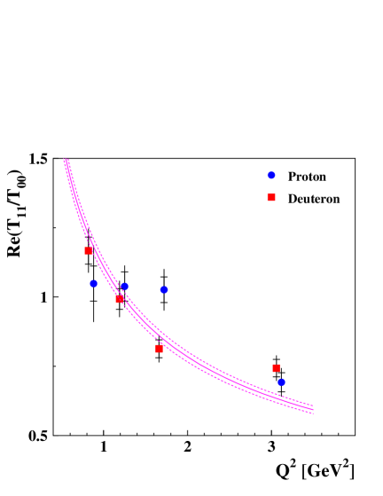
In the context of single-reggeon exchange, the isospin I=1𝐼1I=1 reggeon (ρ𝜌\rho, a2subscript𝑎2a_{2}, …) contribution to the amplitude of vector-meson production on the proton is of opposite sign to that on the neutron. In contrast, the I=0𝐼0I=0 reggeon (pomeron, ω𝜔\omega, f2subscript𝑓2f_{2}, …) contribution to the amplitude is of the same sign for both proton and neutron. Hence, the results on SDMEs and amplitude ratios should be different for proton and deuteron if I=1𝐼1I=1 and I=0𝐼0I=0 contributions to the amplitude interfere. By comparing proton and deuteron results, the fractional contribution of I=1𝐼1I=1 reggeons to the extracted amplitude ratios can be estimated.

4.2.4 Hierarchy of Amplitudes in the Kinematic Region of HERMES

In the HERMES kinematic region, the parameter β𝛽\beta is larger than 0.3 and the relative sizes of SDMEs measured in exclusive ρ0superscript𝜌0\rho^{0} production can be explained by the following hierarchy DC-24 :

|T00|2superscriptsubscript𝑇002\displaystyle|T_{00}|^{2} similar-to\displaystyle\sim |T11|2|U11|2>|T01|2|T10|2much-greater-thansuperscriptsubscript𝑇112superscriptsubscript𝑈112superscriptsubscript𝑇012much-greater-thansuperscriptsubscript𝑇102\displaystyle|T_{11}|^{2}\gg|U_{11}|^{2}>|T_{01}|^{2}\gg|T_{10}|^{2} (31)
similar-to\displaystyle\sim |T11|2>|U01|2|U10|2|U11|2,superscriptsubscript𝑇112superscriptsubscript𝑈012similar-tosuperscriptsubscript𝑈102similar-tosuperscriptsubscript𝑈112\displaystyle|T_{1-1}|^{2}>|U_{01}|^{2}\sim|U_{10}|^{2}\sim|U_{1-1}|^{2},

with the two largest amplitudes being T00subscript𝑇00T_{00} and T11subscript𝑇11T_{11}. The abbreviated notation UλVλγsubscript𝑈subscript𝜆𝑉subscript𝜆𝛾U_{\lambda_{V}\lambda_{\gamma}}, where

|UλVλγ|2|UλV12λγ12|2+|UλV12λγ12|2superscriptsubscript𝑈subscript𝜆𝑉subscript𝜆𝛾2superscriptsubscript𝑈subscript𝜆𝑉12subscript𝜆𝛾122superscriptsubscript𝑈subscript𝜆𝑉12subscript𝜆𝛾122\displaystyle|U_{\lambda_{V}\lambda_{\gamma}}|^{2}\equiv|U_{\lambda_{V}\frac{1}{2}\lambda_{\gamma}-\frac{1}{2}}|^{2}+|U_{\lambda_{V}\frac{1}{2}\lambda_{\gamma}\frac{1}{2}}|^{2} (32)

was introduced because, for UPE amplitudes, it is impossible to prove the dominance of those without nucleon helicity flip over those with helicity flip, in contrast to the NPE amplitudes. As shown in Eq. (31), the moduli of all the UPE amplitudes except U11subscript𝑈11U_{11} are smaller than those of the NPE amplitudes. The numerical estimate |U11|2/(|T11|2+ϵ|T00|2)0.11±0.04superscriptsubscript𝑈112superscriptsubscript𝑇112italic-ϵsuperscriptsubscript𝑇002plus-or-minus0.110.04|U_{11}|^{2}/(|T_{11}|^{2}+\epsilon|T_{00}|^{2})\approx 0.11\pm 0.04 obtained in Ref. DC-24 shows that the modulus of |U11|subscript𝑈11|U_{11}| is even larger than that of |T01|subscript𝑇01|T_{01}| (and the result of the fit done in the present work confirms this result) and the contribution of |U11|subscript𝑈11|U_{11}| to the SDMEs cannot be neglected. This contribution is suppressed by a factor γ4superscript𝛾4\gamma^{4} which is smaller than 0.010.010.01 in the HERMES kinematic region 3.03.03.0 GeV W6.5absent𝑊6.5\leq W\leq 6.5 GeV. If the UPE amplitude U11subscript𝑈11U_{11} is due to pion exchange, its contribution may be significant in the HERMES kinematic region because of the large pion-nucleon coupling constant gπNNsubscript𝑔𝜋𝑁𝑁g_{\pi NN}.

Contributions from small amplitudes can be appreciable if they are multiplied by the largest amplitudes T00subscript𝑇00T_{00} or T11subscript𝑇11T_{11} in the numerators of SDME formulas. As the small amplitudes T01subscript𝑇01T_{01}, T10subscript𝑇10T_{10}, and T11subscript𝑇11T_{1-1} are multiplied by the largest amplitudes (see Ref. SW and Appendix A of Ref. DC-24 ), five complex NPE amplitudes have to be considered in total, i.e. the four ratios T11/T00subscript𝑇11subscript𝑇00T_{11}/T_{00}, T01/T00subscript𝑇01subscript𝑇00T_{01}/T_{00}, T10/T00subscript𝑇10subscript𝑇00T_{10}/T_{00}, and T11/T00subscript𝑇11subscript𝑇00T_{1-1}/T_{00}. Concerning the ratio U11/T00subscript𝑈11subscript𝑇00U_{11}/T_{00}, only |U11|/|T00|subscript𝑈11subscript𝑇00|U_{11}|/|T_{00}| can be determined as there is no interference between UPE and NPE amplitudes for the case of an unpolarized target. The contribution of all other UPE amplitudes can be neglected DC-24 . In total, there are nine independent free parameters to be determined when fitting the angular distribution using the amplitude method.

4.3 Basic Formulas of the Amplitude Method

The exact formulas for SDMEs expressed in terms of helicity amplitudes are presented in Appendix A of Ref. DC-24 . In order to rewrite SDMEs in terms of the ratios of significant helicity amplitudes, we neglect the contributions from NPE nucleon helicity-flip amplitudes (using Eq. (16)) and from all UPE amplitudes except U11subscript𝑈11U_{11}. Then, dividing both the numerators and the denominator in the exact formulas for SDMEs by |T00|2superscriptsubscript𝑇002|T_{00}|^{2}, we arrive at approximate expressions for SDMEs in terms of certain amplitude ratios:

r0004superscriptsubscript𝑟0004\displaystyle r_{00}^{04} {ϵ+|t01|2}/N,similar-to-or-equalsabsentitalic-ϵsuperscriptsubscript𝑡012𝑁\displaystyle\simeq\{\epsilon+|t_{01}|^{2}\}/N\,, (33)
Re{r1004}Resuperscriptsubscript𝑟1004\displaystyle\mathrm{Re}\{r_{10}^{04}\} Re{ϵt10+12t01(t11t11)}/N,similar-to-or-equalsabsentReitalic-ϵsubscript𝑡1012subscript𝑡01superscriptsubscript𝑡11subscript𝑡11𝑁\displaystyle\simeq\mathrm{Re}\{\epsilon t_{10}+\frac{1}{2}t_{01}(t_{11}-t_{1-1})^{*}\}/N\,, (34)
r1104superscriptsubscript𝑟1104\displaystyle r_{1-1}^{04} Re{ϵ|t10|2+t11t11}/N,similar-to-or-equalsabsentReitalic-ϵsuperscriptsubscript𝑡102subscript𝑡11superscriptsubscript𝑡11𝑁\displaystyle\simeq\mathrm{Re}\{-\epsilon|t_{10}|^{2}+t_{1-1}t_{11}^{*}\}/N\,, (35)
r111superscriptsubscript𝑟111\displaystyle r_{11}^{1} Re{t11t11}/N,similar-to-or-equalsabsentResubscript𝑡11superscriptsubscript𝑡11𝑁\displaystyle\simeq\mathrm{Re}\{t_{1-1}t_{11}^{*}\}/N\,, (36)
r001superscriptsubscript𝑟001\displaystyle r_{00}^{1} |t01|2/N,similar-to-or-equalsabsentsuperscriptsubscript𝑡012𝑁\displaystyle\simeq-|t_{01}|^{2}/N\,, (37)
Re{r101}Resuperscriptsubscript𝑟101\displaystyle\mathrm{Re}\{r_{10}^{1}\} 12Re{t01(t11t11)}/N,similar-to-or-equalsabsent12Resubscript𝑡01superscriptsubscript𝑡11subscript𝑡11𝑁\displaystyle\simeq\frac{1}{2}\mathrm{Re}\{-t_{01}(t_{11}-t_{1-1})^{*}\}/N\,, (38)
r111superscriptsubscript𝑟111\displaystyle r_{1-1}^{1} 12{|t11|2+|t11|2|u11|2}/N,similar-to-or-equalsabsent12superscriptsubscript𝑡112superscriptsubscript𝑡112superscriptsubscript𝑢112𝑁\displaystyle\simeq\frac{1}{2}\{|t_{11}|^{2}+|t_{1-1}|^{2}-|u_{11}|^{2}\}/N\,, (39)
Im{r102}Imsuperscriptsubscript𝑟102\displaystyle\mathrm{Im}\{r_{10}^{2}\} 12Re{t01(t11+t11)}/N,similar-to-or-equalsabsent12Resubscript𝑡01superscriptsubscript𝑡11subscript𝑡11𝑁\displaystyle\simeq\frac{1}{2}\mathrm{Re}\{t_{01}(t_{11}+t_{1-1})^{*}\}/N\,, (40)
Im{r112}Imsuperscriptsubscript𝑟112\displaystyle\mathrm{Im}\{r_{1-1}^{2}\} 12{|t11|2+|t11|2+|u11|2}/N,similar-to-or-equalsabsent12superscriptsubscript𝑡112superscriptsubscript𝑡112superscriptsubscript𝑢112𝑁\displaystyle\simeq\frac{1}{2}\{-|t_{11}|^{2}+|t_{1-1}|^{2}+|u_{11}|^{2}\}/N\,, (41)
r115superscriptsubscript𝑟115\displaystyle r_{11}^{5} 12Re{t10(t11t11)}/N,similar-to-or-equalsabsent12Resubscript𝑡10superscriptsubscript𝑡11subscript𝑡11𝑁\displaystyle\simeq\frac{1}{\sqrt{2}}\mathrm{Re}\{t_{10}(t_{11}-t_{1-1})^{*}\}/N\,, (42)
r005superscriptsubscript𝑟005\displaystyle r_{00}^{5} 2Re{t01}/N,similar-to-or-equalsabsent2Resubscript𝑡01𝑁\displaystyle\simeq\sqrt{2}\mathrm{Re}\{t_{01}\}/N\,, (43)
Re{r105}Resuperscriptsubscript𝑟105\displaystyle\mathrm{Re}\{r_{10}^{5}\} 18Re{2t10t01+(t11t11)}/N,similar-to-or-equalsabsent18Re2subscript𝑡10superscriptsubscript𝑡01subscript𝑡11subscript𝑡11𝑁\displaystyle\simeq\frac{1}{\sqrt{8}}\mathrm{Re}\{2t_{10}t_{01}^{*}+(t_{11}-t_{1-1})\}/N\,, (44)
r115superscriptsubscript𝑟115\displaystyle r_{1-1}^{5} 12Re{t10(t11t11)}/N,similar-to-or-equalsabsent12Resubscript𝑡10superscriptsubscript𝑡11subscript𝑡11𝑁\displaystyle\simeq\frac{1}{\sqrt{2}}\mathrm{Re}\{-t_{10}(t_{11}-t_{1-1})^{*}\}/N\,, (45)
Im{r106}Imsuperscriptsubscript𝑟106\displaystyle\mathrm{Im}\{r_{10}^{6}\} 18Re{t11+t11}/N,similar-to-or-equalsabsent18Resubscript𝑡11subscript𝑡11𝑁\displaystyle\simeq-\frac{1}{\sqrt{8}}\mathrm{Re}\{t_{11}+t_{1-1}\}/N\,, (46)
Im{r116}Imsubscriptsuperscript𝑟611\displaystyle\mathrm{Im}\{r^{6}_{1-1}\} 12Re{t10(t11+t11)}/N,similar-to-or-equalsabsent12Resubscript𝑡10superscriptsubscript𝑡11subscript𝑡11𝑁\displaystyle\simeq\frac{1}{\sqrt{2}}\mathrm{Re}\{t_{10}(t_{11}+t_{1-1})^{*}\}/N\,, (47)
Im{r103}Imsuperscriptsubscript𝑟103\displaystyle\mathrm{Im}\{r_{10}^{3}\} 12Im{t01(t11+t11)}/N,similar-to-or-equalsabsent12Imsubscript𝑡01superscriptsubscript𝑡11subscript𝑡11𝑁\displaystyle\simeq-\frac{1}{2}\mathrm{Im}\{t_{01}(t_{11}+t_{1-1})^{*}\}/N\,, (48)
Im{r113}Imsuperscriptsubscript𝑟113\displaystyle\mathrm{Im}\{r_{1-1}^{3}\} Im{t11t11}/N,similar-to-or-equalsabsentImsubscript𝑡11superscriptsubscript𝑡11𝑁\displaystyle\simeq-\mathrm{Im}\{t_{1-1}t_{11}^{*}\}/N\;, (49)
Im{r107}Imsuperscriptsubscript𝑟107\displaystyle\mathrm{Im}\{r_{10}^{7}\} 18Im{t11+t11}/N,similar-to-or-equalsabsent18Imsubscript𝑡11subscript𝑡11𝑁\displaystyle\simeq\frac{1}{\sqrt{8}}\mathrm{Im}\{t_{11}+t_{1-1}\}/N\,, (50)
Im{r117}Imsuperscriptsubscript𝑟117\displaystyle\mathrm{Im}\{r_{1-1}^{7}\} 12Im{t10(t11+t11)}/N,similar-to-or-equalsabsent12Imsubscript𝑡10superscriptsubscript𝑡11subscript𝑡11𝑁\displaystyle\simeq\frac{1}{\sqrt{2}}\mathrm{Im}\{t_{10}(t_{11}+t_{1-1})^{*}\}/N, (51)
r118subscriptsuperscript𝑟811\displaystyle r^{8}_{11} 12Im{t10(t11t11)}/N,similar-to-or-equalsabsent12Imsubscript𝑡10superscriptsubscript𝑡11subscript𝑡11𝑁\displaystyle\simeq-\frac{1}{\sqrt{2}}\mathrm{Im}\{t_{10}(t_{11}-t_{1-1})^{*}\}/N\,, (52)
r008superscriptsubscript𝑟008\displaystyle r_{00}^{8} 2Im{t01}/N,similar-to-or-equalsabsent2Imsubscript𝑡01𝑁\displaystyle\simeq\sqrt{2}\mathrm{Im}\{t_{01}\}/N\,, (53)
Re{r108}Resuperscriptsubscript𝑟108\displaystyle\mathrm{Re}\{r_{10}^{8}\} 18Im{2t10t01+t11t11}/N,similar-to-or-equalsabsent18Im2subscript𝑡10superscriptsubscript𝑡01subscript𝑡11subscript𝑡11𝑁\displaystyle\simeq\frac{1}{\sqrt{8}}\mathrm{Im}\{-2t_{10}t_{01}^{*}+t_{11}-t_{1-1}\}/N\,, (54)
r118superscriptsubscript𝑟118\displaystyle r_{1-1}^{8} 12Im{t10(t11t11)}/Nsimilar-to-or-equalsabsent12Imsubscript𝑡10superscriptsubscript𝑡11subscript𝑡11𝑁\displaystyle\simeq\frac{1}{\sqrt{2}}\mathrm{Im}\{t_{10}(t_{11}-t_{1-1})^{*}\}/N (55)

where the normalization factor N=𝒩/|T00|2𝑁𝒩superscriptsubscript𝑇002N=\mathcal{N}/|T_{00}|^{2} is defined in accordance with Eqs. (19)-(21) by

N𝑁\displaystyle N =\displaystyle= NT+ϵNL,subscript𝑁𝑇italic-ϵsubscript𝑁𝐿\displaystyle N_{T}+\epsilon N_{L},
NTsubscript𝑁𝑇\displaystyle N_{T} similar-to-or-equals\displaystyle\simeq |t11|2+|t01|2+|t11|2+|u11|2,superscriptsubscript𝑡112superscriptsubscript𝑡012superscriptsubscript𝑡112superscriptsubscript𝑢112\displaystyle|t_{11}|^{2}+|t_{01}|^{2}+|t_{1-1}|^{2}+|u_{11}|^{2},
NLsubscript𝑁𝐿\displaystyle N_{L} similar-to-or-equals\displaystyle\simeq 1+2|t10|2.12superscriptsubscript𝑡102\displaystyle 1+2|t_{10}|^{2}. (56)

Here tλVλγTλVλγ/T00subscript𝑡subscript𝜆𝑉subscript𝜆𝛾subscript𝑇subscript𝜆𝑉subscript𝜆𝛾subscript𝑇00t_{\lambda_{V}\lambda_{\gamma}}\equiv T_{\lambda_{V}\lambda_{\gamma}}/T_{00} and |u11|2|U11|2/|T00|2superscriptsubscript𝑢112superscriptsubscript𝑈112superscriptsubscript𝑇002|u_{11}|^{2}\equiv|U_{11}|^{2}/|T_{00}|^{2} with |U11|2superscriptsubscript𝑈112|U_{11}|^{2} defined in Eq. (32). There are nine independent real functions in Eqs. (33-56), namely: Re(t11)Resubscript𝑡11\mathrm{Re}(t_{11}), Im(t11)Imsubscript𝑡11\mathrm{Im}(t_{11}), Re(t01)Resubscript𝑡01\mathrm{Re}(t_{01}), Im(t01)Imsubscript𝑡01\mathrm{Im}(t_{01}), Re(t10)Resubscript𝑡10\mathrm{Re}(t_{10}), Im(t10)Imsubscript𝑡10\mathrm{Im}(t_{10}), Re(t11)Resubscript𝑡11\mathrm{Re}(t_{1-1}), Im(t11)Imsubscript𝑡11\mathrm{Im}(t_{1-1}), and |u11|subscript𝑢11|u_{11}|. Equations (33-56) are the basis for the extraction of the helicity amplitude ratios from the measured angular distributions and also for the calculation of SDMEs from amplitude ratios (see Sec. 6.5).

5 The HERMES Experiment

A detailed description of the HERMES experiment at DESY can be found in Ref. herspec . The data analyzed in this paper were collected between the years 1996 and 2005. A longitudinally polarized positron or electron beam of 27.627.627.6 GeV was scattered from pure hydrogen or deuterium gas targets internal to the HERA lepton storage ring. The lepton beam was transversely polarized due to an asymmetry in the emission of synchrotron-radiation ST in the field of the dipole magnets. The transverse beam polarization was transformed locally into longitudinal polarization at the interaction point by spin rotators located upstream and downstream of the HERMES apparatus. The helicity of the beam was typically reversed every two months. For both positive and negative beam helicities, the beam polarization was continuously measured by two Compton polarimeters BAR ; BECK . The average beam polarization for the hydrogen (deuterium) data set was 0.45 (0.47) after requiring 0.15<PB<0.80.15subscript𝑃𝐵0.80.15<P_{B}<0.8 in the analysis process, and the fractional uncertainty of the beam polarization was 3.4% (2.0%) BAR ; BECK . Some of the data were collected with longitudinally or transversely polarized targets. However, the time-averaged polarization of the polarized targets was negligible, while the rapid (60-180s) reversal of the polarization direction minimized polarization bias due to detector effects.

HERMES was a forward spectrometer herspec in which both scattered lepton and produced hadrons were detected within an angular acceptance of ±plus-or-minus\pm170 mrad horizontally, and ±(40140)plus-or-minus40140\pm(40-140) mrad vertically. The tracking system had a momentum resolution of about 1.5%percent1.51.5\% and an angular resolution of about 111 mrad. Lepton identification was accomplished using a transition-radiation detector, a preshower scintillator counter, and the electromagnetic calorimeter. The particle identification system included a gas threshold C˘˘C\breve{\mathrm{C}}erenkov counter, which was replaced in 1998 by a dual-radiator ring-imaging C˘˘C\breve{\mathrm{C}}erenkov detector RICH . Combining the responses of these detectors in a likelihood method led to an average lepton identification efficiency of 98% with a hadron contamination of less than 1%. The event sample used in this analysis is exactly the same as that used in Ref. DC-24 .

6 Extraction of Amplitude Ratios

The measurement of the angular distribution of the scattered electrons/positrons and the pions from the decay ρ0π+πsuperscript𝜌0superscript𝜋superscript𝜋\rho^{0}\to\pi^{+}\pi^{-} is the basis for the extraction of spin density matrix elements rλVμVηsubscriptsuperscript𝑟𝜂subscript𝜆𝑉subscript𝜇𝑉r^{\eta}_{\lambda_{V}\mu_{V}} in the SDME method and of helicity amplitude ratios tλVλγsubscript𝑡subscript𝜆𝑉subscript𝜆𝛾t_{\lambda_{V}\lambda_{\gamma}} and |u11|subscript𝑢11|u_{11}| in the amplitude method. For a polarized lepton beam and an unpolarized target, the angular distribution of the pions is given by relations (24-26) in Sec. 3.3 (see also Refs. SW ; DC-24 ), where the SDMEs are expressed in terms of helicity amplitude ratios according to Eqs. (33-56).

6.1 Binned Maximum Likelihood Method

Amplitude ratios are extracted with the same binned maximum likelihood method as in the previous SDME analysis (see Sec. 6 of Ref. DC-24 ). In brief, the amplitude ratios in each of the kinematic bins are obtained by minimizing the difference between the 3-dimensional (cosθ,ϕ,Φ)𝜃italic-ϕΦ(\cos\theta,\phi,\Phi) angular distribution of the experimental events and that of a sample of fully reconstructed Monte Carlo events. The latter are generated isotropically in (cosθ,ϕ,Φ)𝜃italic-ϕΦ(\cos\theta,\phi,\Phi) using the rhoMC generator tytgat ; ami-phd for exclusive ρ0superscript𝜌0\rho^{0} simulated in the instrumental context of the spectrometer, and passed through the same reconstruction chain as the experimental data. The generated Monte Carlo events are iteratively reweighted with the angular distribution given by Eqs. (24-26), with the amplitude ratios treated as free parameters.

The minimization itself and the uncertainty calculation are performed using the MINUIT package CERN-CN . More details can be found in Ref. DC-24 .

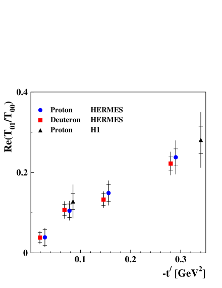
6.2 Results on Amplitude Ratios in Bins of Q2superscript𝑄2Q^{2} and tsuperscript𝑡-t^{\prime}

bin Q2delimited-⟨⟩superscript𝑄2\langle Q^{2}\rangle, GeV2 tdelimited-⟨⟩superscript𝑡\langle-t^{\prime}\rangle, GeV2 bin Q2delimited-⟨⟩superscript𝑄2\langle Q^{2}\rangle, GeV2 tdelimited-⟨⟩superscript𝑡\langle-t^{\prime}\rangle, GeV2
q1subscript𝑞1q_{1}t1subscript𝑡1t_{1} 0.817 0.019 q3subscript𝑞3q_{3}t1subscript𝑡1t_{1} 1.658 0.019
q1subscript𝑞1q_{1}t2subscript𝑡2t_{2} 0.823 0.068 q3subscript𝑞3q_{3}t2subscript𝑡2t_{2} 1.660 0.068
q1subscript𝑞1q_{1}t3subscript𝑡3t_{3} 0.821 0.146 q3subscript𝑞3q_{3}t3subscript𝑡3t_{3} 1.663 0.146
q1subscript𝑞1q_{1}t4subscript𝑡4t_{4} 0.815 0.280 q3subscript𝑞3q_{3}t4subscript𝑡4t_{4} 1.663 0.282
q2subscript𝑞2q_{2}t1subscript𝑡1t_{1} 1.184 0.019 q4subscript𝑞4q_{4}t1subscript𝑡1t_{1} 2.996 0.019
q2subscript𝑞2q_{2}t2subscript𝑡2t_{2} 1.188 0.068 q4subscript𝑞4q_{4}t2subscript𝑡2t_{2} 3.056 0.068
q2subscript𝑞2q_{2}t3subscript𝑡3t_{3} 1.189 0.145 q4subscript𝑞4q_{4}t3subscript𝑡3t_{3} 3.076 0.146
q2subscript𝑞2q_{2}t4subscript𝑡4t_{4} 1.188 0.282 q4subscript𝑞4q_{4}t4subscript𝑡4t_{4} 3.134 0.284
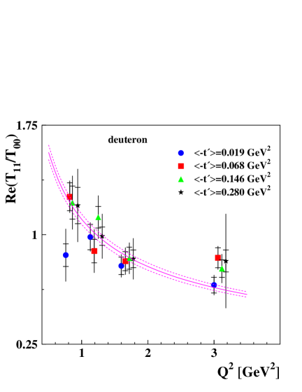
Table 1: Mean values of kinematic variables for 16 bins. The limits of the q1subscript𝑞1q_{1}, q2subscript𝑞2q_{2}, q3subscript𝑞3q_{3}, and q4subscript𝑞4q_{4} bins for Q2superscript𝑄2Q^{2} are 0.5; 1.0; 1.4; 2.0; 7.0 GeV2 while those of the t1subscript𝑡1t_{1}, t2subscript𝑡2t_{2}, t3subscript𝑡3t_{3}, and t4subscript𝑡4t_{4} bins for tsuperscript𝑡-t^{\prime} are the following: 0.0; 0.04; 0.10; 0.20; 0.40 GeV2.

Ratios of helicity amplitudes are extracted in a two-dimensional (Q2superscript𝑄2Q^{2}, tsuperscript𝑡-t^{\prime}) binning from the same HERMES proton and deuteron data sets as were used for the SDME analysis of Ref. DC-24 . The four Q2superscript𝑄2Q^{2} bins are denoted as q1subscript𝑞1q_{1}, q2subscript𝑞2q_{2}, q3subscript𝑞3q_{3}, and q4subscript𝑞4q_{4} defined by the limits 0.50.50.5, 1.01.01.0, 1.41.41.4, 2.02.02.0, 7.07.07.0 GeV2. The four tsuperscript𝑡-t^{\prime} bins are denoted as t1subscript𝑡1t_{1}, t2subscript𝑡2t_{2}, t3subscript𝑡3t_{3}, and t4subscript𝑡4t_{4} defined by the limits 0.00.00.0, 0.040.040.04, 0.100.100.10, 0.200.200.20, 0.400.400.40 GeV2. The mean values of Q2superscript𝑄2Q^{2} and tsuperscript𝑡-t^{\prime} in each bin are presented in Tab. 1. The results of the extraction of the amplitude ratios in 16 bins are presented in Tab. 2 for the proton data and in Tab. 3 for the deuteron data. In every (Q2superscript𝑄2Q^{2}, tsuperscript𝑡-t^{\prime}) bin, the nine free parameters are obtained from a fit to the 3-dimensional angular distribution without subtracting the background from semi-inclusive deep-inelastic scattering (SIDIS). The SIDIS background under the exclusive peak, i.e., in the region 11-1 GeV <ΔE<0.6absentΔ𝐸0.6<\Delta E<0.6 GeV, is estimated using the PYTHIA Monte Carlo generator pyth (see Ref. DC-24 for more details) and its effect is assigned as a systematic uncertainty.

Ratio q1subscript𝑞1q_{1}t1subscript𝑡1t_{1} q1subscript𝑞1q_{1}t2subscript𝑡2t_{2} q1subscript𝑞1q_{1}t3subscript𝑡3t_{3} q1subscript𝑞1q_{1}t4subscript𝑡4t_{4}
Re(t11)Resubscript𝑡11\mathrm{Re}(t_{11}) 0.975±0.121±0.297plus-or-minus0.9750.1210.2970.975\pm 0.121\pm 0.297 0.961±0.101±0.213plus-or-minus0.9610.1010.2130.961\pm 0.101\pm 0.213 1.363±0.140±0.309plus-or-minus1.3630.1400.3091.363\pm 0.140\pm 0.309 1.037±0.176±0.230plus-or-minus1.0370.1760.2301.037\pm 0.176\pm 0.230
Im(t11)Imsubscript𝑡11\mathrm{Im}(t_{11}) 0.542±0.187±0.052plus-or-minus0.5420.1870.0520.542\pm 0.187\pm 0.052 0.285±0.145±0.174plus-or-minus0.2850.1450.1740.285\pm 0.145\pm 0.174 0.082±0.285±0.104plus-or-minus0.0820.2850.1040.082\pm 0.285\pm 0.104 0.783±0.147±0.213plus-or-minus0.7830.1470.2130.783\pm 0.147\pm 0.213
Re(t01)Resubscript𝑡01\mathrm{Re}(t_{01}) 0.025±0.044±0.056plus-or-minus0.0250.0440.0560.025\pm 0.044\pm 0.056 0.112±0.036±0.047plus-or-minus0.1120.0360.0470.112\pm 0.036\pm 0.047 0.214±0.064±0.050plus-or-minus0.2140.0640.0500.214\pm 0.064\pm 0.050 0.182±0.048±0.116plus-or-minus0.1820.0480.1160.182\pm 0.048\pm 0.116
Im(t01)Imsubscript𝑡01\mathrm{Im}(t_{01}) 0.098±0170±0.211plus-or-minus0.09801700.211-0.098\pm 0170\pm 0.211 0.111±0.111±0.136plus-or-minus0.1110.1110.1360.111\pm 0.111\pm 0.136 0.315±0.120±0.073plus-or-minus0.3150.1200.0730.315\pm 0.120\pm 0.073 0.107±0.108±0.107plus-or-minus0.1070.1080.1070.107\pm 0.108\pm 0.107
Re(t10)Resubscript𝑡10\mathrm{Re}(t_{10}) 0.037±0.038±0.050plus-or-minus0.0370.0380.0500.037\pm 0.038\pm 0.050 0.049±0.039±0.024plus-or-minus0.0490.0390.024-0.049\pm 0.039\pm 0.024 0.024±0.039±0.026plus-or-minus0.0240.0390.0260.024\pm 0.039\pm 0.026 0.010±0.056±0.043plus-or-minus0.0100.0560.043-0.010\pm 0.056\pm 0.043
Im(t10)Imsubscript𝑡10\mathrm{Im}(t_{10}) 0.067±0.064±0.156plus-or-minus0.0670.0640.156-0.067\pm 0.064\pm 0.156 0.066±0.068±0.009plus-or-minus0.0660.0680.009-0.066\pm 0.068\pm 0.009 0.005±0.069±0.023plus-or-minus0.0050.0690.0230.005\pm 0.069\pm 0.023 0.050±0.067±0.021plus-or-minus0.0500.0670.0210.050\pm 0.067\pm 0.021
Re(t11)Resubscript𝑡11\mathrm{Re}(t_{1-1}) 0.110±0.042±0.045plus-or-minus0.1100.0420.045-0.110\pm 0.042\pm 0.045 0.021±0.037±0.079plus-or-minus0.0210.0370.079-0.021\pm 0.037\pm 0.079 0.037±0.043±0.043plus-or-minus0.0370.0430.043-0.037\pm 0.043\pm 0.043 0.020±0.056±0.040plus-or-minus0.0200.0560.0400.020\pm 0.056\pm 0.040
Im(t11)Imsubscript𝑡11\mathrm{Im}(t_{1-1}) 0.178±0.087±0.349plus-or-minus0.1780.0870.3490.178\pm 0.087\pm 0.349 0.147±0.092±0.055plus-or-minus0.1470.0920.055-0.147\pm 0.092\pm 0.055 0.124±0.100±0.079plus-or-minus0.1240.1000.079-0.124\pm 0.100\pm 0.079 0.172±0.079±0.104plus-or-minus0.1720.0790.104-0.172\pm 0.079\pm 0.104
|u11|subscript𝑢11|u_{11}| 0.329±0.070±0.021plus-or-minus0.3290.0700.0210.329\pm 0.070\pm 0.021 0.424±0.049±0.032plus-or-minus0.4240.0490.0320.424\pm 0.049\pm 0.032 0.391±0.063±0.124plus-or-minus0.3910.0630.1240.391\pm 0.063\pm 0.124 0.357±0.077±0.070plus-or-minus0.3570.0770.0700.357\pm 0.077\pm 0.070
Ratio q2subscript𝑞2q_{2}t1subscript𝑡1t_{1} q2subscript𝑞2q_{2}t2subscript𝑡2t_{2} q2subscript𝑞2q_{2}t3subscript𝑡3t_{3} q2subscript𝑞2q_{2}t4subscript𝑡4t_{4}
Re(t11)Resubscript𝑡11\mathrm{Re}(t_{11}) 1.138±0.143±0.021plus-or-minus1.1380.1430.0211.138\pm 0.143\pm 0.021 0.996±0.106±0.084plus-or-minus0.9960.1060.0840.996\pm 0.106\pm 0.084 1.079±0.094±0.135plus-or-minus1.0790.0940.1351.079\pm 0.094\pm 0.135 0.925±0.097±0.139plus-or-minus0.9250.0970.1390.925\pm 0.097\pm 0.139
Im(t11)Imsubscript𝑡11\mathrm{Im}(t_{11}) 0.282±0.268±0.212plus-or-minus0.2820.2680.2120.282\pm 0.268\pm 0.212 0.386±0.125±0.039plus-or-minus0.3860.1250.0390.386\pm 0.125\pm 0.039 0.342±0.162±0.159plus-or-minus0.3420.1620.1590.342\pm 0.162\pm 0.159 0.289±0.156±0.141plus-or-minus0.2890.1560.1410.289\pm 0.156\pm 0.141
Re(t01)Resubscript𝑡01\mathrm{Re}(t_{01}) 0.044±0.051±0.009plus-or-minus0.0440.0510.0090.044\pm 0.051\pm 0.009 0.116±0.037±0.061plus-or-minus0.1160.0370.0610.116\pm 0.037\pm 0.061 0.113±0.035±0.030plus-or-minus0.1130.0350.0300.113\pm 0.035\pm 0.030 0.250±0.043±0.075plus-or-minus0.2500.0430.0750.250\pm 0.043\pm 0.075
Im(t01)Imsubscript𝑡01\mathrm{Im}(t_{01}) 0.073±0.146±0.137plus-or-minus0.0730.1460.1370.073\pm 0.146\pm 0.137 0.327±0.099±0.083plus-or-minus0.3270.0990.0830.327\pm 0.099\pm 0.083 0.009±0.141±0.069plus-or-minus0.0090.1410.069-0.009\pm 0.141\pm 0.069 0.265±0.107±0.055plus-or-minus0.2650.1070.0550.265\pm 0.107\pm 0.055
Re(t10)Resubscript𝑡10\mathrm{Re}(t_{10}) 0.001±0.054±0.011plus-or-minus0.0010.0540.0110.001\pm 0.054\pm 0.011 0.054±0.034±0.033plus-or-minus0.0540.0340.033-0.054\pm 0.034\pm 0.033 0.032±0.030±0.015plus-or-minus0.0320.0300.0150.032\pm 0.030\pm 0.015 0.065±0.032±0.020plus-or-minus0.0650.0320.020-0.065\pm 0.032\pm 0.020
Im(t10)Imsubscript𝑡10\mathrm{Im}(t_{10}) 0.081±0.073±0.154plus-or-minus0.0810.0730.154-0.081\pm 0.073\pm 0.154 0.064±0.073±0.058plus-or-minus0.0640.0730.0580.064\pm 0.073\pm 0.058 0.006±0.070±0.027plus-or-minus0.0060.0700.0270.006\pm 0.070\pm 0.027 0.063±0.073±0.057plus-or-minus0.0630.0730.0570.063\pm 0.073\pm 0.057
Re(t11)Resubscript𝑡11\mathrm{Re}(t_{1-1}) 0.001±0.045±0.015plus-or-minus0.0010.0450.0150.001\pm 0.045\pm 0.015 0.023±0.040±0.018plus-or-minus0.0230.0400.0180.023\pm 0.040\pm 0.018 0.017±0.036±0.021plus-or-minus0.0170.0360.021-0.017\pm 0.036\pm 0.021 0.073±0.035±0.019plus-or-minus0.0730.0350.019-0.073\pm 0.035\pm 0.019
Im(t11)Imsubscript𝑡11\mathrm{Im}(t_{1-1}) 0.041±0.137±0.271plus-or-minus0.0410.1370.271-0.041\pm 0.137\pm 0.271 0.002±0.078±0.019plus-or-minus0.0020.0780.0190.002\pm 0.078\pm 0.019 0.084±0.107±0.024plus-or-minus0.0840.1070.024-0.084\pm 0.107\pm 0.024 0.099±0.069±0.034plus-or-minus0.0990.0690.034-0.099\pm 0.069\pm 0.034
|u11|subscript𝑢11|u_{11}| 0.499±0.040±0.039plus-or-minus0.4990.0400.0390.499\pm 0.040\pm 0.039 0.429±0.042±0.081plus-or-minus0.4290.0420.0810.429\pm 0.042\pm 0.081 0.418±0.046±0.119plus-or-minus0.4180.0460.1190.418\pm 0.046\pm 0.119 0.359±0.055±0.055plus-or-minus0.3590.0550.0550.359\pm 0.055\pm 0.055
Ratio q3subscript𝑞3q_{3}t1subscript𝑡1t_{1} q3subscript𝑞3q_{3}t2subscript𝑡2t_{2} q3subscript𝑞3q_{3}t3subscript𝑡3t_{3} q3subscript𝑞3q_{3}t4subscript𝑡4t_{4}
Re(t11)Resubscript𝑡11\mathrm{Re}(t_{11}) 1.029±0.104±0.039plus-or-minus1.0290.1040.0391.029\pm 0.104\pm 0.039 1.088±0.098±0.083plus-or-minus1.0880.0980.0831.088\pm 0.098\pm 0.083 0.878±0.079±0.202plus-or-minus0.8780.0790.2020.878\pm 0.079\pm 0.202 0.975±0.096±0.228plus-or-minus0.9750.0960.2280.975\pm 0.096\pm 0.228
Im(t11)Imsubscript𝑡11\mathrm{Im}(t_{11}) 0.257±0.131±0.151plus-or-minus0.2570.1310.1510.257\pm 0.131\pm 0.151 0.479±0.111±0.050plus-or-minus0.4790.1110.0500.479\pm 0.111\pm 0.050 0.513±0.102±0.385plus-or-minus0.5130.1020.3850.513\pm 0.102\pm 0.385 0.280±0.176±0.365plus-or-minus0.2800.1760.3650.280\pm 0.176\pm 0.365
Re(t01)Resubscript𝑡01\mathrm{Re}(t_{01}) 0.052±0.039±0.052plus-or-minus0.0520.0390.052-0.052\pm 0.039\pm 0.052 0.008±0.032±0.060plus-or-minus0.0080.0320.0600.008\pm 0.032\pm 0.060 0.113±0.035±0.081plus-or-minus0.1130.0350.0810.113\pm 0.035\pm 0.081 0.194±0.044±0.064plus-or-minus0.1940.0440.0640.194\pm 0.044\pm 0.064
Im(t01)Imsubscript𝑡01\mathrm{Im}(t_{01}) 0.357±0.127±0.480plus-or-minus0.3570.1270.4800.357\pm 0.127\pm 0.480 0.100±0.100±0.004plus-or-minus0.1000.1000.0040.100\pm 0.100\pm 0.004 0.123±0.092±0.275plus-or-minus0.1230.0920.2750.123\pm 0.092\pm 0.275 0.100±0.108±0.406plus-or-minus0.1000.1080.406-0.100\pm 0.108\pm 0.406
Re(t100\mathrm{Re}(t_{10}0 0.074±0.028±0.021plus-or-minus0.0740.0280.0210.074\pm 0.028\pm 0.021 0.043±0.028±0.011plus-or-minus0.0430.0280.0110.043\pm 0.028\pm 0.011 0.007±0.034±0.032plus-or-minus0.0070.0340.032-0.007\pm 0.034\pm 0.032 0.032±0.038±0.036plus-or-minus0.0320.0380.036-0.032\pm 0.038\pm 0.036
Im(t10)Imsubscript𝑡10\mathrm{Im}(t_{10}) 0.051±0.067±0.042plus-or-minus0.0510.0670.042-0.051\pm 0.067\pm 0.042 0.129±0.058±0.031plus-or-minus0.1290.0580.031-0.129\pm 0.058\pm 0.031 0.075±0.053±0.173plus-or-minus0.0750.0530.1730.075\pm 0.053\pm 0.173 0.025±0.113±0.120plus-or-minus0.0250.1130.1200.025\pm 0.113\pm 0.120
Re(t11)Resubscript𝑡11\mathrm{Re}(t_{1-1}) 0.013±0.038±0.021plus-or-minus0.0130.0380.021-0.013\pm 0.038\pm 0.021 0.019±0.035±0.037plus-or-minus0.0190.0350.037-0.019\pm 0.035\pm 0.037 0.034±0.037±0.101plus-or-minus0.0340.0370.1010.034\pm 0.037\pm 0.101 0.044±0.036±0.065plus-or-minus0.0440.0360.065-0.044\pm 0.036\pm 0.065
Im(t11)Imsubscript𝑡11\mathrm{Im}(t_{1-1}) 0.108±0.090±0.236plus-or-minus0.1080.0900.2360.108\pm 0.090\pm 0.236 0.100±0.071±0.031plus-or-minus0.1000.0710.0310.100\pm 0.071\pm 0.031 0.186±0.071±0.071plus-or-minus0.1860.0710.071-0.186\pm 0.071\pm 0.071 0.037±0.098±0.185plus-or-minus0.0370.0980.1850.037\pm 0.098\pm 0.185
|u11|subscript𝑢11|u_{11}| 0.423±0.055±0.048plus-or-minus0.4230.0550.0480.423\pm 0.055\pm 0.048 0.323±0.068±0.084plus-or-minus0.3230.0680.0840.323\pm 0.068\pm 0.084 0.346±0.056±0.085plus-or-minus0.3460.0560.0850.346\pm 0.056\pm 0.085 0.445±0.050±0.191plus-or-minus0.4450.0500.1910.445\pm 0.050\pm 0.191
Ratio q4subscript𝑞4q_{4}t1subscript𝑡1t_{1} q4subscript𝑞4q_{4}t2subscript𝑡2t_{2} q4subscript𝑞4q_{4}t3subscript𝑡3t_{3} q4subscript𝑞4q_{4}t4subscript𝑡4t_{4}
Re(t11)Resubscript𝑡11\mathrm{Re}(t_{11}) 0.723±0.071±0.053plus-or-minus0.7230.0710.0530.723\pm 0.071\pm 0.053 0.706±0.068±0.039plus-or-minus0.7060.0680.0390.706\pm 0.068\pm 0.039 0.582±0.074±0.156plus-or-minus0.5820.0740.1560.582\pm 0.074\pm 0.156 0.650±0.063±0.117plus-or-minus0.6500.0630.1170.650\pm 0.063\pm 0.117
Im(t11)Imsubscript𝑡11\mathrm{Im}(t_{11}) 0.570±0.071±0.025plus-or-minus0.5700.0710.0250.570\pm 0.071\pm 0.025 0.657±0.061±0.066plus-or-minus0.6570.0610.0660.657\pm 0.061\pm 0.066 0.583±0.110±0.120plus-or-minus0.5830.1100.1200.583\pm 0.110\pm 0.120 0.488±0.067±0.119plus-or-minus0.4880.0670.1190.488\pm 0.067\pm 0.119
Re(t01)Resubscript𝑡01\mathrm{Re}(t_{01}) 0.062±0.031±0.007plus-or-minus0.0620.0310.0070.062\pm 0.031\pm 0.007 0.121±0.031±0.006plus-or-minus0.1210.0310.0060.121\pm 0.031\pm 0.006 0.190±0.054±0.021plus-or-minus0.1900.0540.0210.190\pm 0.054\pm 0.021 0.282±0.036±0.060plus-or-minus0.2820.0360.0600.282\pm 0.036\pm 0.060
Im(t01)Imsubscript𝑡01\mathrm{Im}(t_{01}) 0.011±0.069±0.019plus-or-minus0.0110.0690.0190.011\pm 0.069\pm 0.019 0.084±0.079±0.019plus-or-minus0.0840.0790.0190.084\pm 0.079\pm 0.019 0.129±0.0.57±0.154plus-or-minus0.1290.0.570.154-0.129\pm 0.0.57\pm 0.154 0.099±0.081±0.044plus-or-minus0.0990.0810.044-0.099\pm 0.081\pm 0.044
Re(t10)Resubscript𝑡10\mathrm{Re}(t_{10}) 0.013±0.030±0.011plus-or-minus0.0130.0300.011-0.013\pm 0.030\pm 0.011 0.046±0.035±0.008plus-or-minus0.0460.0350.008-0.046\pm 0.035\pm 0.008 0.095±0.025±0.118plus-or-minus0.0950.0250.1180.095\pm 0.025\pm 0.118 0.007±0.031±0.012plus-or-minus0.0070.0310.0120.007\pm 0.031\pm 0.012
Im(t10)Imsubscript𝑡10\mathrm{Im}(t_{10}) 0.010±0.052±0.010plus-or-minus0.0100.0520.0100.010\pm 0.052\pm 0.010 0.050±0.045±0.015plus-or-minus0.0500.0450.0150.050\pm 0.045\pm 0.015 0.181±0.060±0.258plus-or-minus0.1810.0600.258-0.181\pm 0.060\pm 0.258 0.003±0.044±0.058plus-or-minus0.0030.0440.0580.003\pm 0.044\pm 0.058
Re(t11)Resubscript𝑡11\mathrm{Re}(t_{1-1}) 0.000±0.034±0.007plus-or-minus0.0000.0340.0070.000\pm 0.034\pm 0.007 0.065±0.034±0.007plus-or-minus0.0650.0340.0070.065\pm 0.034\pm 0.007 0.027±0.040±0.033plus-or-minus0.0270.0400.0330.027\pm 0.040\pm 0.033 0.024±0.031±0.011plus-or-minus0.0240.0310.0110.024\pm 0.031\pm 0.011
Im(t11)Imsubscript𝑡11\mathrm{Im}(t_{1-1}) 0.029±0.056±0.005plus-or-minus0.0290.0560.0050.029\pm 0.056\pm 0.005 0.068±0.048±0.015plus-or-minus0.0680.0480.015-0.068\pm 0.048\pm 0.015 0.038±0.040±0.142plus-or-minus0.0380.0400.142-0.038\pm 0.040\pm 0.142 0.036±0.051±0.066plus-or-minus0.0360.0510.066-0.036\pm 0.051\pm 0.066
|u11|subscript𝑢11|u_{11}| 0.451±0.049±0.024plus-or-minus0.4510.0490.0240.451\pm 0.049\pm 0.024 0.306±0.061±0.032plus-or-minus0.3060.0610.0320.306\pm 0.061\pm 0.032 0.383±0.067±0.097plus-or-minus0.3830.0670.0970.383\pm 0.067\pm 0.097 0.380±0.044±0.091plus-or-minus0.3800.0440.0910.380\pm 0.044\pm 0.091
Table 2: Ratios of helicity amplitudes in Q2superscript𝑄2Q^{2} and tsuperscript𝑡-t^{\prime} bins for proton data. The mean values of Q2superscript𝑄2Q^{2} and tsuperscript𝑡-t^{\prime} for all 16 bins are given in Tab. 1. The notations tkjsubscript𝑡𝑘𝑗t_{kj} and |u11|subscript𝑢11|u_{11}| are used for the amplitude ratios Tkj/T00subscript𝑇𝑘𝑗subscript𝑇00T_{kj}/T_{00} and |U11/T00|subscript𝑈11subscript𝑇00|U_{11}/T_{00}|, respectively. The first uncertainties are statistical, the second are systematic.
Ratio q1subscript𝑞1q_{1}t1subscript𝑡1t_{1} q1subscript𝑞1q_{1}t2subscript𝑡2t_{2} q1subscript𝑞1q_{1}t3subscript𝑡3t_{3} q1subscript𝑞1q_{1}t4subscript𝑡4t_{4}
Re(t11)Resubscript𝑡11\mathrm{Re}(t_{11}) 0.860±0.078±0.163plus-or-minus0.8600.0780.1630.860\pm 0.078\pm 0.163 1.256±0.095±0.055plus-or-minus1.2560.0950.0551.256\pm 0.095\pm 0.055 1.220±0.113±0.145plus-or-minus1.2200.1130.1451.220\pm 0.113\pm 0.145 1.197±0.124±0.218plus-or-minus1.1970.1240.2181.197\pm 0.124\pm 0.218
Im(t11)Imsubscript𝑡11\mathrm{Im}(t_{11}) 0.509±0.118±0.203plus-or-minus0.5090.1180.2030.509\pm 0.118\pm 0.203 0.304±0.159±0.049plus-or-minus0.3040.1590.0490.304\pm 0.159\pm 0.049 0.192±0.228±0.114plus-or-minus0.1920.2280.1140.192\pm 0.228\pm 0.114 0.222±0.320±0.208plus-or-minus0.2220.3200.2080.222\pm 0.320\pm 0.208
Re(t01)Resubscript𝑡01\mathrm{Re}(t_{01}) 0.011±0.029±0.027plus-or-minus0.0110.0290.027-0.011\pm 0.029\pm 0.027 0.020±0.032±0.069plus-or-minus0.0200.0320.0690.020\pm 0.032\pm 0.069 0.174±0.044±0.080plus-or-minus0.1740.0440.0800.174\pm 0.044\pm 0.080 0.151±0.052±0.042plus-or-minus0.1510.0520.0420.151\pm 0.052\pm 0.042
Im(t01)Imsubscript𝑡01\mathrm{Im}(t_{01}) 0.023±0.076±0.070plus-or-minus0.0230.0760.0700.023\pm 0.076\pm 0.070 0.088±0.076±0.035plus-or-minus0.0880.0760.0350.088\pm 0.076\pm 0.035 0.239±0.112±0.086plus-or-minus0.2390.1120.0860.239\pm 0.112\pm 0.086 0.222±0.143±0.164plus-or-minus0.2220.1430.1640.222\pm 0.143\pm 0.164
Re(t10)Resubscript𝑡10\mathrm{Re}(t_{10}) 0.011±0.029±0.020plus-or-minus0.0110.0290.020-0.011\pm 0.029\pm 0.020 0.002±0.027±0.014plus-or-minus0.0020.0270.0140.002\pm 0.027\pm 0.014 0.025±0.032±0.048plus-or-minus0.0250.0320.0480.025\pm 0.032\pm 0.048 0.017±0.033±0.019plus-or-minus0.0170.0330.0190.017\pm 0.033\pm 0.019
Im(t10)Imsubscript𝑡10\mathrm{Im}(t_{10}) 0.020±0.049±0.044plus-or-minus0.0200.0490.0440.020\pm 0.049\pm 0.044 0.017±0.063±0.047plus-or-minus0.0170.0630.047-0.017\pm 0.063\pm 0.047 0.048±0.083±0.135plus-or-minus0.0480.0830.135-0.048\pm 0.083\pm 0.135 0.014±0.076±0.095plus-or-minus0.0140.0760.0950.014\pm 0.076\pm 0.095
Re(t11)Resubscript𝑡11\mathrm{Re}(t_{1-1}) 0.017±0.029±0.018plus-or-minus0.0170.0290.018-0.017\pm 0.029\pm 0.018 0.056±0.030±0.051plus-or-minus0.0560.0300.0510.056\pm 0.030\pm 0.051 0.052±0.032±0.039plus-or-minus0.0520.0320.039-0.052\pm 0.032\pm 0.039 0.027±0.050±0.078plus-or-minus0.0270.0500.0780.027\pm 0.050\pm 0.078
Im(t11)Imsubscript𝑡11\mathrm{Im}(t_{1-1}) 0.062±0.064±0.020plus-or-minus0.0620.0640.020-0.062\pm 0.064\pm 0.020 0.098±0.078±0.039plus-or-minus0.0980.0780.039-0.098\pm 0.078\pm 0.039 0.093±0.093±0.153plus-or-minus0.0930.0930.153-0.093\pm 0.093\pm 0.153 0.228±0.105±0.054plus-or-minus0.2280.1050.054-0.228\pm 0.105\pm 0.054
|u11|subscript𝑢11|u_{11}| 0.364±0.037±0.090plus-or-minus0.3640.0370.0900.364\pm 0.037\pm 0.090 0.343±0.046±0.037plus-or-minus0.3430.0460.0370.343\pm 0.046\pm 0.037 0.419±0.048±0.020plus-or-minus0.4190.0480.0200.419\pm 0.048\pm 0.020 0.388±0.060±0.105plus-or-minus0.3880.0600.1050.388\pm 0.060\pm 0.105
Ratio q2subscript𝑞2q_{2}t1subscript𝑡1t_{1} q2subscript𝑞2q_{2}t2subscript𝑡2t_{2} q2subscript𝑞2q_{2}t3subscript𝑡3t_{3} q2subscript𝑞2q_{2}t4subscript𝑡4t_{4}
Re(t11)Resubscript𝑡11\mathrm{Re}(t_{11}) 0.984±0.087±0.048plus-or-minus0.9840.0870.0480.984\pm 0.087\pm 0.048 0.888±0.080±0.126plus-or-minus0.8880.0800.1260.888\pm 0.080\pm 0.126 1.119±0.074±0.129plus-or-minus1.1190.0740.1291.119\pm 0.074\pm 0.129 0.990±0.063±0.140plus-or-minus0.9900.0630.1400.990\pm 0.063\pm 0.140
Im(t11)Imsubscript𝑡11\mathrm{Im}(t_{11}) 0.341±0.106±0.054plus-or-minus0.3410.1060.0540.341\pm 0.106\pm 0.054 0.778±0.078±0.153plus-or-minus0.7780.0780.1530.778\pm 0.078\pm 0.153 0.252±0.105±0.163plus-or-minus0.2520.1050.1630.252\pm 0.105\pm 0.163 0.039±0.142±0.482plus-or-minus0.0390.1420.4820.039\pm 0.142\pm 0.482
Re(t01)Resubscript𝑡01\mathrm{Re}(t_{01}) 0.042±0.023±0.022plus-or-minus0.0420.0230.0220.042\pm 0.023\pm 0.022 0.071±0.028±0.028plus-or-minus0.0710.0280.0280.071\pm 0.028\pm 0.028 0.109±0.025±0.037plus-or-minus0.1090.0250.0370.109\pm 0.025\pm 0.037 0.262±0.031±0.043plus-or-minus0.2620.0310.0430.262\pm 0.031\pm 0.043
Im(t01)Imsubscript𝑡01\mathrm{Im}(t_{01}) 0.289±0.130±0.084plus-or-minus0.2890.1300.0840.289\pm 0.130\pm 0.084 0.062±0.069±0.158plus-or-minus0.0620.0690.158-0.062\pm 0.069\pm 0.158 0.136±0.074±0.035plus-or-minus0.1360.0740.0350.136\pm 0.074\pm 0.035 0.070±0.086±0.064plus-or-minus0.0700.0860.0640.070\pm 0.086\pm 0.064
Re(t10)Resubscript𝑡10\mathrm{Re}(t_{10}) 0.006±0.027±0.020plus-or-minus0.0060.0270.020-0.006\pm 0.027\pm 0.020 0.039±0.025±0.038plus-or-minus0.0390.0250.0380.039\pm 0.025\pm 0.038 0.039±0.019±0.012plus-or-minus0.0390.0190.0120.039\pm 0.019\pm 0.012 0.022±0.029±0.048plus-or-minus0.0220.0290.0480.022\pm 0.029\pm 0.048
Im(t10)Imsubscript𝑡10\mathrm{Im}(t_{10}) 0.029±0.101±0.052plus-or-minus0.0290.1010.0520.029\pm 0.101\pm 0.052 0.009±0.034±0.013plus-or-minus0.0090.0340.013-0.009\pm 0.034\pm 0.013 0.087±0.044±0.007plus-or-minus0.0870.0440.007-0.087\pm 0.044\pm 0.007 0.201±0.065±0.171plus-or-minus0.2010.0650.171-0.201\pm 0.065\pm 0.171
Re(t11)Resubscript𝑡11\mathrm{Re}(t_{1-1}) 0.013±0.046±0.017plus-or-minus0.0130.0460.0170.013\pm 0.046\pm 0.017 0.021±0.028±0.060plus-or-minus0.0210.0280.0600.021\pm 0.028\pm 0.060 0.077±0.007±0.012plus-or-minus0.0770.0070.012-0.077\pm 0.007\pm 0.012 0.041±0.028±0.039plus-or-minus0.0410.0280.039-0.041\pm 0.028\pm 0.039
Im9t11)\mathrm{Im}9t_{1-1}) 0.063±0.100±0.034plus-or-minus0.0630.1000.0340.063\pm 0.100\pm 0.034 0.042±0.046±0.042plus-or-minus0.0420.0460.042-0.042\pm 0.046\pm 0.042 0.030±0.070±0.012plus-or-minus0.0300.0700.0120.030\pm 0.070\pm 0.012 0.071±0.072±0.106plus-or-minus0.0710.0720.106-0.071\pm 0.072\pm 0.106
|u11|subscript𝑢11|u_{11}| 0.395±0.035±0.066plus-or-minus0.3950.0350.0660.395\pm 0.035\pm 0.066 0.262±0.050±0.048plus-or-minus0.2620.0500.0480.262\pm 0.050\pm 0.048 0.401±0.036±0.134plus-or-minus0.4010.0360.1340.401\pm 0.036\pm 0.134 0.373±0.048±0.085plus-or-minus0.3730.0480.0850.373\pm 0.048\pm 0.085
Ratio q3subscript𝑞3q_{3}t1subscript𝑡1t_{1} q3subscript𝑞3q_{3}t2subscript𝑡2t_{2} q3subscript𝑞3q_{3}t3subscript𝑡3t_{3} q3subscript𝑞3q_{3}t4subscript𝑡4t_{4}
Re(t11)Resubscript𝑡11\mathrm{Re}(t_{11}) 0.787±0.059±0.052plus-or-minus0.7870.0590.0520.787\pm 0.059\pm 0.052 0.819±0.065±0.067plus-or-minus0.8190.0650.0670.819\pm 0.065\pm 0.067 0.839±0.076±0.076plus-or-minus0.8390.0760.0760.839\pm 0.076\pm 0.076 0.835±0.060±0.128plus-or-minus0.8350.0600.1280.835\pm 0.060\pm 0.128
Im(t11)Imsubscript𝑡11\mathrm{Im}(t_{11}) 0.487±0.072±0.081plus-or-minus0.4870.0720.0810.487\pm 0.072\pm 0.081 0.518±0.085±0.079plus-or-minus0.5180.0850.0790.518\pm 0.085\pm 0.079 0.553±0.088±0.111plus-or-minus0.5530.0880.1110.553\pm 0.088\pm 0.111 0.203±0.097±0.129plus-or-minus0.2030.0970.1290.203\pm 0.097\pm 0.129
Re(t01)Resubscript𝑡01\mathrm{Re}(t_{01}) 0.028±0.024±0.030plus-or-minus0.0280.0240.0300.028\pm 0.024\pm 0.030 0.094±0.025±0.053plus-or-minus0.0940.0250.0530.094\pm 0.025\pm 0.053 0.129±0.028±0.017plus-or-minus0.1290.0280.0170.129\pm 0.028\pm 0.017 0.222±0.028±0.034plus-or-minus0.2220.0280.0340.222\pm 0.028\pm 0.034
Im(t01)Imsubscript𝑡01\mathrm{Im}(t_{01}) 0.102±0.080±0.021plus-or-minus0.1020.0800.0210.102\pm 0.080\pm 0.021 0.001±0.091±0.042plus-or-minus0.0010.0910.0420.001\pm 0.091\pm 0.042 0.017±0.078±0.072plus-or-minus0.0170.0780.072-0.017\pm 0.078\pm 0.072 0.080±0.072±0.040plus-or-minus0.0800.0720.0400.080\pm 0.072\pm 0.040
Re(t10)Resubscript𝑡10\mathrm{Re}(t_{10}) 0.006±0.024±0.003plus-or-minus0.0060.0240.003-0.006\pm 0.024\pm 0.003 0.007±0.023±0.020plus-or-minus0.0070.0230.020-0.007\pm 0.023\pm 0.020 0.027±0.028±0.010plus-or-minus0.0270.0280.0100.027\pm 0.028\pm 0.010 0.053±0.026±0.038plus-or-minus0.0530.0260.0380.053\pm 0.026\pm 0.038
Im(t10)Imsubscript𝑡10\mathrm{Im}(t_{10}) 0.008±0.048±0.018plus-or-minus0.0080.0480.0180.008\pm 0.048\pm 0.018 0.025±0.045±0.042plus-or-minus0.0250.0450.042-0.025\pm 0.045\pm 0.042 0.092±0.046±0.014plus-or-minus0.0920.0460.014-0.092\pm 0.046\pm 0.014 0.228±0.058±0.035plus-or-minus0.2280.0580.035-0.228\pm 0.058\pm 0.035
Re(t11)Resubscript𝑡11\mathrm{Re}(t_{1-1}) 0.031±0.026±0.026plus-or-minus0.0310.0260.0260.031\pm 0.026\pm 0.026 0.045±0.027±0.012plus-or-minus0.0450.0270.012-0.045\pm 0.027\pm 0.012 0.018±0.032±0.052plus-or-minus0.0180.0320.052-0.018\pm 0.032\pm 0.052 0.008±0.027±0.025plus-or-minus0.0080.0270.025-0.008\pm 0.027\pm 0.025
Im(t11)Imsubscript𝑡11\mathrm{Im}(t_{1-1}) 0.000±0.052±0.037plus-or-minus0.0000.0520.0370.000\pm 0.052\pm 0.037 0.102±0.061±0.015plus-or-minus0.1020.0610.0150.102\pm 0.061\pm 0.015 0.038±0.065±0.048plus-or-minus0.0380.0650.048-0.038\pm 0.065\pm 0.048 0.068±0.067±0.047plus-or-minus0.0680.0670.047-0.068\pm 0.067\pm 0.047
|u11|subscript𝑢11|u_{11}| 0.386±0.034±0.020plus-or-minus0.3860.0340.0200.386\pm 0.034\pm 0.020 0.402±0.039±0.076plus-or-minus0.4020.0390.0760.402\pm 0.039\pm 0.076 0.355±0.045±0.023plus-or-minus0.3550.0450.0230.355\pm 0.045\pm 0.023 0.353±0.050±0.072plus-or-minus0.3530.0500.0720.353\pm 0.050\pm 0.072
Ratio q4subscript𝑞4q_{4}t1subscript𝑡1t_{1} q4subscript𝑞4q_{4}t2subscript𝑡2t_{2} q4subscript𝑞4q_{4}t3subscript𝑡3t_{3} q4subscript𝑞4q_{4}t4subscript𝑡4t_{4}
Re(t11)Resubscript𝑡11\mathrm{Re}(t_{11}) 0.655±0.054±0.044plus-or-minus0.6550.0540.0440.655\pm 0.054\pm 0.044 0.842±0.068±0.043plus-or-minus0.8420.0680.0430.842\pm 0.068\pm 0.043 0.768±0.060±0.079plus-or-minus0.7680.0600.0790.768\pm 0.060\pm 0.079 0.820±0.075±0.315plus-or-minus0.8200.0750.3150.820\pm 0.075\pm 0.315
Im(t11)Imsubscript𝑡11\mathrm{Im}(t_{11}) 0.629±0.049±0.011plus-or-minus0.6290.0490.0110.629\pm 0.049\pm 0.011 0.614±0.066±0.052plus-or-minus0.6140.0660.0520.614\pm 0.066\pm 0.052 0.592±0.059±0.089plus-or-minus0.5920.0590.0890.592\pm 0.059\pm 0.089 0.614±0.070±0.273plus-or-minus0.6140.0700.2730.614\pm 0.070\pm 0.273
Re(t01)Resubscript𝑡01\mathrm{Re}(t_{01}) 0.060±0.025±0.003plus-or-minus0.0600.0250.0030.060\pm 0.025\pm 0.003 0.147±0.030±0.010plus-or-minus0.1470.0300.0100.147\pm 0.030\pm 0.010 0.144±0.029±0.018plus-or-minus0.1440.0290.0180.144\pm 0.029\pm 0.018 0.243±0.031±0.105plus-or-minus0.2430.0310.1050.243\pm 0.031\pm 0.105
Im(t01)Imsubscript𝑡01\mathrm{Im}(t_{01}) 0.091±0.075±0.011plus-or-minus0.0910.0750.011-0.091\pm 0.075\pm 0.011 0.065±0.067±0.018plus-or-minus0.0650.0670.018-0.065\pm 0.067\pm 0.018 0.173±0.076±0.028plus-or-minus0.1730.0760.028-0.173\pm 0.076\pm 0.028 0.042±0.078±0.382plus-or-minus0.0420.0780.3820.042\pm 0.078\pm 0.382
Re(t10)Resubscript𝑡10\mathrm{Re}(t_{10}) 0.025±0.027±0.009plus-or-minus0.0250.0270.0090.025\pm 0.027\pm 0.009 0.042±0.030±0.012plus-or-minus0.0420.0300.0120.042\pm 0.030\pm 0.012 0.073±0.031±0.016plus-or-minus0.0730.0310.0160.073\pm 0.031\pm 0.016 0.014±0.034±0.063plus-or-minus0.0140.0340.063-0.014\pm 0.034\pm 0.063
Im(t10)Imsubscript𝑡10\mathrm{Im}(t_{10}) 0.088±0.038±0.014plus-or-minus0.0880.0380.014-0.088\pm 0.038\pm 0.014 0.148±0.047±0.010plus-or-minus0.1480.0470.010-0.148\pm 0.047\pm 0.010 0.131±0.041±0.017plus-or-minus0.1310.0410.017-0.131\pm 0.041\pm 0.017 0.025±0.049±0.043plus-or-minus0.0250.0490.043-0.025\pm 0.049\pm 0.043
Re(t11)Resubscript𝑡11\mathrm{Re}(t_{1-1}) 0.009±0.030±0.001plus-or-minus0.0090.0300.001-0.009\pm 0.030\pm 0.001 0.004±0.032±0.017plus-or-minus0.0040.0320.017-0.004\pm 0.032\pm 0.017 0.010±0.030±0.008plus-or-minus0.0100.0300.008-0.010\pm 0.030\pm 0.008 0.009±0.030±0.046plus-or-minus0.0090.0300.046-0.009\pm 0.030\pm 0.046
Im(t11)Imsubscript𝑡11\mathrm{Im}(t_{1-1}) 0.016±0.038±0.006plus-or-minus0.0160.0380.0060.016\pm 0.038\pm 0.006 0.024±0.051±0.026plus-or-minus0.0240.0510.026-0.024\pm 0.051\pm 0.026 0.050±0.042±0.075plus-or-minus0.0500.0420.075-0.050\pm 0.042\pm 0.075 0.055±0.048±0.109plus-or-minus0.0550.0480.109-0.055\pm 0.048\pm 0.109
|u11|subscript𝑢11|u_{11}| 0.436±0.038±0.042plus-or-minus0.4360.0380.0420.436\pm 0.038\pm 0.042 0.422±0.044±0.045plus-or-minus0.4220.0440.0450.422\pm 0.044\pm 0.045 0.389±0.042±0.070plus-or-minus0.3890.0420.0700.389\pm 0.042\pm 0.070 0.420±0.045±0.076plus-or-minus0.4200.0450.0760.420\pm 0.045\pm 0.076
Table 3: Ratios of helicity amplitudes in Q2superscript𝑄2Q^{2} and tsuperscript𝑡-t^{\prime} bins for deuteron data. The mean values of Q2superscript𝑄2Q^{2} and tsuperscript𝑡-t^{\prime} for all 16 bins are given in Tab. 1. The notations tkjsubscript𝑡𝑘𝑗t_{kj} and |u11|subscript𝑢11|u_{11}| are used for the amplitude ratios Tkj/T00subscript𝑇𝑘𝑗subscript𝑇00T_{kj}/T_{00} and |U11/T00|subscript𝑈11subscript𝑇00|U_{11}/T_{00}|, respectively. The first uncertainties are statistical, the second are systematic.
Refer to caption
Figure 2: Comparison of SDME and amplitude methods. Red squares show the results of the SDME analysis DC-24 . Blue circles (amplitude method) are obtained in the present work from amplitude ratios fitted directly to the three-dimensional angular distribution in every Q2superscript𝑄2Q^{2} and tsuperscript𝑡-t^{\prime} bin. The proton data at Q2=3delimited-⟨⟩superscript𝑄23\langle Q^{2}\rangle=3 GeV2, t=0.019delimited-⟨⟩superscript𝑡0.019\langle-t^{\prime}\rangle=0.019 GeV2 are presented. Yellow bands mark those SDMEs that are non-zero in the SCHC approximation. Total uncertainties are depicted.
Refer to caption
Figure 3: Comparison of SDME and amplitude methods. Red squares show the results of the SDME analysis DC-24 . Blue circles (amplitude method) are obtained in the present work from amplitude ratios fitted directly to the three-dimensional angular distribution in every Q2superscript𝑄2Q^{2} and tsuperscript𝑡-t^{\prime} bin. The deuteron data at Q2=1.19delimited-⟨⟩superscript𝑄21.19\langle Q^{2}\rangle=1.19 GeV2, t=0.145delimited-⟨⟩superscript𝑡0.145\langle-t^{\prime}\rangle=0.145 GeV2 are presented. Yellow bands mark those SDMEs that are non-zero in the SCHC approximation. Total uncertainties are depicted.

6.3 Testing the Extraction Method

The self-consistency of the extraction of amplitude ratios is tested with rhoMC Monte Carlo data. The fit results obtained for the nine free parameters in several (Q2superscript𝑄2Q^{2}, tsuperscript𝑡-t^{\prime}) bins spanning the experimental kinematic range are used to calculate the 23 SDMEs according to Eqs. (33-56). These SDMEs are then used as input for a Monte Carlo simulation of the angular distribution described in Eqs. (24-26). This angular distribution is used to extract the nine free parameters again. The resulting amplitude ratios are found to be consistent with the input amplitude ratios within statistical uncertainties.

6.4 Systematic Uncertainties

In the extraction of SDMEs in Ref. DC-24 , two main contributions to the total systematic uncertainty of the results were discussed. One was the uncertainty in the background contribution to the signal in the region of the exclusive peak in the ΔEΔ𝐸\Delta E distribution. The background was simulated with the PYTHIA Monte Carlo generator. In the present analysis, the amplitude ratios are determined with and without background subtraction. The systematic uncertainty due to the background is chosen to be the difference between the amplitude ratios of these two sets. The other main uncertainty arises from the reliance on Monte Carlo simulations to perform the extraction of amplitude ratios from data. There are uncertainties in the parameters of the description of ρ0superscript𝜌0\rho^{0} production in the Monte Carlo that propagate through to the amplitude-ratio values presented in this paper. The parameterization of the total electroproduction cross section in rhoMC is chosen in the context of a vector-meson-dominance model Bauer that incorporates a propagator-type Q2superscript𝑄2Q^{2} dependence, and also contains a Q2superscript𝑄2Q^{2} dependence of the ratio of the longitudinally-polarized virtual photon and the transversely-polarized virtual photon cross-sections. As the HERMES spectrometer acceptance depends on Q2superscript𝑄2Q^{2}, different input parameters result in slightly different reconstructed isotropic angular distributions. The corresponding systematic uncertainty of the resulting helicity amplitude ratios is obtained by varying these parameters within one standard deviation in the total uncertainty of the parameters given in Refs. rho-xsec ; ACK ; tytgat ; ami-phd . The effect of a possible kinematic dependence of the tsuperscript𝑡t^{\prime} slope of the cross section in the rhoMC generator is found to be negligible in the kinematic region of our experiment.

A third main contribution to the systematic uncertainty arises in the amplitude method as a result of the neglect of the small NPE nucleon helicity-flip amplitudes and all the UPE amplitudes except U1121±12subscript𝑈plus-or-minus112112U_{1\frac{1}{2}1\pm\frac{1}{2}}. As shown in Appendix A, the real and imaginary parts of the deviation δtλVλγ𝛿subscript𝑡subscript𝜆𝑉subscript𝜆𝛾\delta t_{\lambda_{V}\lambda_{\gamma}} and also δ|u11|𝛿subscript𝑢11\delta|u_{11}| of the obtained amplitude ratios from the true values tλVλγsubscript𝑡subscript𝜆𝑉subscript𝜆𝛾t_{\lambda_{V}\lambda_{\gamma}} and |u11|subscript𝑢11|u_{11}|, respectively, can be estimated using the relations

|δRe(tλVλγ)|=vT22M2|tλVλγ|,𝛿Resubscript𝑡subscript𝜆𝑉subscript𝜆𝛾superscriptsubscript𝑣𝑇22superscript𝑀2subscript𝑡subscript𝜆𝑉subscript𝜆𝛾\displaystyle|\delta\mathrm{Re}(t_{\lambda_{V}\lambda_{\gamma}})|=\frac{v_{T}^{2}}{2M^{2}}|t_{\lambda_{V}\lambda_{\gamma}}|, (57)
|δIm(tλVλγ)|=vT22M2|tλVλγ|,𝛿Imsubscript𝑡subscript𝜆𝑉subscript𝜆𝛾superscriptsubscript𝑣𝑇22superscript𝑀2subscript𝑡subscript𝜆𝑉subscript𝜆𝛾\displaystyle|\delta\mathrm{Im}(t_{\lambda_{V}\lambda_{\gamma}})|=\frac{v_{T}^{2}}{2M^{2}}|t_{\lambda_{V}\lambda_{\gamma}}|, (58)
δ|u11|=vT28M2|u11|.𝛿subscript𝑢11superscriptsubscript𝑣𝑇28superscript𝑀2subscript𝑢11\displaystyle\delta|u_{11}|=\frac{v_{T}^{2}}{8M^{2}}|u_{11}|. (59)

These equations are used to calculate the systematic uncertainty for the amplitude method described in this paper.

The three main systematic uncertainties are added in quadrature to give the total systematic uncertainty presented in Tabs. 2 and 3.

The effect of radiative corrections onto the values of ρ0superscript𝜌0\rho^{0} SDMEs extracted was shown to be negligible DC-24 . This is mainly due to the exclusivity cut ΔE<0.6Δ𝐸0.6\Delta E<0.6 GeV that excludes photons radiated with more than 0.6 GeV. The amplitude ratios in this work are extracted using exactly the same data sets and cuts, by a very similar fit comparing the shapes of the 3-dimensional experimental and simulated angular distributions. Hence we conclude that any possible systematic uncertainty of amplitude ratios due to radiative corrections can be safely neglected.

6.5 Calculation of SDMEs from Extracted Helicity Amplitude Ratios

In the following, the SDME results obtained from SDME and amplitude methods are compared. The SDMEs are calculated for every (Q2superscript𝑄2Q^{2}, tsuperscript𝑡-t^{\prime}) bin by applying formulas (33-56) and using the values of the real and imaginary parts of the amplitude ratios given in Tabs. 2 and 3. The results of both methods are found to agree over the full kinematic range of the experiment. The comparison is shown for two representative bins, for the proton data using the bin q4t1subscript𝑞4subscript𝑡1q_{4}t_{1} (Q2=3delimited-⟨⟩superscript𝑄23\langle Q^{2}\rangle=3 GeV2, t=0.019delimited-⟨⟩superscript𝑡0.019\langle-t^{\prime}\rangle=0.019 GeV2) in Fig. 2 and for deuteron data using the bin q2t3subscript𝑞2subscript𝑡3q_{2}t_{3} (Q2=1.19delimited-⟨⟩superscript𝑄21.19\langle Q^{2}\rangle=1.19 GeV2, t=0.145delimited-⟨⟩superscript𝑡0.145\langle-t^{\prime}\rangle=0.145 GeV2) in Fig. 3. The bands in the figures mark those SDMEs that may be non-zero in the SCHC approximation, while the line at zero is drawn for those SDMEs that vanish at t=0superscript𝑡0t^{\prime}=0.

For the unpolarized SDMEs, the total uncertainties obtained with the amplitude method are in most cases comparable to those obtained with the SDME method. An exception seen in Fig. 2 is r001subscriptsuperscript𝑟100r^{1}_{00} which is proportional to |t01|2superscriptsubscript𝑡012|t_{01}|^{2} (see Eq. (37)) and hence extremely small at small |t|superscript𝑡|t^{\prime}|. For polarized SDMEs, the uncertainties obtained using the SDME method are generally much larger than those obtained using the amplitude method. This difference reflects a major difference in the methods themselves. In the SDME method, polarized and unpolarized SDMEs are fitted as independent free parameters. In this case, the error bars of the polarized SDMEs are inflated due to the factors PB=0.47subscript𝑃𝐵0.47P_{B}=0.47 and 1ϵ0.451italic-ϵ0.45\sqrt{1-\epsilon}\approx 0.45 (see Eqs. (24-26)). However, Eqs. (33-56) show that the polarized SDMEs depend on amplitude ratios constrained by both polarized and unpolarized data. Hence the polarized SDMEs calculated from the amplitude ratios have uncertainties comparable to those of the unpolarized SDMEs. Nevertheless, the polarized data serves the important function of constraining the sign of the imaginary parts of amplitude ratios.

7 Kinematic Dependences of Amplitude Ratios

7.1 Predictions for Asymptotic Behavior

At small |t|superscript𝑡|t^{\prime}|, the behavior of NPE amplitudes TλVλγsubscript𝑇subscript𝜆𝑉subscript𝜆𝛾T_{\lambda_{V}\lambda_{\gamma}} can be described Diehl by

TλVλγ(t)|λVλγ|/2,proportional-tosubscript𝑇subscript𝜆𝑉subscript𝜆𝛾superscriptsuperscript𝑡subscript𝜆𝑉subscript𝜆𝛾2\displaystyle T_{\lambda_{V}\lambda_{\gamma}}\propto(-t^{\prime})^{|\lambda_{V}-\lambda_{\gamma}|/2}, (60)

which reflects angular momentum conservation in the process in Eq. (1). Equation (60) shows that T00subscript𝑇00T_{00} behaves as a constant at small |t|superscript𝑡|t^{\prime}|. Hence each ratio tλVλγ=TλVλγ/T00subscript𝑡subscript𝜆𝑉subscript𝜆𝛾subscript𝑇subscript𝜆𝑉subscript𝜆𝛾subscript𝑇00t_{\lambda_{V}\lambda_{\gamma}}=T_{\lambda_{V}\lambda_{\gamma}}/T_{00} has the same asymptotic behavior at t0superscript𝑡0t^{\prime}\rightarrow 0 as the amplitude TλVλγsubscript𝑇subscript𝜆𝑉subscript𝜆𝛾T_{\lambda_{V}\lambda_{\gamma}}.

The asymptotic behaviour of the amplitudes of vector-meson electroproduction at large Q2superscript𝑄2Q^{2} and small xBsubscript𝑥𝐵x_{B} was considered in Refs. IK ; KNZ in the framework of pQCD, using the approximation of leading logarithms in which the logarithms ln(1/xB)1subscript𝑥𝐵\ln(1/x_{B}) and ln(Q2)superscript𝑄2\ln(Q^{2}) are large, and the amplitudes are considered to be nearly imaginary. It was predicted IK ; KNZ ; RK that the amplitude ratios should have the following behavior at large Q2superscript𝑄2Q^{2} and small xBsubscript𝑥𝐵x_{B}:

t11subscript𝑡11\displaystyle t_{11} \displaystyle\equiv T11/T00MVQ,proportional-tosubscript𝑇11subscript𝑇00subscript𝑀𝑉𝑄\displaystyle T_{11}/T_{00}\propto\frac{M_{V}}{Q}, (61)
t01subscript𝑡01\displaystyle t_{01} \displaystyle\equiv T01/T00tQ,proportional-tosubscript𝑇01subscript𝑇00superscript𝑡𝑄\displaystyle T_{01}/T_{00}\propto\frac{\sqrt{-t^{\prime}}}{Q}, (62)
t10subscript𝑡10\displaystyle t_{10} \displaystyle\equiv T10/T00MVtQ2+MV2,proportional-tosubscript𝑇10subscript𝑇00subscript𝑀𝑉superscript𝑡superscript𝑄2subscriptsuperscript𝑀2𝑉\displaystyle T_{10}/T_{00}\propto\frac{M_{V}\sqrt{-t^{\prime}}}{Q^{2}+M^{2}_{V}}, (63)
t11subscript𝑡11\displaystyle t_{1-1} \displaystyle\equiv T11/T00tMVQ[C1Q2+MV2+C2μ2].proportional-tosubscript𝑇11subscript𝑇00superscript𝑡subscript𝑀𝑉𝑄delimited-[]subscript𝐶1superscript𝑄2subscriptsuperscript𝑀2𝑉subscript𝐶2superscript𝜇2\displaystyle T_{1-1}/T_{00}\propto\frac{-t^{\prime}M_{V}}{Q}\Bigg{[}\frac{C_{1}}{Q^{2}+M^{2}_{V}}+\frac{C_{2}}{\mu^{2}}\Bigg{]}.\;\; (64)

The functions C1subscript𝐶1C_{1} and C2subscript𝐶2C_{2} in Eq. (64) are dimensionless and the parameter μ𝜇\mu is between 0.70.70.7 GeV and 1.01.01.0 GeV. It was noted in Refs. IK ; KNZ ; RK that C1subscript𝐶1C_{1} is essentially a constant while C2subscript𝐶2C_{2} is a ratio whose numerator contains the gluon transversity distribution Kivel GT(xB,μ2)subscript𝐺𝑇subscript𝑥𝐵superscript𝜇2G_{T}(x_{B},\mu^{2}) at the scale μ𝜇\mu and the denominator contains the unpolarized gluon density G(xB,QV2)𝐺subscript𝑥𝐵superscriptsubscript𝑄𝑉2G(x_{B},Q_{V}^{2}) measured at the conjectured KNZ scale QVsubscript𝑄𝑉Q_{V} for vector-meson electroproduction in the non-asymptotic region, with

QV2=(Q2+MV2)/4.superscriptsubscript𝑄𝑉2superscript𝑄2superscriptsubscript𝑀𝑉24Q_{V}^{2}=(Q^{2}+M_{V}^{2})/4\;. (65)

As explained in Sec. 4.2.4, the twist-decomposition parameter β=MV/Q𝛽subscript𝑀𝑉𝑄\beta=M_{V}/Q is not really small in the kinematic region of the HERMES experiment. Therefore, HERMES results on amplitude ratios are expected to be not always in agreement with the pQCD predictions given by Eqs. (61-64). In the case of a disagreement, we use a parameterization that does not contradict general principles and describes the amplitude ratios with reasonable χ2superscript𝜒2\chi^{2} per degree of freedom. Any NPE amplitude ratio has to obey Eq. (60). On very general principles, at finite Q𝑄Q the amplitudes T11subscript𝑇11T_{11}, T01subscript𝑇01T_{01}, and T11subscript𝑇11T_{1-1} are even functions in Q𝑄Q. In contrast, the amplitudes T00subscript𝑇00T_{00} and T10subscript𝑇10T_{10} are odd functions in Q𝑄Q due to the extra factor 1/Q1𝑄1/Q in Eq. (12). Therefore, the ratios t11subscript𝑡11t_{11}, t01subscript𝑡01t_{01}, and t11subscript𝑡11t_{1-1} (t10subscript𝑡10t_{10}) are odd (even) functions in Q𝑄Q. The fit functions will be chosen in agreement with this property of amplitude ratios. Whenever the chosen fit function does not agree with a pQCD prediction, the resulting curve is shown not by a solid but a dash-dotted line.

7.2 Kinematic Dependence of T11/T00subscript𝑇11subscript𝑇00T_{11}/T_{00}

The amplitudes T00subscript𝑇00T_{00} and T11subscript𝑇11T_{11} describe the diagonal helicity transitions γLρL0superscriptsubscript𝛾𝐿subscriptsuperscript𝜌0𝐿\gamma_{L}^{*}\rightarrow\rho^{0}_{L} and γTρT0superscriptsubscript𝛾𝑇subscriptsuperscript𝜌0𝑇\gamma_{T}^{*}\rightarrow\rho^{0}_{T} respectively, and are the largest amplitudes of ρ0superscript𝜌0\rho^{0} meson production in the HERMES kinematic region. The Q2superscript𝑄2Q^{2} dependence of the extracted amplitude ratio t11subscript𝑡11t_{11} in four tsuperscript𝑡-t^{\prime} bins is presented in Fig. 4 for the proton (left) and the deuteron (right). The points correspond to the amplitude ratios extracted from the data in 16 bins and given in Tabs. 2 and  3. In order to test the predictions of Refs. IK ; KNZ , the Q2superscript𝑄2Q^{2} dependence of the ratio Re(t11)Resubscript𝑡11\mathrm{Re}(t_{11}) was fitted in every tsuperscript𝑡-t^{\prime} bin with the function

Re(t11)=aQ.Resubscript𝑡11𝑎𝑄\displaystyle\mathrm{Re}(t_{11})=\frac{a}{Q}. (66)

For the four tsuperscript𝑡-t^{\prime} bins, the values of the parameter a𝑎a are found to be consistent with each other within experimental accuracy. Therefore, data in all tsuperscript𝑡-t^{\prime} bins are fitted simultaneously to improve the statistical accuracy in determining the value of a𝑎a. The results of the fit for proton and deuteron data are presented in Tab. 4 and shown in Fig. 4 for proton (left) and deuteron (right). The figure shows that the Q2superscript𝑄2Q^{2} dependence of Re(t11)Resubscript𝑡11\mathrm{Re}(t_{11}) is well described by the parameterization given by Eq. (66).
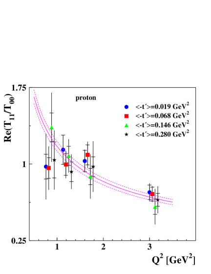
Refer to caption
Refer to caption
Figure 4: The Q2superscript𝑄2Q^{2} dependence of Re(T11/T00)Resubscript𝑇11subscript𝑇00\mathrm{Re}(T_{11}/T_{00}) for proton (left panel) and deuteron (right panel) data, showing the result for the 16 (Q2superscript𝑄2Q^{2}, tsuperscript𝑡-t^{\prime}) bins. Inner error bars show the statistical uncertainty and the total error bars represent statistical and systematic uncertainties added in quadrature. The parameterization of the curves is given by Eq. (66) and their parameters are given in Tab. 4. Central lines are calculated with the fitted values of parameters, while the dashed lines correspond to one standard deviation of the curve parameter. Except for the second tsuperscript𝑡-t^{\prime} bin, the data points are shifted for better visibility.
Refer to caption
Refer to caption
Figure 5: The Q2superscript𝑄2Q^{2} dependence of Re(T11/T00)Resubscript𝑇11subscript𝑇00\mathrm{Re}(T_{11}/T_{00}) (left panel) and Im(T11/T00)Imsubscript𝑇11subscript𝑇00\mathrm{Im}(T_{11}/T_{00}) (right panel) for proton and deuteron data. Points show the amplitude ratios from Tabs. 2 and 3 after averaging over four tsuperscript𝑡-t^{\prime} bins using Eqs. (67) and (68). The parameterization of the curves obtained from combined proton and deuteron data is given by Eqs. (66) and (69) while the parameters are given in Tab. 4. The meaning of the error bars and the explanation of the curves are the same as for Fig. 4. Here and hereafter proton data points are slightly displaced to the right for better visibility. As explained in the text, curves are shown as solid (dash-dotted) lines if the parameterization is based (not based) on pQCD predictions.
target ratio a𝑎a, GeV δa𝛿𝑎\delta a, GeV χ2/Ndfsuperscript𝜒2subscript𝑁𝑑𝑓\chi^{2}/N_{df}
proton Re(T11/T00)Resubscript𝑇11subscript𝑇00\mathrm{Re}(T_{11}/T_{00}) 1.173 ±0.048plus-or-minus0.048\pm 0.048 0.63
deuteron Re(T11/T00)Resubscript𝑇11subscript𝑇00\mathrm{Re}(T_{11}/T_{00}) 1.106 ±0.035plus-or-minus0.035\pm 0.035 1.04
proton+deuteron Re(T11/T00)Resubscript𝑇11subscript𝑇00\mathrm{Re}(T_{11}/T_{00}) 1.109 ±0.026plus-or-minus0.026\pm 0.026 0.78
target ratio b𝑏b, GeV-1 δb𝛿𝑏\delta b, GeV-1 χ2/Ndfsuperscript𝜒2subscript𝑁𝑑𝑓\chi^{2}/N_{df}
proton Im(T11/T00)Imsubscript𝑇11subscript𝑇00\mathrm{Im}(T_{11}/T_{00}) 0.340 ±0.025plus-or-minus0.025\pm 0.025 0.54
deuteron Im(T11/T00)Imsubscript𝑇11subscript𝑇00\mathrm{Im}(T_{11}/T_{00}) 0.359 ±0.020plus-or-minus0.020\pm 0.020 0.71
proton+deuteron Im(T11/T00)Imsubscript𝑇11subscript𝑇00\mathrm{Im}(T_{11}/T_{00}) 0.348 ±0.017plus-or-minus0.017\pm 0.017 0.75
Table 4: The Q2superscript𝑄2Q^{2} dependence of Re(T11/T00)Resubscript𝑇11subscript𝑇00\mathrm{Re}(T_{11}/T_{00}) and Im(T11/T00)Imsubscript𝑇11subscript𝑇00\mathrm{Im}(T_{11}/T_{00}) for proton, deuteron and combined data sets parameterized as given by Eqs. (66) and (69). The values of parameters with their total uncertainties are presented. The last column shows the value of χ2superscript𝜒2\chi^{2} per degree of freedom.

The dependences of the other amplitude ratios, which are described in the following, are examined in a similar manner as was done for Re(t11)Resubscript𝑡11\mathrm{Re}(t_{11}). In every case, it was checked that the respective four datasets containing 4 points each can be combined into one dataset containing 16 points. When proton and deuteron results are consistent, the data are combined and 32 points are used in the fit. All the fits to the Q2superscript𝑄2Q^{2} or tsuperscript𝑡t^{\prime} dependences use 16 data points for the proton or deuteron separately and 32 data points for the combined data sets. Only for the sake of a more clear representation of the kinematic dependence of amplitude ratios in one variable Q2superscript𝑄2Q^{2} (or tsuperscript𝑡t^{\prime}), we average the values of the amplitude ratios 𝒯=tλVλγ𝒯subscript𝑡subscript𝜆𝑉subscript𝜆𝛾\mathcal{T}=t_{\lambda_{V}\lambda_{\gamma}} or |u11|subscript𝑢11|u_{11}| over four tsuperscript𝑡-t^{\prime} (or Q2superscript𝑄2Q^{2}) bins at the same value of Q2superscript𝑄2Q^{2} (or tsuperscript𝑡t^{\prime}) using the standard relations for the mean value 𝒯delimited-⟨⟩𝒯\langle\mathcal{T}\rangle and squared total uncertainty (δ𝒯)2superscript𝛿𝒯2(\delta\mathcal{T})^{2}:

𝒯delimited-⟨⟩𝒯\displaystyle\langle\mathcal{T}\rangle =\displaystyle= j𝒯j/(σj)2m1/(σm)2,subscript𝑗subscript𝒯𝑗superscriptsubscript𝜎𝑗2subscript𝑚1superscriptsubscript𝜎𝑚2\displaystyle\frac{\sum_{j}\mathcal{T}_{j}/(\sigma_{j})^{2}}{\sum_{m}1/(\sigma_{m})^{2}}\;, (67)
(δ𝒯)2superscript𝛿𝒯2\displaystyle(\delta\mathcal{T})^{2} =\displaystyle= 1m1/(σm)2.1subscript𝑚1superscriptsubscript𝜎𝑚2\displaystyle\frac{1}{\sum_{m}1/(\sigma_{m})^{2}}\;. (68)

Here, σjsubscript𝜎𝑗\sigma_{j} denotes the total uncertainty of 𝒯jsubscript𝒯𝑗\mathcal{T}_{j} in the jthsuperscript𝑗𝑡j^{th} bin and δ𝒯𝛿𝒯\delta\mathcal{T} is the total uncertainty of the averaged ratio 𝒯𝒯\mathcal{T}. The same formula (68) is applied for the calculation of the statistical uncertainty δ𝒯stat𝛿subscript𝒯𝑠𝑡𝑎𝑡\delta\mathcal{T}_{stat} where σmsubscript𝜎𝑚\sigma_{m} is the statistical uncertainty of 𝒯msubscript𝒯𝑚\mathcal{T}_{m}.

In the left panel of Fig. 5, the average values of the ratio Re(t11)Resubscript𝑡11\mathrm{Re}(t_{11}) in each of the Q2superscript𝑄2Q^{2} bins for both the proton and deuteron targets are shown. As the results for the two targets are found to be compatible, a fit to the combined proton and deuteron data is performed and the result extracted for a𝑎a in Eq. (66) is also presented in Tab. 4. Reasonable values of χ2superscript𝜒2\chi^{2} per degree of freedom, χ2/Ndf1superscript𝜒2subscript𝑁𝑑𝑓1\chi^{2}/N_{df}\approx 1, are obtained. A comparison of the average values of ratio Re(t11)Resubscript𝑡11\mathrm{Re}(t_{11}) across tsuperscript𝑡-t^{\prime} bins and the curve calculated with Eq. (66) using the value of the parameter a𝑎a obtained from the combined proton and deuteron data is shown in the left panel of Fig. 5. The Q2superscript𝑄2Q^{2} dependence of Re(t11)Resubscript𝑡11\mathrm{Re}(t_{11}) is found to be in a good agreement with the asymptotic behavior expected from pQCD.

As shown in the right panel of Fig. 5, the amplitude ratio Im(t11)Imsubscript𝑡11\mathrm{Im}(t_{11}) rises with Q2superscript𝑄2Q^{2}. This dependence of Im(t11)Imsubscript𝑡11\mathrm{Im}(t_{11}) disagrees with the prediction IK ; KNZ given by Eq. (61), whereas the dependence of the real part of the same ratio t11subscript𝑡11t_{11} agrees with predictions based on the same formula. A fit of the function in Eq. (66) to the experimental data does not provide reasonable values of χ2superscript𝜒2\chi^{2} per degree of freedom: χ2/Ndf=2.46superscript𝜒2subscript𝑁𝑑𝑓2.46\chi^{2}/N_{df}=2.46 for the proton data and χ2/Ndf=4.25superscript𝜒2subscript𝑁𝑑𝑓4.25\chi^{2}/N_{df}=4.25 for the deuteron data. Instead, a fit function of the type

Im(t11)=bQImsubscript𝑡11𝑏𝑄\displaystyle\mathrm{Im}(t_{11})=bQ\; (69)

gives reasonable results as can be seen from Tab. 4, where fit results for the proton, deuteron and combined datasets are presented. The right panel of Fig. 5 shows the curve calculated with the parameter b𝑏b obtained for the combined proton and deuteron data compared with the tsuperscript𝑡-t^{\prime} bin averaged ratio Im(t11)Imsubscript𝑡11\mathrm{Im}(t_{11}) for both proton and deuteron data. The disagreement with the prediction of Eq. (61) may be due to the fact that the Q2superscript𝑄2Q^{2} range of the HERMES experiment is not in the asymptotic region. This is in agreement with the conjecture of Ref. KNZ that the hard scale for vector-meson electroproduction is QVsubscript𝑄𝑉Q_{V} given by Eq. (65) which is smaller than Q𝑄Q. Another possible explanation can be found in the discussion later in this paper of potential final-state interactions between the struck parton and the target remnant.

The phase difference δ11subscript𝛿11\delta_{11} between the helicity amplitudes T11subscript𝑇11T_{11} and T00subscript𝑇00T_{00} is given by the relation

tanδ11=Im(t11)/Re(t11).subscript𝛿11Imsubscript𝑡11Resubscript𝑡11\displaystyle\tan\delta_{11}=\mathrm{Im}(t_{11})/\mathrm{Re}(t_{11})\,. (70)

It increases with Q2superscript𝑄2Q^{2} as shown in the left panel of Fig. 6. Also shown is a fit to the Q2superscript𝑄2Q^{2} dependence of δ11subscript𝛿11\delta_{11} calculated with the functional form tan δ11=bQ2/asubscript𝛿11𝑏superscript𝑄2𝑎\delta_{11}=bQ^{2}/a deduced from Eqs. (66) and (69). The result of the fit is δ11=(31.5±1.4)subscript𝛿11plus-or-minus31.51.4\delta_{11}=(31.5\pm 1.4) degrees at Q2=1.95delimited-⟨⟩superscript𝑄21.95\langle Q^{2}\rangle=1.95 GeV2, obtained with the parameters a𝑎a and b𝑏b given in Tab. 4 for the combined proton and deuteron data. It is consistent within one standard deviation with the published result DC-24 obtained with the SDME method using the same proton and deuteron data as in the present analysis. A large phase difference δ1120subscript𝛿1120\delta_{11}\approx 20 degrees was measured by the H1 collaboration for exclusive ρ0superscript𝜌0\rho^{0} and ϕitalic-ϕ\phi meson electroproduction at 2.5 GeV<2Q2<60{}^{2}<Q^{2}<60 GeV2 H1-amp . A large value of δ11=(33.0±7.4)subscript𝛿11plus-or-minus33.07.4\delta_{11}=(33.0\pm 7.4) degrees was measured also in ϕitalic-ϕ\phi meson production at HERMES phi-sdmes . As two-gluon exchange dominates in ϕitalic-ϕ\phi meson production at HERMES kinematics, the measured large value of δ11subscript𝛿11\delta_{11} for ρ0superscript𝜌0\rho^{0} cannot be attributed solely to the quark-antiquark exchange essential for ρ0superscript𝜌0\rho^{0} meson production. This value of δ11subscript𝛿11\delta_{11} is in clear disagreement with a calculation  GK performed using a GPD-based approach in pQCD that predicts a very small value for δ11subscript𝛿11\delta_{11}. At present, there exists no model capable of explaining the value and Q2superscript𝑄2Q^{2} dependence of δ11subscript𝛿11\delta_{11}.

In existing pQCD calculations for exclusive vector-meson electroproduction, only two-gluon and/or quark-antiquark exchange have been taken into account. It can be argued Brodsky that even in inclusive deep-inelastic lepton-nucleon scattering, the final-state interaction of the struck quark alters the cross section due to multi-gluon exchanges with the target remnant. This is at variance with the traditional understanding obtained from inclusive DIS. It is shown Brodsky that a summation of multi-gluon-exchange amplitudes results in an eikonal-like correction. For vector-meson production, if rescattering on the nucleon occured also for the quark-antiquark pair that transforms to the final vector meson, the eikonal-like correction might be responsible for the measured large phases observed in the present work.
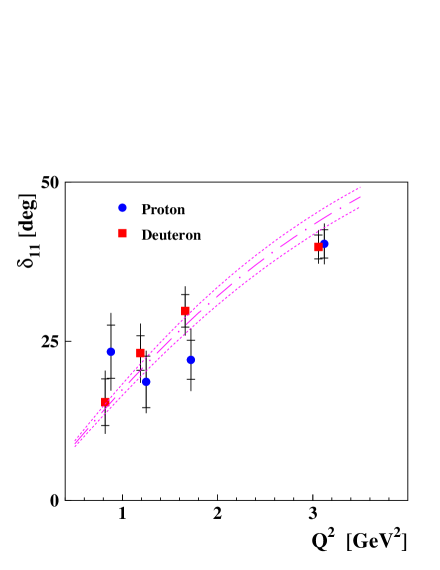
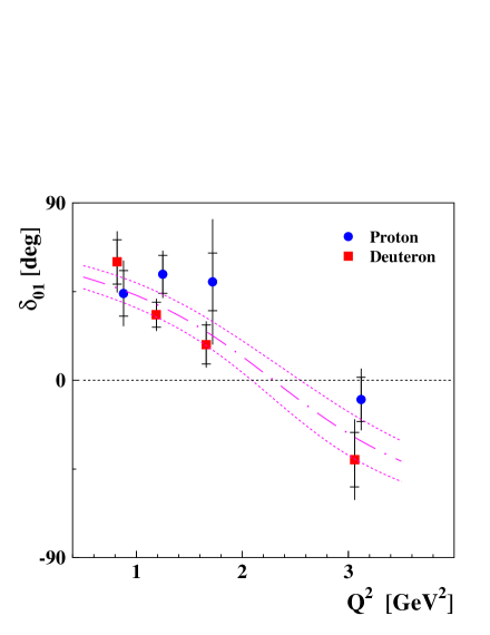
Refer to caption
Refer to caption
Figure 6: The Q2superscript𝑄2Q^{2} dependence of the phase difference δ11subscript𝛿11\delta_{11} (left panel) and δ01subscript𝛿01\delta_{01} (right panel, see Sec. 7.4) between the amplitudes T11subscript𝑇11T_{11} and T01subscript𝑇01T_{01}, respectively, and T00subscript𝑇00T_{00} obtained for proton and deuteron data. Points show the phase differences δ11subscript𝛿11\delta_{11} and δ01subscript𝛿01\delta_{01} calculated from ratios of amplitudes given in Tabs. 2 and 3 after averaging over tsuperscript𝑡-t^{\prime} bins. Inner error bars show the statistical uncertainty and the outer ones show the statistical and systematic uncertainties added in quadrature. The fitted parameterization is given by Eqs. (70) and (78) respectively for δ11subscript𝛿11\delta_{11} and δ01subscript𝛿01\delta_{01}. The parameters of the curves are given in Tabs. 4 and 6 for combined proton and deuteron data. The central lines are calculated with the fitted values of the parameters, while the dashed lines correspond to one standard deviation in the uncertainty of the curve parameter.
Refer to caption
Refer to caption
Figure 7: The tsuperscript𝑡t^{\prime} dependence of QRe(T11/T00)𝑄Resubscript𝑇11subscript𝑇00Q\cdot\mathrm{Re}(T_{11}/T_{00}) (left panel) and Im(T11/T00)/QImsubscript𝑇11subscript𝑇00𝑄\mathrm{Im}(T_{11}/T_{00})/Q (right panel) for proton and deuteron data. Points show the amplitude ratios from Tabs. 2 and 3 after averaging over four Q2superscript𝑄2Q^{2} bins using Eqs. (67) and (68). The straight lines in the left and right panel show the value of a𝑎a and b𝑏b, respectively, from Eqs. (66) and (69) while the parameters a𝑎a and b𝑏b are given in Tab. 4. The meaning of the error bars and the explanation of the curves are the same as for Fig. 4.
Refer to caption
Refer to caption
Figure 8: The dependences of |U11/T00|subscript𝑈11subscript𝑇00|U_{11}/T_{00}| on Q2superscript𝑄2Q^{2} and tsuperscript𝑡t^{\prime} for proton and deuteron data. The points show the amplitude ratios given in Tabs. 2 and 3 after averaging over tsuperscript𝑡-t^{\prime} (Q2superscript𝑄2Q^{2}) bins in the left (right) panel. The inner error bars show the statistical uncertainty and the outer ones show the statistical and systematic uncertainties added in quadrature. The results fitting the combined data set with a constant (central line), |U11/T00|=gsubscript𝑈11subscript𝑇00𝑔|U_{11}/T_{00}|=g, are given in Tab. 5. The dashed lines correspond to one standard deviation in the total uncertainty.
target ratio g𝑔g δg𝛿𝑔\delta g χ2/Ndfsuperscript𝜒2subscript𝑁𝑑𝑓\chi^{2}/N_{df}
proton |U11/T00|subscript𝑈11subscript𝑇00|U_{11}/T_{00}| 0.400 ±0.020plus-or-minus0.020\pm 0.020 0.60
deuteron |U11/T00|subscript𝑈11subscript𝑇00|U_{11}/T_{00}| 0.383 ±0.017plus-or-minus0.017\pm 0.017 0.40
proton+deuteron |U11/T00|subscript𝑈11subscript𝑇00|U_{11}/T_{00}| 0.390 ±0.013plus-or-minus0.013\pm 0.013 0.49
Table 5: Results of fitting the ratio |U11/T00|subscript𝑈11subscript𝑇00|U_{11}/T_{00}| to a constant for proton, deuteron and combined data sets. The values of parameters with their total uncertainties are presented. The last column shows the value of χ2superscript𝜒2\chi^{2} per degree of freedom.

Figure 7 shows the tsuperscript𝑡t^{\prime} dependence of the real and imaginary parts of the ratio t11subscript𝑡11t_{11}. Since Re(t11)Resubscript𝑡11\mathrm{Re}(t_{11}) and Im(t11)Imsubscript𝑡11\mathrm{Im}(t_{11}) depend on Q2superscript𝑄2Q^{2} according to Eqs. (66) and (69), they are shown in Fig. 7 multiplied or divided by Q𝑄Q, respectively. No noticeable tsuperscript𝑡t^{\prime} dependence is observed for Re(t11)Resubscript𝑡11\mathrm{Re}(t_{11}) and Im(t11)Imsubscript𝑡11\mathrm{Im}(t_{11}). Since the differential cross section of the process in Eq. (1) for high energies and small |t|superscript𝑡|t^{\prime}| is usually described by an exponential factor exp{βt}𝛽superscript𝑡\exp\{\beta t^{\prime}\}, the helicity amplitudes should have exponential factors T00exp{βLt/2}proportional-tosubscript𝑇00subscript𝛽𝐿superscript𝑡2T_{00}\propto\exp\{\beta_{L}t^{\prime}/2\} and T11exp{βTt/2}proportional-tosubscript𝑇11subscript𝛽𝑇superscript𝑡2T_{11}\propto\exp\{\beta_{T}t^{\prime}/2\}. The absence of a tsuperscript𝑡t^{\prime} dependence of the ratio T11/T00subscript𝑇11subscript𝑇00T_{11}/T_{00} means that the slope parameters βLsubscript𝛽𝐿\beta_{L} and βTsubscript𝛽𝑇\beta_{T} for the amplitudes T00subscript𝑇00T_{00} and T11subscript𝑇11T_{11} are close to each other. For very small |t|superscript𝑡|t^{\prime}|, it is reasonable to use the linear approximation

Re(T11/T00)Resubscript𝑇11subscript𝑇00\displaystyle\mathrm{Re}(T_{11}/T_{00}) =\displaystyle= aQexp{12Δβ1t}𝑎𝑄12Δsubscript𝛽1superscript𝑡\displaystyle\frac{a}{Q}\exp\{-\frac{1}{2}\Delta\beta_{1}t^{\prime}\}
\displaystyle\approx aQ(1+12Δβ1|t|),𝑎𝑄112Δsubscript𝛽1superscript𝑡\displaystyle\frac{a}{Q}(1+\frac{1}{2}\Delta\beta_{1}|t^{\prime}|), (71)
Im(T11/T00)Imsubscript𝑇11subscript𝑇00\displaystyle\mathrm{Im}(T_{11}/T_{00}) =\displaystyle= bQexp{12Δβ2t}𝑏𝑄12Δsubscript𝛽2superscript𝑡\displaystyle bQ\exp\{-\frac{1}{2}\Delta\beta_{2}t^{\prime}\}
\displaystyle\approx bQ(1+12Δβ2|t|).𝑏𝑄112Δsubscript𝛽2superscript𝑡\displaystyle bQ(1+\frac{1}{2}\Delta\beta_{2}|t^{\prime}|). (72)

The proton results are Δβ1=(1.02±0.85)Δsubscript𝛽1plus-or-minus1.020.85\Delta\beta_{1}=(-1.02\pm 0.85) GeV-2 and Δβ2=(0.91±2.00)Δsubscript𝛽2plus-or-minus0.912.00\Delta\beta_{2}=(-0.91\pm 2.00) GeV-2, while the fit for the deuteron data gives Δβ1=(0.58±0.80)Δsubscript𝛽1plus-or-minus0.580.80\Delta\beta_{1}=(0.58\pm 0.80) GeV-2 and Δβ2=(1.96±1.58)Δsubscript𝛽2plus-or-minus1.961.58\Delta\beta_{2}=(-1.96\pm 1.58) GeV-2. The results of the fits show that all four numbers are consistent with one another. We now assume that, within experimental accuracy, the slope parameters for the real and imaginary parts of the ratio coincide across both target types. In this case we have Δβ1Δβ2βLβTΔsubscript𝛽1Δsubscript𝛽2subscript𝛽𝐿subscript𝛽𝑇\Delta\beta_{1}\approx\Delta\beta_{2}\approx\beta_{L}-\beta_{T}. Combining these four numbers making use of Eqs. (67) and (68) we get an estimate for βLβT=(0.4±0.5)subscript𝛽𝐿subscript𝛽𝑇plus-or-minus0.40.5\beta_{L}-\beta_{T}=(-0.4\pm 0.5) GeV-2. This result on βLβTsubscript𝛽𝐿subscript𝛽𝑇\beta_{L}-\beta_{T} is in agreement with the prediction published in Ref. bzk , which ranges from 0.70.7-0.7 GeV-2 at Q2=0.8superscript𝑄20.8Q^{2}=0.8 GeV2 to 0.40.4-0.4 GeV-2 at Q2=5superscript𝑄25Q^{2}=5 GeV2.

target ratio c𝑐c, GeV-1 δc𝛿𝑐\delta c, GeV-1 χ2/Ndfsuperscript𝜒2subscript𝑁𝑑𝑓\chi^{2}/N_{df}
proton Re(T01/T00)Resubscript𝑇01subscript𝑇00\mathrm{Re}(T_{01}/T_{00}) 0.405 ±0.046plus-or-minus0.046\pm 0.046 0.56
deuteron Re(T01/T00)Resubscript𝑇01subscript𝑇00\mathrm{Re}(T_{01}/T_{00}) 0.378 ±0.033plus-or-minus0.033\pm 0.033 0.69
proton+deuteron Re(T01/T00)Resubscript𝑇01subscript𝑇00\mathrm{Re}(T_{01}/T_{00}) 0.394 ±0.024plus-or-minus0.024\pm 0.024 0.63
target ratio f𝑓f δf𝛿𝑓\delta f χ2/Ndfsuperscript𝜒2subscript𝑁𝑑𝑓\chi^{2}/N_{df}
proton Im(T01/T00)Imsubscript𝑇01subscript𝑇00\mathrm{Im}(T_{01}/T_{00}) 0.317 ±0.115plus-or-minus0.115\pm 0.115 0.97
deuteron Im(T01/T00)Imsubscript𝑇01subscript𝑇00\mathrm{Im}(T_{01}/T_{00}) 0.161 ±0.090plus-or-minus0.090\pm 0.090 1.20
proton+deuteron Im(T01/T00)Imsubscript𝑇01subscript𝑇00\mathrm{Im}(T_{01}/T_{00}) 0.221 ±0.069plus-or-minus0.069\pm 0.069 1.10
target ratio f1subscript𝑓1f_{1} GeV-1 δf1𝛿subscript𝑓1\delta f_{1} GeV-1 f2subscript𝑓2f_{2} GeV-3 δf2𝛿subscript𝑓2\delta f_{2} GeV-3 ρcsubscript𝜌𝑐\rho_{c} χ2/Ndfsuperscript𝜒2subscript𝑁𝑑𝑓\chi^{2}/N_{df}
proton+deuteron Im(T01/T00)Imsubscript𝑇01subscript𝑇00\mathrm{Im}(T_{01}/T_{00}) 0.653 ±0.132plus-or-minus0.132\pm 0.132 -0.285 ±0.065plus-or-minus0.065\pm 0.065 -0.903 0.66
Table 6: The kinematic dependence of Re(T01/T00)Resubscript𝑇01subscript𝑇00\mathrm{Re}(T_{01}/T_{00}) and Im(T01/T00)Imsubscript𝑇01subscript𝑇00\mathrm{Im}(T_{01}/T_{00}) for the proton, deuteron and combined data sets parameterized as given by Eqs. (7476)7476(\ref{fit-t/Q-Imt01}-\ref{fit-t-Ret01}). The values of parameters with their total uncertainties are presented. The last column shows the value of χ2superscript𝜒2\chi^{2} per degree of freedom and ρcsubscript𝜌𝑐\rho_{c} is the correlation parameter.

7.3 Kinematic Dependence of |U11/T00|subscript𝑈11subscript𝑇00|U_{11}/T_{00}|

The unnatural-parity-exchange amplitude, U11subscript𝑈11U_{11}, describes the transition from a transversely polarized photon to a transversely polarized ρ0superscript𝜌0\rho^{0} meson (γTρT0superscriptsubscript𝛾𝑇subscriptsuperscript𝜌0𝑇\gamma_{T}^{*}\rightarrow\rho^{0}_{T}). At large W𝑊W and Q2superscript𝑄2Q^{2}, this transition should be suppressed by a factor of MV/Qsubscript𝑀𝑉𝑄M_{V}/Q compared to the dominant amplitude T00subscript𝑇00T_{00} as explained in Sec. 4.2.2. The UPE contributions to the amplitude may be sizable at intermediate energies IW ; KS typical for HERMES.

The ratio |u11|subscript𝑢11|u_{11}| versus Q2superscript𝑄2Q^{2} and tsuperscript𝑡t^{\prime} is presented in Fig. 8. The value of |U11|subscript𝑈11|U_{11}| is found to be smaller than |T00|subscript𝑇00|T_{00}| by a factor of approximately 2.52.52.5. No kinematic dependences of the ratio |u11|subscript𝑢11|u_{11}| are seen and therefore it is fitted to a constant

|u11|=g.subscript𝑢11𝑔\displaystyle|u_{11}|=g. (73)

The results of the fit to proton and deuteron combined data are given in Tab. 5, and the constant g𝑔g is shown in Fig. 8 by straight lines. Fits with the same function a/Q𝑎𝑄a/Q as for Re(t11)Resubscript𝑡11\mathrm{Re}(t_{11}) (see Eq. (66)), corresponding to the behavior expected in pQCD, give values for χ2superscript𝜒2\chi^{2} per degree of freedom 2.032.032.03, 2.672.672.67, and 2.252.252.25 for the proton, deuteron, and combined data, respectively. This disagreement may reflect the fact that the HERMES Q2superscript𝑄2Q^{2} region is far from the asymptotic one.

From a study of soft hadron scattering, it is known IW ; KS ; Kaidalov that the most important contribution to UPE amplitudes at intermediate energies comes from pion exchange. The amplitude of one-pion-exchange in the t𝑡t-channel contains the propagator 1/(tmπ2)1𝑡superscriptsubscript𝑚𝜋21/(t-m_{\pi}^{2}), which become large for small values of t𝑡-t that approach the pole at the unphysical value of t=mπ20.018𝑡superscriptsubscript𝑚𝜋20.018-t=-m_{\pi}^{2}\approx-0.018 GeV2. The mean value of tsuperscript𝑡-t^{\prime} for the first tsuperscript𝑡-t^{\prime} bin is 0.019 GeV2, and hence might appear to be small enough to approach the vicinity of the pole. However, as shown in the right panel of Fig. 8, no evidence for a pion-pole-like dependence can be seen in the data within the statistical precision of the measurement. Such a dependence could be weakened by various effects:
i) even in the first bin in tsuperscript𝑡-t^{\prime}, the value of tdelimited-⟨⟩𝑡\langle-t\rangle equal to 0.060.060.06 GeV2 is substantial, and hence not close enough to the pion pole at unphysical positive t𝑡t,
ii) the amplitude T00subscript𝑇00T_{00} has a strong exponential dependence exp{βLt/2}proportional-toabsentsubscript𝛽𝐿superscript𝑡2\propto\exp\{\beta_{L}t^{\prime}/2\} with βL7subscript𝛽𝐿7\beta_{L}\approx 7 GeV-2 DC-24 ; tytgat and decreases with |t|superscript𝑡|t^{\prime}|, hence the ratio U11/T00subscript𝑈11subscript𝑇00U_{11}/T_{00} is flatter than U11subscript𝑈11U_{11} itself,
iii) in addition to one-pion exchange, other exchange processes can contribute to the amplitude U11subscript𝑈11U_{11}.

Using the amplitude method, the signal of unnatural-parity exchange has a significance of more than 20 standard deviations in the total experimental uncertainty separately for each of the proton and deuteron data sets (see Tab. 5 and Fig. 8). In contrast, the existence of UPE was established DC-24 with a significance of 3 standard deviations for the combined proton and deuteron data in the analysis using the SDME method.

7.4 Kinematic dependence of T01/T00subscript𝑇01subscript𝑇00T_{01}/T_{00}

The amplitude T01T012112subscript𝑇01subscript𝑇012112T_{01}\equiv T_{0\frac{1}{2}1\frac{1}{2}} describing the transition γTρL0superscriptsubscript𝛾𝑇subscriptsuperscript𝜌0𝐿\gamma_{T}^{*}\rightarrow\rho^{0}_{L} is expected to be the largest SCHC-violating amplitude. In accordance with the asymptotic formula (62), the parameterization

Im(t01)=ftQImsubscript𝑡01𝑓superscript𝑡𝑄\displaystyle\mathrm{Im}(t_{01})=f\frac{\sqrt{-t^{\prime}}}{Q} (74)

is used. A fit to both proton and deuteron data using this parameterization gives acceptable χ2superscript𝜒2\chi^{2} values, as seen in Tab. 6. Proton and deuteron results are compatible within one standard deviation in the total uncertainty, although neither measurement is particularly precise as shown in Tab. 6 and the right panel of Fig. 9 in which the data are multiplied by Q𝑄Q in order to demonstrate the tsuperscript𝑡\sqrt{-t^{\prime}} dependence. The fit of the combined proton and deuteron data set yields a value of the parameter f𝑓f that is three standard deviations from zero with χ2/Ndf0.66superscript𝜒2subscript𝑁𝑑𝑓0.66\chi^{2}/N_{df}\approx 0.66 (see Tab. 6). We note that these results do not necessarily confirm the validity of Eq. (62) although the data do not contradict the pQCD prediction.
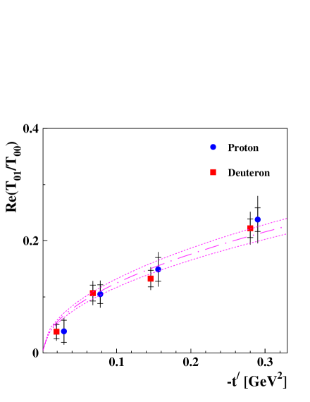
Refer to caption
Refer to caption
Figure 9: The tsuperscript𝑡t^{\prime} dependence of Re(T01/T00)Resubscript𝑇01subscript𝑇00\mathrm{Re}(T_{01}/T_{00}) (left panel) and QIm(T01/T00)𝑄Imsubscript𝑇01subscript𝑇00Q\cdot\mathrm{Im}(T_{01}/T_{00}) (right panel) for proton and deuteron data. Points show amplitude ratios from Tabs. 2 and 3 after averaging over Q2superscript𝑄2Q^{2} bins. Inner error bars show the statistical uncertainty and the outer bars show statistical and systematic uncertainties added in quadrature. The parameterization is given by Eqs. (74) and (76). The parameters of the curves are given in Tab. 6 for combined proton and deuteron data. Central lines are calculated with fitted values of parameters, while the dashed lines correspond to one standard deviation of the curve parameter.
Refer to caption
Refer to caption
Figure 10: The Q2superscript𝑄2Q^{2} dependence of Re(T01/T00)/tResubscript𝑇01subscript𝑇00superscript𝑡\mathrm{Re}(T_{01}/T_{00})/\sqrt{-t^{\prime}} (left panel) and Im(T01/T00)/tImsubscript𝑇01subscript𝑇00superscript𝑡\mathrm{Im}(T_{01}/T_{00})/\sqrt{-t^{\prime}} (right panel) for proton and deuteron data. Points show amplitude ratios from Tabs. 2 and 3 after averaging over tsuperscript𝑡-t^{\prime} bins. Inner error bars show the statistical uncertainty and the outer bars show statistical and systematic uncertainties added in quadrature. The parameterization is given by Eqs. (75) and (76). The parameters of the curves are given in Tab. 6 for combined proton and deuteron data. Central lines are calculated with fitted values of parameters, while the dashed lines correspond to one standard deviation of the curve parameter.

The Q2superscript𝑄2Q^{2} dependence of the amplitude ratio Im(t01)Imsubscript𝑡01\mathrm{Im}(t_{01}) for the proton and deuteron data is shown in the right panel of Fig. 10. As shown in the figure, the point for the deuteron in the largest Q2superscript𝑄2Q^{2} bin is slightly negative which favours a fit using the equation

Im(t01)=t(f1+f2Q2)Imsubscript𝑡01superscript𝑡subscript𝑓1subscript𝑓2superscript𝑄2\displaystyle\mathrm{Im}(t_{01})=\sqrt{-t^{\prime}}(f_{1}+f_{2}Q^{2}) (75)

over that using parameterization (74). The result of the fit with function (75) is shown in the right panel of Fig. 10. The parameters f1subscript𝑓1f_{1} and f2subscript𝑓2f_{2} are strongly correlated. The correlation parameter ρcsubscript𝜌𝑐\rho_{c} is presented in Tab. 6 and is taken into account in the calculation of the uncertainty of Im(t01)Imsubscript𝑡01\mathrm{Im}(t_{01}) using Eq. (75).

target ratio r𝑟r, GeV-1 δr𝛿𝑟\delta r, GeV-1 χ2/Ndfsuperscript𝜒2subscript𝑁𝑑𝑓\chi^{2}/N_{df}
proton Re(T10/T00)Resubscript𝑇10subscript𝑇00\mathrm{Re}(T_{10}/T_{00}) -0.012 ±0.030plus-or-minus0.030\pm 0.030 1.07
proton Im(T10/T00)Imsubscript𝑇10subscript𝑇00\mathrm{Im}(T_{10}/T_{00}) 0.019 ±0.061plus-or-minus0.061\pm 0.061 0.58
target ratio s𝑠s, GeV-3 δs𝛿𝑠\delta s, GeV-3 χ2/Ndfsuperscript𝜒2subscript𝑁𝑑𝑓\chi^{2}/N_{df}
deuteron Re(T10/T00)Resubscript𝑇10subscript𝑇00\mathrm{Re}(T_{10}/T_{00}) 0.045 ±0.015plus-or-minus0.015\pm 0.015 0.32
deuteron Im(T10/T00)Imsubscript𝑇10subscript𝑇00\mathrm{Im}(T_{10}/T_{00}) -0.109 ±0.021plus-or-minus0.021\pm 0.021 1.02
Table 7: The kinematic dependences of Re(T10/T00)Resubscript𝑇10subscript𝑇00\mathrm{Re}(T_{10}/T_{00}) and Im(T10/T00)Imsubscript𝑇10subscript𝑇00\mathrm{Im}(T_{10}/T_{00}) for proton and deuteron parameterized as given by Eqs. (79) and (80). The values of parameters with their total uncertainties are presented. The last column shows the value of χ2superscript𝜒2\chi^{2} per degree of freedom.
target ratio hh, GeV-1 δh𝛿\delta h, GeV-1 χ2/Ndfsuperscript𝜒2subscript𝑁𝑑𝑓\chi^{2}/N_{df}
proton+deuteron Re(T11/T00)Resubscript𝑇11subscript𝑇00\mathrm{Re}(T_{1-1}/T_{00}) -0.156 ±0.059plus-or-minus0.059\pm 0.059 0.79
proton+deuteron Im(T11/T00)Imsubscript𝑇11subscript𝑇00\mathrm{Im}(T_{1-1}/T_{00}) -0.418 ±0.126plus-or-minus0.126\pm 0.126 0.54
Table 8: The kinematic dependence of Re(T11/T00)Resubscript𝑇11subscript𝑇00\mathrm{Re}(T_{1-1}/T_{00}) and Im(T11/T00)Imsubscript𝑇11subscript𝑇00\mathrm{Im}(T_{1-1}/T_{00}) for combined proton and deuteron data parameterized as given by Eq. (83). The values of parameters with their total uncertainties are presented. The last column shows the value of χ2superscript𝜒2\chi^{2} per degree of freedom.

The Q2superscript𝑄2Q^{2} dependence of the ratio Re(t01)/tResubscript𝑡01superscript𝑡\mathrm{Re}(t_{01})/\sqrt{-t^{\prime}} is presented in the left panel of Fig. 10. The quantity Re(t01)Resubscript𝑡01\mathrm{Re}(t_{01})
/tabsentsuperscript𝑡/\sqrt{-t^{\prime}} does not decrease with Q2superscript𝑄2Q^{2} and can be well described by a constant which is also shown in the figure. Using for Re(t01)Resubscript𝑡01\mathrm{Re}(t_{01}) the functional form of Eq. (74) yields χ2/Ndfsuperscript𝜒2subscript𝑁𝑑𝑓\chi^{2}/N_{df} values of 1.081.081.08, 1.551.551.55, and 1.311.311.31 for separate fits to the proton, deuteron and combined data sets. Using instead the simpler parameterization

Re(t01)=ctResubscript𝑡01𝑐superscript𝑡\displaystyle\mathrm{Re}(t_{01})=c\sqrt{-t^{\prime}} (76)

decreases the value of χ2superscript𝜒2\chi^{2} by a factor of approximately two, indicating a better description of the data. The results of this fit are shown in Tab. 6 and the left panels of Figs. 9 and 10. The small values of χ2/Ndfsuperscript𝜒2subscript𝑁𝑑𝑓\chi^{2}/N_{df} as shown in Tab. 6 indicate that our systematic uncertainty might be overestimated.

The phase difference δ01subscript𝛿01\delta_{01} between the amplitudes T01subscript𝑇01T_{01} and T00subscript𝑇00T_{00} can be calculated using the formula

tanδ01=Im(t10)/Re(t10).subscript𝛿01Imsubscript𝑡10Resubscript𝑡10\displaystyle\tan\delta_{01}=\mathrm{Im}(t_{10})/\mathrm{Re}(t_{10}). (77)

The results for the Q2superscript𝑄2Q^{2} dependence of δ01subscript𝛿01\delta_{01} after averaging over tsuperscript𝑡-t^{\prime} bins are shown in the right panel of Fig. 6. The phase difference δ01subscript𝛿01\delta_{01} is non-zero and decreases with Q2superscript𝑄2Q^{2}. It is slightly negative for the deuteron data at the largest value of Q2superscript𝑄2Q^{2}. Using instead the results from the fits to formulas (75, 76) given in Tab. 6, the phase difference is obtained as

tanδ01=(f1+f2Q2)/c,subscript𝛿01subscript𝑓1subscript𝑓2superscript𝑄2𝑐\displaystyle\tan\delta_{01}=(f_{1}+f_{2}Q^{2})/c\;, (78)

which is shown as a curve in the right panel of Fig. 6. As can be seen, the fit function (78) is able to describes the Q2superscript𝑄2Q^{2} dependence of the phase difference δ01subscript𝛿01\delta_{01}.

7.5 Small Amplitude Ratios T10/T00subscript𝑇10subscript𝑇00T_{10}/T_{00} and T11/T00subscript𝑇11subscript𝑇00T_{1-1}/T_{00}

According to the hierarchy given in Eq. (31), T10subscript𝑇10T_{10} and T11subscript𝑇11T_{1-1} are the smallest amplitudes that give linear contributions to the numerators of SDMEs in the case of an unpolarized target. The ratio t10subscript𝑡10t_{10} is expected to be proportional to tsuperscript𝑡\sqrt{-t^{\prime}} in accordance with Eq. (60), while t11subscript𝑡11t_{1-1} is expected to be proportional to tsuperscript𝑡t^{\prime}. These ratios are supposed to depend on Q2superscript𝑄2Q^{2} in the asymptotic region according to Eqs. (63) and (64). Figure 11 shows Re(t10)/tResubscript𝑡10superscript𝑡\mathrm{Re}(t_{10})/\sqrt{-t^{\prime}} and Im(t10)/tImsubscript𝑡10superscript𝑡\mathrm{Im}(t_{10})/\sqrt{-t^{\prime}} versus Q2superscript𝑄2Q^{2} for both proton and deuteron data. As shown in Fig. 11, the values of Re(t10)/tResubscript𝑡10superscript𝑡\mathrm{Re}(t_{10})/\sqrt{-t^{\prime}} and Im(t10)/tImsubscript𝑡10superscript𝑡\mathrm{Im}(t_{10})/\sqrt{-t^{\prime}} on the proton are compatible with zero. The results of the fit of Re(t10)Resubscript𝑡10\mathrm{Re}(t_{10}) with the function

Re(t10)=rtResubscript𝑡10𝑟superscript𝑡\displaystyle\mathrm{Re}(t_{10})=r\sqrt{-t^{\prime}} (79)

and Im(t10)Imsubscript𝑡10\mathrm{Im}(t_{10}) with the same function are presented in Tab. 7. The ratio Re(t10)/tResubscript𝑡10superscript𝑡\mathrm{Re}(t_{10})/\sqrt{-t^{\prime}} for the deuteron is slightly positive (except the first point at the smallest value of Q2superscript𝑄2Q^{2}) and increases with Q2superscript𝑄2Q^{2}. The fit of the deuteron data with the function

Re(t10)=sQ2tResubscript𝑡10𝑠superscript𝑄2superscript𝑡\displaystyle\mathrm{Re}(t_{10})=sQ^{2}\sqrt{-t^{\prime}} (80)

provides the positive result which is presented in Tab. 7. As shown in Fig. 11, the quantity Im(t10)/tImsubscript𝑡10superscript𝑡\mathrm{Im}(t_{10})/\sqrt{-t^{\prime}} is negative for the three points at the largest values of Q2superscript𝑄2Q^{2}. The fit of Im(t10)/tImsubscript𝑡10superscript𝑡\mathrm{Im}(t_{10})/\sqrt{-t^{\prime}} using the same function (80) gives the negative result presented in Tab. 7. This behavior contradicts the pQCD prediction given by Eq. (63), and indicates that in the case of the amplitude T10subscript𝑇10T_{10} the HERMES kinematic range may be far from the large-Q𝑄Q asymptotic region.

We recall that the amplitudes T00subscript𝑇00T_{00} and T10subscript𝑇10T_{10} vanish in the small Q𝑄Q-limit (Q20superscript𝑄20Q^{2}\rightarrow 0) because the real photon has no longitudinal polarization. If the behavior at fixed tsuperscript𝑡t^{\prime} and small Q2superscript𝑄2Q^{2} were described by

T00subscript𝑇00\displaystyle T_{00} proportional-to\displaystyle\propto Q,𝑄\displaystyle Q\;, (81)
T10subscript𝑇10\displaystyle T_{10} proportional-to\displaystyle\propto Q3,superscript𝑄3\displaystyle Q^{3}, (82)

the behavior of the ratio t10T10/T00subscript𝑡10subscript𝑇10subscript𝑇00t_{10}\equiv T_{10}/T_{00} would be just as assumed by Eq. (80) and presented in Fig. 11.
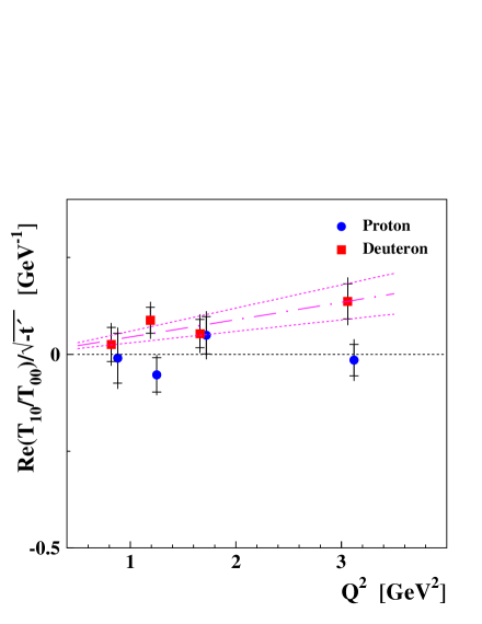
Refer to caption
Refer to caption
Figure 11: The Q2superscript𝑄2Q^{2} dependence of Re(T10/T00)/tResubscript𝑇10subscript𝑇00superscript𝑡\mathrm{Re}(T_{10}/T_{00})/\sqrt{-t^{\prime}} (left panel) and Im(T10/T00)/tImsubscript𝑇10subscript𝑇00superscript𝑡\mathrm{Im}(T_{10}/T_{00})/\sqrt{-t^{\prime}} (right panel) for proton and deuteron data. Points show amplitude ratios from Tabs. 2 and 3 after averaging over tsuperscript𝑡-t^{\prime} bins. Inner error bars show the statistical uncertainty and the outer ones indicate statistical and systematic uncertainties added in quadrature. The parameterization of the curves describing the deuteron data both on Re(T10/T00)Resubscript𝑇10subscript𝑇00\mathrm{Re}(T_{10}/T_{00}) and Im(T10/T00)Imsubscript𝑇10subscript𝑇00\mathrm{Im}(T_{10}/T_{00}) is given by Eq. (80) and their parameters are given in Tab. 7. Central lines are calculated with the fitted values of parameters, while the dashed lines correspond to one standard deviation of the curve parameter.
Refer to caption
Refer to caption
Figure 12: The Q2superscript𝑄2Q^{2} dependence of Re(T11/T00)/(t)Resubscript𝑇11subscript𝑇00superscript𝑡\mathrm{Re}(T_{1-1}/T_{00})/(-t^{\prime}) (left panel) and Im(T11/T00)/(t)Imsubscript𝑇11subscript𝑇00superscript𝑡\mathrm{Im}(T_{1-1}/T_{00})/(-t^{\prime}) (right panel) for proton and deuteron data. Points show amplitude ratios from Tabs. 2 and 3 after averaging over tsuperscript𝑡-t^{\prime} bins. Inner error bars show the statistical uncertainty and the outer ones indicate statistical and systematic uncertainties added in quadrature. The parameterization of the curves describing the combined proton and deuteron data both on Re(T11/T00)Resubscript𝑇11subscript𝑇00\mathrm{Re}(T_{1-1}/T_{00}) and Im(T11/T00)Imsubscript𝑇11subscript𝑇00\mathrm{Im}(T_{1-1}/T_{00}) is given by Eq. (83) and their parameters are given in Tab. 8. Central lines are calculated with the fitted values of parameters, while the dashed lines correspond to one standard deviation of the curve parameter.
Refer to caption
Refer to caption
Figure 13: The kinematic dependences of Re(T11/T00)Resubscript𝑇11subscript𝑇00\mathrm{Re}(T_{11}/T_{00}) and Re(T01/T00)Resubscript𝑇01subscript𝑇00\mathrm{Re}(T_{01}/T_{00}) for proton and deuteron data. Points of HERMES are the same as in Figs. 5 and 9. The H1 results are from Ref. H1-amp . Inner error bars show the statistical uncertainty and the outer ones indicate statistical and systematic uncertainties added in quadrature.

The ratios Re(t11)/(t)Resubscript𝑡11superscript𝑡\mathrm{Re}(t_{1-1})/(-t^{\prime}) and Im(t11)/(t)Imsubscript𝑡11superscript𝑡\mathrm{Im}(t_{1-1})/(-t^{\prime}) are presented versus Q2superscript𝑄2Q^{2} in Fig. 12. Both ratios appear to be compatible with zero within 2.52.52.5 σ𝜎\sigma of the total uncertainty both for the proton and deuteron target and only the combined data provides a non-zero signal for Im(t11)Imsubscript𝑡11\mathrm{Im}(t_{1-1}). The fit of Re(t11)Resubscript𝑡11\mathrm{Re}(t_{1-1}) with the function

Re(t11)=(t)hQResubscript𝑡11superscript𝑡𝑄\displaystyle\mathrm{Re}(t_{1-1})=(-t^{\prime})\frac{h}{Q} (83)

corresponds to the second term in Eq. (64). The result, presented in Tab. 8 for the combined proton and deuteron data, shows a signal of 2σ2𝜎2\sigma significance with respect to the total uncertainty. The result of the fit of Im(t11)Imsubscript𝑡11\mathrm{Im}(t_{1-1}) with the same function (83) is also presented in Tab. 8. The parameter hh deviates from zero by more than three standard deviations of the total uncertainty. A fit of the combined proton and deuteron data with both terms in Eq. (64) provides values of C1subscript𝐶1C_{1} and C2subscript𝐶2C_{2} that are consistent with zero within 1.51.51.5 σ𝜎\sigma of the total uncertainty for both Re(t11)Resubscript𝑡11\mathrm{Re}(t_{1-1}) and Im(t11)Imsubscript𝑡11\mathrm{Im}(t_{1-1}). This means that the statistical precision of the HERMES data does not allow a reliable verification of Eq. (64) or an extraction of the gluon transversity GPD.

7.6 Comparison of HERMES and H1 Results

Here we compare the results of the present work with the analysis of the ρ0superscript𝜌0\rho^{0}-meson production data on the proton by the H1 collaboration H1-amp , obtained for the CM energy range 363636 GeV W180absent𝑊180\leq W\leq 180 GeV, photon virtuality 2.52.52.5 GeV2 Q260absentsuperscript𝑄260\leq Q^{2}\leq 60 GeV2, and t3superscript𝑡3-t^{\prime}\leq 3 GeV2. For the comparison of the tsuperscript𝑡t^{\prime} dependence, the results at the mean value of Q2superscript𝑄2Q^{2} equal to 3.3 GeV2 are chosen which are the closest ones to the Q2superscript𝑄2Q^{2} region of the HERMES data. In the H1 data analysis presented in Ref. H1-amp , the imaginary parts of the amplitude ratios were not extracted. The additional hypothesis was used in Ref. H1-amp that for any ratio of the amplitudes, the approximate relation |tλVλγ|2=[Re(tλVλγ)]2superscriptsubscript𝑡subscript𝜆𝑉subscript𝜆𝛾2superscriptdelimited-[]Resubscript𝑡subscript𝜆𝑉subscript𝜆𝛾2|t_{\lambda_{V}\lambda_{\gamma}}|^{2}=[\mathrm{Re}(t_{\lambda_{V}\lambda_{\gamma}})]^{2} is valid within the experimental accuracy. The comparison of the HERMES and H1 results is presented in Fig. 13. As seen from the figure the HERMES and H1 results agree within their total uncertainties. No strong dependence on W𝑊W is observed for the amplitude ratios Re(t11)Resubscript𝑡11\mathrm{Re}(t_{11}) and Re(t01)Resubscript𝑡01\mathrm{Re}(t_{01}). Considering the differences in Q2superscript𝑄2Q^{2} between HERMES (Q2=2.0delimited-⟨⟩superscript𝑄22.0\langle Q^{2}\rangle=2.0 GeV2) and H1 (Q2=3.3delimited-⟨⟩superscript𝑄23.3\langle Q^{2}\rangle=3.3 GeV2), no Q2superscript𝑄2Q^{2} dependence can be seen for Re(t01)Resubscript𝑡01\mathrm{Re}(t_{01}) at small |t|superscript𝑡|t^{\prime}| even for Q23.3superscript𝑄23.3Q^{2}\leq 3.3 GeV2 (see also the discussion in Sec. 7.4). The ratios Re(t10)Resubscript𝑡10\mathrm{Re}(t_{10}) and Re(t11)Resubscript𝑡11\mathrm{Re}(t_{1-1}) obtained by H1 H1-amp are compatible with zero at Q2=3.1superscript𝑄23.1Q^{2}=3.1 GeV2 within the experimental accuracy. This is consistent with the HERMES results for the proton shown in Figs. 11 and 12.

8 Conclusions

Exclusive ρ0superscript𝜌0\rho^{0}-meson electroproduction is studied in the HERMES experiment, using a 27.627.627.6 GeV longitudinally polarized electron/positron beam and unpolarized hydrogen and deuterium targets in the kinematic region 0.50.50.5 GeV<2Q2<7.0{}^{2}<Q^{2}<7.0 GeV2, 3.03.03.0 GeV <W<6.3absent𝑊6.3<W<6.3 GeV, and t<0.4superscript𝑡0.4-t^{\prime}<0.4 GeV2. These data are used to determine the real and imaginary parts of the ratios T11/T00subscript𝑇11subscript𝑇00T_{11}/T_{00}, T01/T00subscript𝑇01subscript𝑇00T_{01}/T_{00}, T10/T00subscript𝑇10subscript𝑇00T_{10}/T_{00}, T11/T00subscript𝑇11subscript𝑇00T_{1-1}/T_{00}, and |U11/T00|subscript𝑈11subscript𝑇00|U_{11}/T_{00}| for 16 bins in Q2superscript𝑄2Q^{2} and tsuperscript𝑡-t^{\prime}. Systematic uncertainties due to the background contribution, uncertainties in the Monte Carlo input parameters, and the uncertainty of the applied amplitude method are given. Except for T10/T00subscript𝑇10subscript𝑇00T_{10}/T_{00}, the amplitude ratios for the proton are compatible with those for the deuteron. The extracted amplitude ratios T11/T00subscript𝑇11subscript𝑇00T_{11}/T_{00}, |U11/T00|subscript𝑈11subscript𝑇00|U_{11}/T_{00}| and T01/T00subscript𝑇01subscript𝑇00T_{01}/T_{00} are found to be sizable. The ratios T10/T00subscript𝑇10subscript𝑇00T_{10}/T_{00} and T11/T00subscript𝑇11subscript𝑇00T_{1-1}/T_{00} for the proton are found to be compatible with zero within experimental uncertainties. The ratio T11/T00subscript𝑇11subscript𝑇00T_{1-1}/T_{00} for the deuteron is also zero within experimental accuracy, while Re(T10/T00)Resubscript𝑇10subscript𝑇00\mathrm{Re}(T_{10}/T_{00}) is slightly positive and Im(T10/T00)Imsubscript𝑇10subscript𝑇00\mathrm{Im}(T_{10}/T_{00}) is slightly negative, except for the bin with the smallest Q2superscript𝑄2Q^{2} values.

The SDMEs calculated in terms of these helicity amplitude ratios generally agree with the results published in Ref. DC-24 . The amplitude method was shown to provide more accurate polarized SDMEs than the previous analysis using the SDME method.

The statistical precision available in this analysis permits the parameterization of the kinematic dependences of amplitude ratios and the extraction of the phase difference between various helicity amplitudes. The real part of T11/T00subscript𝑇11subscript𝑇00T_{11}/T_{00} is found to follow the asymptotic 1/Q1𝑄1/Q behavior predicted by pQCD IK ; KNZ . The imaginary part of T11/T00subscript𝑇11subscript𝑇00T_{11}/T_{00} grows with Q2superscript𝑄2Q^{2}, in contradiction to the large-Q2superscript𝑄2Q^{2} asymptotic behavior expected from pQCD. The phase difference δ11subscript𝛿11\delta_{11} between the amplitudes T11subscript𝑇11T_{11} and T00subscript𝑇00T_{00} grows with Q2superscript𝑄2Q^{2} and has a mean value of about 30 degrees in the HERMES kinematic region. This is in agreement with the published result of the SDME method DC-24 and in contradiction to calculations golos1 ; golos2 ; golos3 ; IK ; KNZ based on pQCD. For the first time, the Q2superscript𝑄2Q^{2} dependence of δ11subscript𝛿11\delta_{11} observed in Ref. DC-24 is shown to be related to the increase with Q2superscript𝑄2Q^{2} of the imaginary part of the ratio of the helicity amplitudes T11/T00subscript𝑇11subscript𝑇00T_{11}/T_{00}.

The behavior of Im(T01/T00)Imsubscript𝑇01subscript𝑇00\mathrm{Im}(T_{01}/T_{00}) is found to be in agreement with the asymptotic pQCD behavior t/Qsuperscript𝑡𝑄\sqrt{-t^{\prime}}/Q, while the extracted value of Re(T01/T00)Resubscript𝑇01subscript𝑇00\mathrm{Re}(T_{01}/T_{00}) is likely to be in disagreement with the pQCD prediction. The data indicate non-zero values of the phase difference δ01subscript𝛿01\delta_{01} between the amplitudes T01subscript𝑇01T_{01} and T00subscript𝑇00T_{00} and the decrease of δ01subscript𝛿01\delta_{01} with Q2superscript𝑄2Q^{2}.

The ratio |U11/T00|subscript𝑈11subscript𝑇00|U_{11}/T_{00}| is found to be constant in the HERMES kinematic region, in disagreement with the asymptotic pQCD behavior at large Q2superscript𝑄2Q^{2}. No pion-pole-like behavior is observed at small |t|superscript𝑡|t^{\prime}|. The UPE signal is seen with a very high significance for both proton and deuteron data, confirming the existence of unnatural-parity exchange contributions with a higher precision than that obtained with the SDME method DC-24 .

The Q2superscript𝑄2Q^{2} dependence of the amplitude ratio Re(T11/T00)Resubscript𝑇11subscript𝑇00\mathrm{Re}(T_{11}/T_{00}) and tsuperscript𝑡t^{\prime} dependence of the amplitude ratio Re(T01/T00)Resubscript𝑇01subscript𝑇00\mathrm{Re}(T_{01}/T_{00}) are also compared to those extracted by the H1 collaboration at the center-of-mass energy range 363636 GeV W180absent𝑊180\leq W\leq 180 GeV, photon virtuality 2.52.52.5 GeV2Q260{}^{2}\leq Q^{2}\leq 60 GeV2, and t3superscript𝑡3-t^{\prime}\leq 3 GeV2. No strong dependence of the amplitude ratios Re(T11/T00)Resubscript𝑇11subscript𝑇00\mathrm{Re}(T_{11}/T_{00}) and Re(T01/T00)Resubscript𝑇01subscript𝑇00\mathrm{Re}(T_{01}/T_{00}) on W𝑊W, and no Q2superscript𝑄2Q^{2} dependence of Re(t01)Resubscript𝑡01\mathrm{Re}(t_{01}) at small |t|superscript𝑡|t^{\prime}| are observed. The HERMES and H1 results agree within their total uncertainties.

Acknowledgments

We would like to thank M. Diehl, S.V. Goloskokov, P. Hoyer, and P. Kroll for many useful discussions.

We gratefully acknowledge the DESYmanagement for its support and the staff at DESY and the collaborating institutions for their significant effort. This work was supported by the Ministry of Economy and the Ministry of Education and Science of Armenia; the FWO-Flanders and IWT, Belgium; the Natural Sciences and Engineering Research Council of Canada; the National Natural Science Foundation of China; the Alexander von Humboldt Stiftung, the German Bundesministerium für Bildung und Forschung (BMBF), and the Deutsche Forschungsgemeinschaft (DFG); the Italian Istituto Nazionale di Fisica Nucleare (INFN); the MEXT, JSPS, and G-COE of Japan; the Dutch Foundation for Fundamenteel Onderzoek der Materie (FOM); the Russian Academy of Science and the Russian Federal Agency for Science and Innovations; the U.K. Engineering and Physical Sciences Research Council, the Science and Technology Facilities Council, and the Scottish Universities Physics Alliance; and the U.S. Department of Energy (DOE) and the National Science Foundation (NSF).

References

  • (1) T. H. Bauer, R. D. Spital, D. R. Yenni and F. M. Pipkin, Rev. Mod. Phys. 50, 261 (1978).
  • (2) I. P. Ivanov, N. N. Nikolaev, A. A. Savin, Phys. Part. Nucl. 37, 1 (2006).
  • (3) K. Schilling, G. Wolf, Nucl. Phys. B 61, 381 (1973).
  • (4) H. Fraas, Ann. Phys. 87, 417 (1974).
  • (5) M. Diehl, JHEP 0709, 064 (2007).
  • (6) D. Müller et al., Fortschr. Phys. 42, 101 (1994).
  • (7) X. Ji, Phys. Rev. Lett. 78, 610 (1997); Phys. Rev. D 55, 7114 (1997).
  • (8) A. V. Radyushkin, Phys. Rev. D 56, 5524 (1997).
  • (9) M. Diehl, Phys. Rep. 388, 41 (2003).
  • (10) A. V. Belitsky, A. V. Radyushkin, Phys. Rep. 418, 1 (2005).
  • (11) S. V. Goloskokov and P. Kroll, Eur. Phys. J. C 42, 02298 (2005).
  • (12) S. V. Goloskokov and P. Kroll, Eur. Phys. J. C 50, 829 (2007).
  • (13) S. V. Goloskokov and P. Kroll, Eur. Phys. J. C 53, 367 (2008).
  • (14) B. M. Vanderhaegen, P. A. M. Guichon, M. Guidal, Phys. Rev. Lett. 80, 5064 (1998).
  • (15) C. G. Goeke, M. V. Polyakov, M. Vanderhaegen, Prog. Part. Nucl. Phys. 47, 401 (2001).
  • (16) D. M. Guidal, M. V. Polyakov, A. V. Radyushkin, M. Vanderhaegen, Phys. Rev. D72, 054013 (2005).
  • (17) J. C. Collins, L. Frankfurt and M. Strikman, Phys. Rev. D 56, 2982 (1997).
  • (18) A. Airapetian et al. (HERMES Collaboration), Eur. Phys. J. C 62, 659 (2009).
  • (19) S. Chekanov et al. (ZEUS Collaboration), PMC Phys. A 1, 6 (2007).
  • (20) F. D. Aaron et al. (H1 Collaboration), JHEP 1005, 32 (2010).
  • (21) M. Derrick et al. (ZEUS Collaboration), Phys. Lett. B 380, 220 (1996).
  • (22) J. Breitweg et al. (ZEUS Collaboration), Eur. Phys. J. C 6, 603 (1999).
  • (23) C. Adloff et al. (H1 Collaboration), Phys. Lett. B 483, 360 (2000).
  • (24) C. Adloff et al. (H1 Collaboration), Eur. Phys. J. C 13, 371 (2000).
  • (25) S. Aid et al. (H1 Collaboration), Nucl. Phys. B 468, 3 (1996).
  • (26) M. R. Adams et al. (E665 Collaboration), Z. Phys. C 74, 237 (1997).
  • (27) A. Airapetian et al. (HERMES Collaboration), Eur. Phys. J. C 17, 389 (2000).
  • (28) C. Hadjidakis et al. (CLAS Collaboration), Phys. Lett. B 605, 256 (2005).
  • (29) S. A. Morrow et al. (CLAS Collaboration), Eur. Phys. J. A 39, 5 (2009).
  • (30) D. Yu. Ivanov and R. Kirschner, Phys. Rev. D 58, 114026 (1998).
  • (31) E. V. Kuraev, N. N. Nikolaev, and B. G. Zakharov, Pis’ma ZHETF 68, 667 (1998) (translation in JETP. Lett. 68, 696 (1998)).
  • (32) R. Kirschner, Nucl. Phys. B (Proc. Suppl.) 79, 340 (1999).
  • (33) N. Kivel, Phys. Rev. D 65, 054010 (2002).
  • (34) P. Joos et al., Nucl. Phys. B 113, 53 (1976).
  • (35) A. C. Irving, R. P. Worden, Phys. Rep. C 34, 117 (1977).
  • (36) G. L. Kane, A. Seidl. Rev. Mod. Phys. 48, Part I, 309 (1976).
  • (37) G. Cohen-Tannoudji, Ph. Salin, and A. Morel, Nuovo Cim. A 55, 412 (1968).
  • (38) M. N. Rosenbluth, Phys. Rev. 79, 615 (1950).
  • (39) J. Breitweg et al. (ZEUS Collaboration), Eur. Phys. J. C 12, 393 (2000).
  • (40) S. I. Manayenkov, Preprint PNPI 2856, Gatchina (2010).
  • (41) K. Ackerstaff et al. (HERMES Collaboration), Nucl. Instr. and Meth. A 417, 230 (1998).
  • (42) A. Sokolov and I. Ternov, Sov. Phys. Doklady 8, 1203 (1964).
  • (43) D. P. Barber et al., Nucl. Instr. and Meth. A 329, 79 (1993).
  • (44) M. Beckmann et al. (HERMES Collaboration), Nucl. Instr. and Meth. A 479, 334 (2002).
  • (45) N. Akopov et al., Nucl. Instr. and Meth. A 479, 511 (2002).
  • (46) K. Ackerstaff et al. (HERMES Collaboration), Eur. Phys. J. C 18, 303 (2000).
  • (47) M. Tytgat, Ph.D. Thesis, Gent University, DESY-THESIS-2001-014 (2001).
  • (48) A. A. Rostomyan, Ph.D. Thesis, Hamburg University, DESY-THESIS-2008-042 (2008).
  • (49) CERN-CN Division, CERN Program Library Long Writeup D 506 (1992).
  • (50) T. Sjöstrand, L. Lonnblad, S. Mrenna and P. Skands, PYTHIA 6.3: Physics and manual, hep-ph/0308153.
  • (51) W. Augustyniak, A. Borissov, S. Manayenkov, arXiv:0808.0669 (2008).
  • (52) S. V. Goloskokov, P. Kroll, Eur. Phys. J. C 59, 809 (2009).
  • (53) S.J. Brodsky, P. Hoyer, N. Marchal, S. Peigne and F. Sannino, Phys. Rev. D 65, 114025 (2002).
  • (54) B. Z. Kopeliovich, J. Nemchik and I. Schmidt, Phys. Rev. C 76, 025210 (2007).
  • (55) K. G. Boreskov, A. B. Kaidalov, O. V. Kancheli, Yad. Phys. 69, 1802 (2006).

Appendix A Systematic Uncertainty of the Amplitude Method for an Unpolarized Target

The systematic uncertainty arising from the neglect of amplitudes that make small contributions to the angular distribution applies if only data on unpolarized targets are considered. If the set of observables were enlarged and data on targets with transverse and longitudinal polarizations were added, then all the amplitude ratios could be extracted and there would be no contributory systematic uncertainty of the amplitude method.

The SDME analysis DC-24 of the HERMES data has shown the absence of any signal of the UPE amplitudes U01subscript𝑈01U_{01}, U10subscript𝑈10U_{10}, and U11subscript𝑈11U_{1-1}, violating the SCHC approximation. The contribution of the greatest UPE amplitude U11subscript𝑈11U_{11} to any SDME changes it by a value which is less or about one standard deviation of the statistical uncertainty. We neglect the contributions of U01subscript𝑈01U_{01}, U10subscript𝑈10U_{10}, and U11subscript𝑈11U_{1-1} to the SDMEs and do not consider that as a possible source of systematic uncertainty. The terms with the amplitudes U01subscript𝑈01U_{01}, U10subscript𝑈10U_{10}, and U11subscript𝑈11U_{1-1} in all the formulas considered in this appendix are also ignored. As explained in Sec. 4.2.1 the fractional contribution to SDMEs of NPE helicity-flip amplitudes are suppressed by α2superscript𝛼2\alpha^{2}. The systematic uncertainty of the extracted amplitude ratios due to the neglect of the NPE nucleon helicity-flip amplitudes is the only uncertainty of the amplitude method which is considered below.

The true ratio of the NPE amplitude without helicity flip TλV12λγ12subscript𝑇subscript𝜆𝑉12subscript𝜆𝛾12T_{\lambda_{V}\frac{1}{2}\lambda_{\gamma}\frac{1}{2}} to T012012subscript𝑇012012T_{0\frac{1}{2}0\frac{1}{2}} is denoted by tλVλγsubscript𝑡subscript𝜆𝑉subscript𝜆𝛾t_{\lambda_{V}\lambda_{\gamma}}. The true ratio of the nucleon-helicity-flip amplitude TλVλγsTλV12λγ12subscriptsuperscript𝑇𝑠subscript𝜆𝑉subscript𝜆𝛾subscript𝑇subscript𝜆𝑉12subscript𝜆𝛾12T^{s}_{\lambda_{V}\lambda_{\gamma}}\equiv T_{\lambda_{V}-\frac{1}{2}\lambda_{\gamma}\frac{1}{2}} to T012012subscript𝑇012012T_{0\frac{1}{2}0\frac{1}{2}} is denoted by tλVλγssubscriptsuperscript𝑡𝑠subscript𝜆𝑉subscript𝜆𝛾t^{s}_{\lambda_{V}\lambda_{\gamma}}, in particular, t00sT012012subscriptsuperscript𝑡𝑠00subscript𝑇012012t^{s}_{00}\equiv T_{0-\frac{1}{2}0\frac{1}{2}}
/T012012absentsubscript𝑇012012/T_{0\frac{1}{2}0\frac{1}{2}}, while |u11|2(|U112112|2+|U112112|2)/|T012012|2superscriptsubscript𝑢112superscriptsubscript𝑈1121122superscriptsubscript𝑈1121122superscriptsubscript𝑇0120122|u_{11}|^{2}\equiv(|U_{1\frac{1}{2}1\frac{1}{2}}|^{2}+|U_{1-\frac{1}{2}1\frac{1}{2}}|^{2})/|T_{0\frac{1}{2}0\frac{1}{2}}|^{2}. In the following, we estimate the effect of neglecting small contributions of the NPE nucleon spin-flip amplitudes, TλVλγssubscriptsuperscript𝑇𝑠subscript𝜆𝑉subscript𝜆𝛾T^{s}_{\lambda_{V}\lambda_{\gamma}}, which bias the fitted amplitude ratios by δtλVλγ𝛿subscript𝑡subscript𝜆𝑉subscript𝜆𝛾\delta t_{\lambda_{V}\lambda_{\gamma}} and δ|u11|𝛿subscript𝑢11\delta|u_{11}| respectively. In order to avoid misunderstandings, we note that the notation tλVλγsubscript𝑡subscript𝜆𝑉subscript𝜆𝛾t_{\lambda_{V}\lambda_{\gamma}} and |u11|subscript𝑢11|u_{11}| in the main text was used for the fitted amplitude ratios which corresponds now to tλVλγ+δtλVλγsubscript𝑡subscript𝜆𝑉subscript𝜆𝛾𝛿subscript𝑡subscript𝜆𝑉subscript𝜆𝛾t_{\lambda_{V}\lambda_{\gamma}}+\delta t_{\lambda_{V}\lambda_{\gamma}} and |u11|+δ|u11|subscript𝑢11𝛿subscript𝑢11|u_{11}|+\delta|u_{11}|, respectively.

As shown in Eqs. (24-26), any SDME is multiplied by a function of the angles θ𝜃\theta, ΦΦ\Phi, ϕitalic-ϕ\phi and these functions are linearly independent. This means that every SDME (rather than combinations of them) is determined in the fit individually. Now we assume that the true amplitude ratios are known, so that the true values of all SDMEs can be calculated.

The exact expression for r0004subscriptsuperscript𝑟0400r^{04}_{00}, which was presented in Ref. DC-24 and rewritten here in terms of the ratios of the helicity amplitudes tλVλγsubscript𝑡subscript𝜆𝑉subscript𝜆𝛾t_{\lambda_{V}\lambda_{\gamma}}, tλVλγssubscriptsuperscript𝑡𝑠subscript𝜆𝑉subscript𝜆𝛾t^{s}_{\lambda_{V}\lambda_{\gamma}} and |u11|subscript𝑢11|u_{11}|, is

r0004=ϵ(1+|t00s|2)+|t01|2+|t01s|2Ntotsubscriptsuperscript𝑟0400italic-ϵ1superscriptsubscriptsuperscript𝑡𝑠002superscriptsubscript𝑡012superscriptsubscriptsuperscript𝑡𝑠012subscript𝑁𝑡𝑜𝑡\displaystyle r^{04}_{00}=\frac{\epsilon(1+|t^{s}_{00}|^{2})+|t_{01}|^{2}+|t^{s}_{01}|^{2}}{N_{tot}} (84)

where

Ntotsubscript𝑁𝑡𝑜𝑡\displaystyle N_{tot} =\displaystyle= ϵ(1+|t00s|2+2|t10|2+2|t10s|2)italic-ϵ1superscriptsubscriptsuperscript𝑡𝑠0022superscriptsubscript𝑡1022superscriptsubscriptsuperscript𝑡𝑠102\displaystyle\epsilon\Big{(}1+|t^{s}_{00}|^{2}+2|t_{10}|^{2}+2|t^{s}_{10}|^{2}\Big{)} (85)
+\displaystyle+ |t11|2+|t11s|2+|t01|2+|t01s|2superscriptsubscript𝑡112superscriptsubscriptsuperscript𝑡𝑠112superscriptsubscript𝑡012superscriptsubscriptsuperscript𝑡𝑠012\displaystyle|t_{11}|^{2}+|t^{s}_{11}|^{2}+|t_{01}|^{2}+|t^{s}_{01}|^{2}
+\displaystyle+ |t11|2+|t11s|2+|u11|2.superscriptsubscript𝑡112superscriptsubscriptsuperscript𝑡𝑠112superscriptsubscript𝑢112\displaystyle|t_{1-1}|^{2}+|t^{s}_{1-1}|^{2}+|u_{11}|^{2}.

It is more convenient technically to consider a logarithm of r0004subscriptsuperscript𝑟0400r^{04}_{00}. The contribution to ln(r0004)subscriptsuperscript𝑟0400\ln(r^{04}_{00}) of the small NPE nucleon-helicity-flip amplitudes |t00s|2superscriptsubscriptsuperscript𝑡𝑠002|t^{s}_{00}|^{2}, |t10s|2superscriptsubscriptsuperscript𝑡𝑠102|t^{s}_{10}|^{2}, |t11s|2superscriptsubscriptsuperscript𝑡𝑠112|t^{s}_{11}|^{2}, |t01s|2superscriptsubscriptsuperscript𝑡𝑠012|t^{s}_{01}|^{2} and |t11s|2superscriptsubscriptsuperscript𝑡𝑠112|t^{s}_{1-1}|^{2}, linear in these small quantities, is

Δln(r0004)=Δr0004/r0004=ϵ|t00s|2+|t01s|2ϵ+|t01|2Δsubscriptsuperscript𝑟0400Δsubscriptsuperscript𝑟0400subscriptsuperscript𝑟0400italic-ϵsuperscriptsubscriptsuperscript𝑡𝑠002superscriptsubscriptsuperscript𝑡𝑠012italic-ϵsuperscriptsubscript𝑡012\displaystyle\;\;\Delta\ln(r^{04}_{00})=\Delta r^{04}_{00}/r^{04}_{00}=\frac{\epsilon|t^{s}_{00}|^{2}+|t^{s}_{01}|^{2}}{\epsilon+|t_{01}|^{2}} (86)
\displaystyle- [ϵ(|t00s|2+2|t10s|2)+|t11s|2+|t01s|2+|t11s|2]delimited-[]italic-ϵsuperscriptsubscriptsuperscript𝑡𝑠0022superscriptsubscriptsuperscript𝑡𝑠102superscriptsubscriptsuperscript𝑡𝑠112superscriptsubscriptsuperscript𝑡𝑠012superscriptsubscriptsuperscript𝑡𝑠112\displaystyle\Big{[}\epsilon(|t^{s}_{00}|^{2}+2|t^{s}_{10}|^{2})+|t^{s}_{11}|^{2}+|t^{s}_{01}|^{2}+|t^{s}_{1-1}|^{2}\Big{]}
/\displaystyle/ [ϵ(1+2|t10|2)+|t11|2+|t01|2\displaystyle\Big{[}\epsilon(1+2|t_{10}|^{2})+|t_{11}|^{2}+|t_{01}|^{2}
+\displaystyle+ |t11|2+|u11|2].\displaystyle|t_{1-1}|^{2}+|u_{11}|^{2}\Big{]}.

The formulas for r0004subscriptsuperscript𝑟0400r^{04}_{00} used in the fit of the angular distribution are

r~0004=ϵ+|t01|2+δ|t01|2N~totsubscriptsuperscript~𝑟0400italic-ϵsuperscriptsubscript𝑡012𝛿superscriptsubscript𝑡012subscript~𝑁𝑡𝑜𝑡\displaystyle\widetilde{r}^{04}_{00}=\frac{\epsilon+|t_{01}|^{2}+\delta|t_{01}|^{2}}{\widetilde{N}_{tot}} (87)

where

N~totsubscript~𝑁𝑡𝑜𝑡\displaystyle\widetilde{N}_{tot} =\displaystyle= ϵ[1+2(|t10|2+δ|t10|2)]italic-ϵdelimited-[]12superscriptsubscript𝑡102𝛿superscriptsubscript𝑡102\displaystyle\epsilon\Big{[}1+2\Big{(}|t_{10}|^{2}+\delta|t_{10}|^{2}\Big{)}\Big{]} (88)
+\displaystyle+ (|t11|2+δ|t11|2)+(|t01|2+δ|t01|2)superscriptsubscript𝑡112𝛿superscriptsubscript𝑡112superscriptsubscript𝑡012𝛿superscriptsubscript𝑡012\displaystyle\Big{(}|t_{11}|^{2}+\delta|t_{11}|^{2}\Big{)}+\Big{(}|t_{01}|^{2}+\delta|t_{01}|^{2}\Big{)}
+\displaystyle+ (|t11|2+δ|t11|2)+(|u11|2+δ|u11|2)superscriptsubscript𝑡112𝛿superscriptsubscript𝑡112superscriptsubscript𝑢112𝛿superscriptsubscript𝑢112\displaystyle\Big{(}|t_{1-1}|^{2}+\delta|t_{1-1}|^{2}\Big{)}+\Big{(}|u_{11}|^{2}+\delta|u_{11}|^{2}\Big{)}\;\;\;\;

with δ|tλVλγ|2=tλVλγδtλVλγ+tλVλγδtλVλγ𝛿superscriptsubscript𝑡subscript𝜆𝑉subscript𝜆𝛾2subscriptsuperscript𝑡subscript𝜆𝑉subscript𝜆𝛾𝛿subscript𝑡subscript𝜆𝑉subscript𝜆𝛾subscript𝑡subscript𝜆𝑉subscript𝜆𝛾𝛿subscriptsuperscript𝑡subscript𝜆𝑉subscript𝜆𝛾\delta|t_{\lambda_{V}\lambda_{\gamma}}|^{2}=t^{*}_{\lambda_{V}\lambda_{\gamma}}\delta t_{\lambda_{V}\lambda_{\gamma}}+t_{\lambda_{V}\lambda_{\gamma}}\delta t^{*}_{\lambda_{V}\lambda_{\gamma}} and δ|u11|2𝛿superscriptsubscript𝑢112\delta|u_{11}|^{2} =2|u11|δ|u11|absent2subscript𝑢11𝛿subscript𝑢11=2|u_{11}|\delta|u_{11}|.

The contribution to ln(r~0004)subscriptsuperscript~𝑟0400\ln(\widetilde{r}^{04}_{00}) linear in the small quantities δ|tλVλγ|2𝛿superscriptsubscript𝑡subscript𝜆𝑉subscript𝜆𝛾2\delta|t_{\lambda_{V}\lambda_{\gamma}}|^{2} and δ|uλVλγ|2𝛿superscriptsubscript𝑢subscript𝜆𝑉subscript𝜆𝛾2\delta|u_{\lambda_{V}\lambda_{\gamma}}|^{2} is given by the relation

δln(r~0004)=δr~0004r~0004=δ|t01|2ϵ+|t01|2𝛿subscriptsuperscript~𝑟0400𝛿subscriptsuperscript~𝑟0400subscriptsuperscript~𝑟0400𝛿superscriptsubscript𝑡012italic-ϵsuperscriptsubscript𝑡012\displaystyle\delta\ln(\widetilde{r}^{04}_{00})=\frac{\delta\widetilde{r}^{04}_{00}}{\widetilde{r}^{04}_{00}}=\frac{\delta|t_{01}|^{2}}{\epsilon+|t_{01}|^{2}} (89)
\displaystyle- [2ϵδ|t10|2+δ|t11|2+δ|t01|2\displaystyle\Big{[}2\epsilon\delta|t_{10}|^{2}+\delta|t_{11}|^{2}+\delta|t_{01}|^{2}
+δ|t11|2+δ|u11|2]\displaystyle\;\;+\;\delta|t_{1-1}|^{2}+\delta|u_{11}|^{2}\Big{]}
/\displaystyle/ [ϵ(1+2|t10|2)+|t11|2+|t01|2\displaystyle\Big{[}\epsilon\Big{(}1+2|t_{10}|^{2}\Big{)}+|t_{11}|^{2}+|t_{01}|^{2}
+|t11|2+|u11|2].\displaystyle\;\;+\;|t_{1-1}|^{2}+|u_{11}|^{2}\Big{]}.

A comparison of Eqs. (84) and (85) with Eqs. (87) and (88) shows that r~0004=r0004subscriptsuperscript~𝑟0400subscriptsuperscript𝑟0400\widetilde{r}^{04}_{00}=r^{04}_{00} when δtλVλγ=δ|u11|=tλVλγs=0𝛿subscript𝑡subscript𝜆𝑉subscript𝜆𝛾𝛿subscript𝑢11subscriptsuperscript𝑡𝑠subscript𝜆𝑉subscript𝜆𝛾0\delta t_{\lambda_{V}\lambda_{\gamma}}=\delta|u_{11}|=t^{s}_{\lambda_{V}\lambda_{\gamma}}=0. Since the fit has to reproduce the angular distribution, the contribution of the nucleon-helicity-flip amplitudes to r0004subscriptsuperscript𝑟0400r^{04}_{00} is compensated by the deviation of the obtained amplitude ratios from the true amplitude ratios. This assumes the validity of the relation

Δln(r0004)=δln(r~0004)Δsubscriptsuperscript𝑟0400𝛿subscriptsuperscript~𝑟0400\displaystyle\Delta\ln(r^{04}_{00})=\delta\ln(\widetilde{r}^{04}_{00}) (90)

which provides the linear relation between |tλVλγs|2superscriptsubscriptsuperscript𝑡𝑠subscript𝜆𝑉subscript𝜆𝛾2|t^{s}_{\lambda_{V}\lambda_{\gamma}}|^{2} and δ|tλVλγ|2𝛿superscriptsubscript𝑡subscript𝜆𝑉subscript𝜆𝛾2\delta|t_{\lambda_{V}\lambda_{\gamma}}|^{2}, δ|uλVλγ|2𝛿superscriptsubscript𝑢subscript𝜆𝑉subscript𝜆𝛾2\delta|u_{\lambda_{V}\lambda_{\gamma}}|^{2}. Considering all other SDMEs rλVλVηsubscriptsuperscript𝑟𝜂subscript𝜆𝑉subscriptsuperscript𝜆𝑉r^{\eta}_{\lambda_{V}\lambda^{\prime}_{V}}, use of the same method provides the set of relations for η=13, 58𝜂1358\eta=1-3,\;5-8

Δln(rλVλVη)=δln(r~λVλVη)Δsubscriptsuperscript𝑟𝜂subscript𝜆𝑉subscriptsuperscript𝜆𝑉𝛿subscriptsuperscript~𝑟𝜂subscript𝜆𝑉subscriptsuperscript𝜆𝑉\displaystyle\Delta\ln(r^{\eta}_{\lambda_{V}\lambda^{\prime}_{V}})=\delta\ln(\widetilde{r}^{\eta}_{\lambda_{V}\lambda^{\prime}_{V}}) (91)

which can be used to determine δtλVλγ𝛿subscript𝑡subscript𝜆𝑉subscript𝜆𝛾\delta t_{\lambda_{V}\lambda_{\gamma}} and δ|u11|𝛿subscript𝑢11\delta|u_{11}|.

In order to get an approximate solution of Eq. (90), the contributions of the s𝑠s-channel helicity violating amplitudes T01subscript𝑇01T_{01}, T10subscript𝑇10T_{10}, and T11subscript𝑇11T_{1-1} (T01ssubscriptsuperscript𝑇𝑠01T^{s}_{01}, T10ssubscriptsuperscript𝑇𝑠10T^{s}_{10}, and T11ssubscriptsuperscript𝑇𝑠11T^{s}_{1-1}) are neglected since they are small compared to T00subscript𝑇00T_{00} and T11subscript𝑇11T_{11} (T00ssubscriptsuperscript𝑇𝑠00T^{s}_{00} and T11ssubscriptsuperscript𝑇𝑠11T^{s}_{11}). Putting Eqs. (86) and (89) into Eq. (90) yields the relation

|t00s|2ϵ|t00s|2+|t11s|2ϵ+|t11|2+|u11|2=δ|t11|2+δ|u11|2ϵ+|t11|2+|u11|2.superscriptsubscriptsuperscript𝑡𝑠002italic-ϵsuperscriptsubscriptsuperscript𝑡𝑠002superscriptsubscriptsuperscript𝑡𝑠112italic-ϵsuperscriptsubscript𝑡112superscriptsubscript𝑢112𝛿superscriptsubscript𝑡112𝛿superscriptsubscript𝑢112italic-ϵsuperscriptsubscript𝑡112superscriptsubscript𝑢112\displaystyle|t^{s}_{00}|^{2}-\frac{\epsilon|t^{s}_{00}|^{2}+|t^{s}_{11}|^{2}}{\epsilon+|t_{11}|^{2}+|u_{11}|^{2}}=-\frac{\delta|t_{11}|^{2}+\delta|u_{11}|^{2}}{\epsilon+|t_{11}|^{2}+|u_{11}|^{2}}.
(92)

Considering in the same way the matrix element r111subscriptsuperscript𝑟111r^{1}_{1-1} (or Im(r112)Imsubscriptsuperscript𝑟211\mathrm{Im}(r^{2}_{1-1})) and using Eq. (91) we get the relation

|t11s|2|t11|2|u11|2ϵ|t00s|2+|t11s|2ϵ+|t11|2+|u11|2superscriptsubscriptsuperscript𝑡𝑠112superscriptsubscript𝑡112superscriptsubscript𝑢112italic-ϵsuperscriptsubscriptsuperscript𝑡𝑠002superscriptsubscriptsuperscript𝑡𝑠112italic-ϵsuperscriptsubscript𝑡112superscriptsubscript𝑢112\displaystyle\frac{|t^{s}_{11}|^{2}}{|t_{11}|^{2}-|u_{11}|^{2}}-\frac{\epsilon|t^{s}_{00}|^{2}+|t^{s}_{11}|^{2}}{\epsilon+|t_{11}|^{2}+|u_{11}|^{2}} (93)
=\displaystyle= δ|t11|2δ|u11|2|t11|2|u11|2δ|t11|2+δ|u11|2ϵ+|t11|2+|u11|2.𝛿superscriptsubscript𝑡112𝛿superscriptsubscript𝑢112superscriptsubscript𝑡112superscriptsubscript𝑢112𝛿superscriptsubscript𝑡112𝛿superscriptsubscript𝑢112italic-ϵsuperscriptsubscript𝑡112superscriptsubscript𝑢112\displaystyle\frac{\delta|t_{11}|^{2}-\delta|u_{11}|^{2}}{|t_{11}|^{2}-|u_{11}|^{2}}-\frac{\delta|t_{11}|^{2}+\delta|u_{11}|^{2}}{\epsilon+|t_{11}|^{2}+|u_{11}|^{2}}.

The solution of the system of two equations (92) and (93) is

δ|t11|2𝛿superscriptsubscript𝑡112\displaystyle\delta|t_{11}|^{2} =\displaystyle= |t11s|2|t00s|2|t11|2,superscriptsubscriptsuperscript𝑡𝑠112superscriptsubscriptsuperscript𝑡𝑠002superscriptsubscript𝑡112\displaystyle|t^{s}_{11}|^{2}-|t^{s}_{00}|^{2}|t_{11}|^{2}, (94)
δ|u11|2𝛿superscriptsubscript𝑢112\displaystyle\delta|u_{11}|^{2} =\displaystyle= |t00s|2|u11|2.superscriptsubscriptsuperscript𝑡𝑠002superscriptsubscript𝑢112\displaystyle-|t^{s}_{00}|^{2}|u_{11}|^{2}. (95)

Dividing Eq. (94) by |t11|2superscriptsubscript𝑡112|t_{11}|^{2} and Eq. (95) by |u11|2superscriptsubscript𝑢112|u_{11}|^{2} these solutions can be rewritten for the fractional systematic uncertainties of |t11|2superscriptsubscript𝑡112|t_{11}|^{2} and |u11|2superscriptsubscript𝑢112|u_{11}|^{2} in the form

δ|t11|2|t11|2𝛿superscriptsubscript𝑡112superscriptsubscript𝑡112\displaystyle\frac{\delta|t_{11}|^{2}}{|t_{11}|^{2}} =\displaystyle= |T11sT11|2|T00sT00|2,superscriptsubscriptsuperscript𝑇𝑠11subscript𝑇112superscriptsubscriptsuperscript𝑇𝑠00subscript𝑇002\displaystyle\Bigl{|}\frac{T^{s}_{11}}{T_{11}}\Bigr{|}^{2}-\Bigl{|}\frac{T^{s}_{00}}{T_{00}}\Bigr{|}^{2}, (96)
δ|u11|2|u11|2𝛿superscriptsubscript𝑢112superscriptsubscript𝑢112\displaystyle\frac{\delta|u_{11}|^{2}}{|u_{11}|^{2}} =\displaystyle= 2δ|u11||u11|=|t00s|2|T00sT00|2.2𝛿subscript𝑢11subscript𝑢11superscriptsubscriptsuperscript𝑡𝑠002superscriptsubscriptsuperscript𝑇𝑠00subscript𝑇002\displaystyle 2\frac{\delta|u_{11}|}{|u_{11}|}=-|t^{s}_{00}|^{2}\equiv-\Bigl{|}\frac{T^{s}_{00}}{T_{00}}\Bigr{|}^{2}. (97)

In order to obtain estimates for the real and imaginary parts of δt11𝛿subscript𝑡11\delta t_{11}, we consider the SDMEs Re(r105)Resubscriptsuperscript𝑟510\mathrm{Re}(r^{5}_{10}) and Re(r108)Resubscriptsuperscript𝑟810\mathrm{Re}(r^{8}_{10}), respectively. The exact expression for Re(r105)Resubscriptsuperscript𝑟510\mathrm{Re}(r^{5}_{10}) taken from Ref. DC-24 and rewritten in terms of tλVλγsubscript𝑡subscript𝜆𝑉subscript𝜆𝛾t_{\lambda_{V}\lambda_{\gamma}}, tλVλγssubscriptsuperscript𝑡𝑠subscript𝜆𝑉subscript𝜆𝛾t^{s}_{\lambda_{V}\lambda_{\gamma}}, and |u11|subscript𝑢11|u_{11}| is

Re(r105)Resubscriptsuperscript𝑟510\displaystyle\mathrm{Re}(r^{5}_{10}) =\displaystyle= 18Re[t11t11+(t11st11s)(t00s)\displaystyle\frac{1}{\sqrt{8}}\mathrm{Re}\Big{[}t_{11}-t_{1-1}+(t^{s}_{11}-t^{s}_{1-1})(t^{s}_{00})^{*} (98)
+ 2t10(t01)+2t10s(t01s)]/Ntot\displaystyle\;\;\;\;+\;2t_{10}(t_{01})^{*}+2t^{s}_{10}(t^{s}_{01})^{*}\Big{]}/N_{tot}\;\;

where Ntotsubscript𝑁𝑡𝑜𝑡N_{tot} is defined by Eq. (85). Using Eq. (91) an approximate equation analogous to Eqs. (92) and (93) is obtained:

Re[t11s(t00s)]Re(t11)ϵ|t00s|2+|t11s|2ϵ+|t11|2+|u11|2Redelimited-[]subscriptsuperscript𝑡𝑠11superscriptsubscriptsuperscript𝑡𝑠00Resubscript𝑡11italic-ϵsuperscriptsubscriptsuperscript𝑡𝑠002superscriptsubscriptsuperscript𝑡𝑠112italic-ϵsuperscriptsubscript𝑡112superscriptsubscript𝑢112\displaystyle\frac{\mathrm{Re}[t^{s}_{11}(t^{s}_{00})^{*}]}{\mathrm{Re}(t_{11})}-\frac{\epsilon|t^{s}_{00}|^{2}+|t^{s}_{11}|^{2}}{\epsilon+|t_{11}|^{2}+|u_{11}|^{2}} (99)
=\displaystyle= Re(δt11)Re(t11)δ|t11|2+δ|u11|2ϵ+|t11|2+|u11|2.Re𝛿subscript𝑡11Resubscript𝑡11𝛿superscriptsubscript𝑡112𝛿superscriptsubscript𝑢112italic-ϵsuperscriptsubscript𝑡112superscriptsubscript𝑢112\displaystyle\frac{\mathrm{Re}(\delta t_{11})}{\mathrm{Re}(t_{11})}-\frac{\delta|t_{11}|^{2}+\delta|u_{11}|^{2}}{\epsilon+|t_{11}|^{2}+|u_{11}|^{2}}.

Substituting into this equation the solutions for δ|t11|2𝛿superscriptsubscript𝑡112\delta|t_{11}|^{2} and δ|u11|2𝛿superscriptsubscript𝑢112\delta|u_{11}|^{2} given in Eqs. (94) and (95) leads to:

Re(δt11)=Re[t11s(t00s)]|t00s|2Re(t11).Re𝛿subscript𝑡11Redelimited-[]subscriptsuperscript𝑡𝑠11superscriptsubscriptsuperscript𝑡𝑠00superscriptsubscriptsuperscript𝑡𝑠002Resubscript𝑡11\displaystyle\mathrm{Re}(\delta t_{11})=\mathrm{Re}[t^{s}_{11}(t^{s}_{00})^{*}]-|t^{s}_{00}|^{2}\mathrm{Re}(t_{11}). (100)

Considering Re(r108)Resubscriptsuperscript𝑟810\mathrm{Re}(r^{8}_{10}) analogously we get

Im(δt11)=Im[t11s(t00s)]|t00s|2Im(t11).Im𝛿subscript𝑡11Imdelimited-[]subscriptsuperscript𝑡𝑠11superscriptsubscriptsuperscript𝑡𝑠00superscriptsubscriptsuperscript𝑡𝑠002Imsubscript𝑡11\displaystyle\mathrm{Im}(\delta t_{11})=\mathrm{Im}[t^{s}_{11}(t^{s}_{00})^{*}]-|t^{s}_{00}|^{2}\mathrm{Im}(t_{11}). (101)

Combining Re(δt11)Re𝛿subscript𝑡11\mathrm{Re}(\delta t_{11}) and Im(δt11)Im𝛿subscript𝑡11\mathrm{Im}(\delta t_{11}) into the complex number δt11=Re(δt11)+iIm(δt11)𝛿subscript𝑡11Re𝛿subscript𝑡11𝑖Im𝛿subscript𝑡11\delta t_{11}=\mathrm{Re}(\delta t_{11})+i\cdot\mathrm{Im}(\delta t_{11}), the equation

δt11=t11s(t00s)|t00s|2t11𝛿subscript𝑡11subscriptsuperscript𝑡𝑠11superscriptsubscriptsuperscript𝑡𝑠00superscriptsubscriptsuperscript𝑡𝑠002subscript𝑡11\displaystyle\delta t_{11}=t^{s}_{11}(t^{s}_{00})^{*}-|t^{s}_{00}|^{2}t_{11} (102)

is obtained which is equivalent to Eqs. (100) and (101). From Eq. (102), it follows that

δt11t11=(T11sT11T00sT00)(T00sT00).𝛿subscript𝑡11subscript𝑡11subscriptsuperscript𝑇𝑠11subscript𝑇11subscriptsuperscript𝑇𝑠00subscript𝑇00superscriptsubscriptsuperscript𝑇𝑠00subscript𝑇00\displaystyle\frac{\delta t_{11}}{t_{11}}=\Bigl{(}\frac{T^{s}_{11}}{T_{11}}-\frac{T^{s}_{00}}{T_{00}}\Bigr{)}\Bigl{(}\frac{T^{s}_{00}}{T_{00}}\Bigr{)}^{*}. (103)

An analogous consideration of r005subscriptsuperscript𝑟500r^{5}_{00} and r008subscriptsuperscript𝑟800r^{8}_{00} provides the expression

δt01t01=(T01sT01T00sT00)(T00sT00),𝛿subscript𝑡01subscript𝑡01subscriptsuperscript𝑇𝑠01subscript𝑇01subscriptsuperscript𝑇𝑠00subscript𝑇00superscriptsubscriptsuperscript𝑇𝑠00subscript𝑇00\displaystyle\frac{\delta t_{01}}{t_{01}}=\Bigl{(}\frac{T^{s}_{01}}{T_{01}}-\frac{T^{s}_{00}}{T_{00}}\Bigr{)}\Bigl{(}\frac{T^{s}_{00}}{T_{00}}\Bigr{)}^{*}, (104)

while considering r111subscriptsuperscript𝑟111r^{1}_{11} and Im(r113)Imsubscriptsuperscript𝑟311\mathrm{Im}(r^{3}_{1-1}) leads to:

δt11t11=(T11sT11T00sT00)(T11sT11).𝛿subscript𝑡11subscript𝑡11subscriptsuperscript𝑇𝑠11subscript𝑇11subscriptsuperscript𝑇𝑠00subscript𝑇00superscriptsubscriptsuperscript𝑇𝑠11subscript𝑇11\displaystyle\frac{\delta t_{1-1}}{t_{1-1}}=\Bigl{(}\frac{T^{s}_{1-1}}{T_{1-1}}-\frac{T^{s}_{00}}{T_{00}}\Bigr{)}\Bigl{(}\frac{T^{s}_{11}}{T_{11}}\Bigr{)}^{*}. (105)

Consideration of Im(r116)Imsubscriptsuperscript𝑟611\mathrm{Im}(r^{6}_{1-1}) and Im(r117)Imsubscriptsuperscript𝑟711\mathrm{Im}(r^{7}_{1-1}) leads to the relation

δt10t10=(T10sT10T00sT00)(T11sT11).𝛿subscript𝑡10subscript𝑡10subscriptsuperscript𝑇𝑠10subscript𝑇10subscriptsuperscript𝑇𝑠00subscript𝑇00superscriptsubscriptsuperscript𝑇𝑠11subscript𝑇11\displaystyle\frac{\delta t_{10}}{t_{10}}=\Bigl{(}\frac{T^{s}_{10}}{T_{10}}-\frac{T^{s}_{00}}{T_{00}}\Bigr{)}\Bigl{(}\frac{T^{s}_{11}}{T_{11}}\Bigr{)}^{*}. (106)

As shown in Ref. MSI the ratios of TλVλγssubscriptsuperscript𝑇𝑠subscript𝜆𝑉subscript𝜆𝛾T^{s}_{\lambda_{V}\lambda_{\gamma}} and TλVλγsubscript𝑇subscript𝜆𝑉subscript𝜆𝛾T_{\lambda_{V}\lambda_{\gamma}} obey the inequality

|TλVλγs/TλVλγ|vT/(2M),subscriptsuperscript𝑇𝑠subscript𝜆𝑉subscript𝜆𝛾subscript𝑇subscript𝜆𝑉subscript𝜆𝛾subscript𝑣𝑇2𝑀\displaystyle|T^{s}_{\lambda_{V}\lambda_{\gamma}}/T_{\lambda_{V}\lambda_{\gamma}}|\leq v_{T}/(2M), (107)

which gives the inequality

|TλVλγsTλVλγT00sT00||TλVλγsTλVλγ|+|T00sT00|vTM.\displaystyle\Bigl{|}\frac{T^{s}_{\lambda_{V}\lambda_{\gamma}}}{T_{\lambda_{V}\lambda_{\gamma}}}-\frac{T^{s}_{00}}{T_{00}}\Bigr{|}\leq\Bigl{|}\frac{T^{s}_{\lambda_{V}\lambda_{\gamma}}}{T_{\lambda_{V}\lambda_{\gamma}}}\Bigr{|}+\Bigl{|}\frac{T^{s}_{00}}{T_{00}}\Bigr{|}\leq\frac{v_{T}}{M}. (108)

Inserting Eqs. (107) and (108) into expressions (103-106) yields the formulas of interest for the systematic uncertainty of tλVλγsubscript𝑡subscript𝜆𝑉subscript𝜆𝛾t_{\lambda_{V}\lambda_{\gamma}}

|δtλVλγ|vT22M2|tλVλγ|.𝛿subscript𝑡subscript𝜆𝑉subscript𝜆𝛾superscriptsubscript𝑣𝑇22superscript𝑀2subscript𝑡subscript𝜆𝑉subscript𝜆𝛾\displaystyle|\delta t_{\lambda_{V}\lambda_{\gamma}}|\leq\frac{v_{T}^{2}}{2M^{2}}|t_{\lambda_{V}\lambda_{\gamma}}|. (109)

Since |Re(δtλVλγ)||δtλVλγ|Re𝛿subscript𝑡subscript𝜆𝑉subscript𝜆𝛾𝛿subscript𝑡subscript𝜆𝑉subscript𝜆𝛾|\mathrm{Re}(\delta t_{\lambda_{V}\lambda_{\gamma}})|\leq|\delta t_{\lambda_{V}\lambda_{\gamma}}| and |Im(δtλVλγ)|Im𝛿subscript𝑡subscript𝜆𝑉subscript𝜆𝛾|\mathrm{Im}(\delta t_{\lambda_{V}\lambda_{\gamma}})| |δtλVλγ|absent𝛿subscript𝑡subscript𝜆𝑉subscript𝜆𝛾\leq|\delta t_{\lambda_{V}\lambda_{\gamma}}|, the right hand side of relation (109) can be used both for the real and imaginary parts of δtλVλγ𝛿subscript𝑡subscript𝜆𝑉subscript𝜆𝛾\delta t_{\lambda_{V}\lambda_{\gamma}} yielding Eqs. (57) and (58). Relation (59) follows immediately from Eqs. (97) and (107).