Tracking the effects of interactions on spinons in gapless Heisenberg chains

Abstract

We consider the effects of interactions on spinon excitations in Heisenberg spin-$1/2$ chains. We compute the exact two-spinon part of the longitudinal structure factor of the infinite chain in zero field for all values of anisotropy in the gapless antiferromagnetic regime, via an exact algebraic approach. Our results allow us to quantitatively describe the behaviour of these fundamental excitations throughout the observable continuum, for cases ranging from free to fully coupled chains, thereby explicitly mapping the effects of ‘turning on the interactions’ in a strongly-correlated system.

Interactions in one-dimensional (1d) systems are known to overwhelm constituent particles, leading to a collective quantum liquid state with low-energy excitations described by the theory of Tomonaga-Luttinger liquids Haldane (1981). While the ‘universal’ physics of 1d systems is phenomenologically well understood Giamarchi (2004), it almost always remains impossible to precisely track the effects of ‘turning on the interactions’ on the constituent particles, as one does for Fermi liquids Landau (1957) (where bare fermions are adiabatically connected to Landau quasiparticles). In this respect, our general understanding of 1d systems can benefit from nonperturbative solutions of microscopic models, a fundamental example being the Heisenberg spin-$1/2$ anisotropic chain Heisenberg (1928); Orbach (1958), whose Hamiltonian is

$$H=J\sum_{j=1}^{N}\left(S^{x}_{j}S^{x}_{j+1}+S^{y}_{j}S^{y}_{j+1}+\Delta S^{z}_{j}S^{z}_{j+1}\right).$$ (1)

This system is a Tomogana-Luttinger liquid for anisotropy values $\Delta$ in the range $-1<\Delta\leq 1$ (in zero field, with $J>0$). Its fundamental excitations are spinons Faddeev and Takhtajan (1981): spin-$1/2$ fractionalized objects which can be viewed as domain walls dressed by quantum fluctuations.

A way to probe the nature of excitations is to determine how they carry observable correlations, an interesting example here being the longitudinal structure factor

$$S^{zz}(k,\omega)\!=\!\frac{1}{N}\!\sum_{j,j^{\prime}}e^{-ik(j-j^{\prime})}\!\!\int_{-\infty}^{\infty}\!dte^{i\omega t}\langle S^{z}_{j}(t)S^{z}_{j^{\prime}}(0)\rangle.$$ (2)

At $\Delta=0$, this can be written as a density correlator of Jordan-Wigner fermions. Only single particle-hole excitations contribute, the exact structure factor being proportional to their density of states. For $\Delta>0$, this picture breaks down Müller et al. (1981, 1981) due to nonperturbative effects.

It is the purpose of this paper to track in detail the effects of ‘turning on’ interactions on the spinon quasiparticles and their ability to carry correlations, throughout the gapless antiferromagnetic regime $0\leq\Delta\leq 1$. Systems in this regime can be realized and studied experimentally (for fixed anisotropy) in spin ladder compounds Totsuka (1998); Watson et al. (2001); Thielemann et al. (2009) or (in principle for generic anisotropy) using optical lattices Duan et al. (2003). Focusing on zero temperature, we will compute the exact two-spinon contribution to (2) directly in the thermodynamic limit $N\rightarrow\infty$, using an adaptation of the ‘vertex operator approach’ Jimbo and Miwa (1995). Our results provide a strict lower bound and (for practical purposes) an extremely accurate representation for the complete correlator of the infinite system (more that 99% for anisotropies below $0.5$) throughout the observable excitation continuum. They provide a robust benchmark for assessing the lineshapes obtained for finite systems directly from integrability Caux and Maillet (2005); Caux et al. (2005) or using variants of the density matrix renormalization group (DMRG) White and Feiguin (2004); Sirker (2006) or quantum Monte Carlo (QMC) Syljuåsen (2008), and confirming the threshold behaviour predicted using field theory Pustilnik et al. (2006); Pereira et al. (2006, 2008); Cheianov and Pustilnik (2008); Pereira et al. (2009), complementing it with exact prefactors.

The vertex operator approach was originally developed for $\Delta\geq 1$ where the Hamiltonian commutes with the action of the quantum group $U_{q}(\widehat{sl}_{2})$. The representation theory of this quantum group leads to explicit expressions for states, physical operators and their matrix elements Jimbo and Miwa (1995), providing building blocks for correlations in terms of contributions from intermediate states made of increasing numbers of pairs of spinons, $S^{zz}(k,\omega)=\sum_{m=1}^{\infty}S^{zz}_{(2m)}(k,\omega)$. The calculation of (2) was treated using the vertex operator approach at $\Delta=1$ for two Bougourzi et al. (1996); Karbach et al. (1997) and four spinons Abada et al. (1997); Caux and Hagemans (2006), the combination being shown to yield about 99% overall accuracy. The $\Delta>1$ regime was also considered Bougourzi et al. (1998); Caux et al. (2008). The physically more interesting quantum critical gapless regime ($0\leq\Delta\leq 1$) remains however largely unexplored by these exact thermodynamic methods. Our paper aims to fill this gap.

Spinon excitations – The ground state of the gapless $XXZ$ antiferromagnet supports spinon excitations Faddeev and Takhtajan (1981) with exact zero-field dispersion relation $e(p)=v_{F}|\sin p|$, $p\in[-\pi,0]$, where the Fermi velocity is $v_{F}(\Delta)=\frac{\pi J}{2}\frac{\sqrt{1-\Delta^{2}}}{\mbox{acos}\Delta}.$ Spinons always appear in pairs, so the simplest states which contribute to the structure factor are made of 2 spinons. Parametrizing their momentum by $p_{1}$ and $p_{2}$, momentum and energy conservation impose $k=-p_{1}-p_{2},$ $\omega=e(p_{1})+e(p_{2}).$ The two-spinon states thus form a continuum in $k$-$\omega$ defined by lower and upper boundaries

$$\omega_{2,l}(k)=v_{F}|\sin k|,\hskip 28.45274pt\omega_{2,u}(k)=2v_{F}\sin k/2.$$ (3)

Matrix elements via vertex operator approach – The vertex operator approach is also applicable, albeit indirectly, to the gapless region $0\leq\Delta\leq 1$. The strategy Jimbo and Miwa (1996); Jimbo et al. (1997) is to first generalize the problem to the completely anisotropic Heisenberg model $\sum\limits_{j}(J_{x}S_{j}^{x}S_{j+1}^{x}+J_{y}S_{j}^{y}S_{j+1}^{y}+J_{z}S_{j}^{z}S_{j+1}^{z})$ in the so called principal regime $|J_{y}|\leq J_{x}\leq J_{z}$ Baxter (1982) for which matrix elements of local operators between the vacuum and excited states can be computed exactly using a variant of the vertex operator approach Lashkevich and Pugai (1998a, b); Lashkevich (2002); Kojima et al. (2005). These results can then be mapped to the disordered regime $|J_{z}|\leq J_{y}\leq J_{x}$ Jimbo et al. (1997); Lukyanov and Terras (2003) before taking the $J_{x}\rightarrow J_{y}$ limit to reconstruct the matrix elements for the gapless Hamiltonian (1) with $0\leq\Delta\leq 1$. In this way we findCaux et al. (2011) the following exact expression for the two-spinon contribution to $S^{zz}(k,w)$:

$$S^{zz}_{2}(k,\omega)=\frac{\Theta(\omega_{2,u}(k)-\omega)\Theta(\omega-\omega_{2,l}(k))}{\sqrt{\omega_{2,u}^{2}(k)-\omega^{2}}}$$

$$\times(1+1/\xi)^{2}\frac{e^{-I_{\xi}(\rho(k,\omega))}}{\cosh\frac{2\pi\rho(k,\omega)}{\xi}+\cos\frac{\pi}{\xi}}$$ (4)

in which $\xi=\frac{\pi}{\mbox{acos}\Delta}-1$, $\Theta$ is the Heaviside function, and

$$I_{\xi}(\rho)\equiv\int_{0}^{\infty}\frac{dt}{t}\frac{\sinh(\xi+1)t}{\sinh\xi t}\frac{\cosh(2t)\cos(4\rho t)-1}{\cosh t\sinh(2t)}$$ (5)

in which the parameter $\rho$ is defined as

$$\cosh(\pi\rho(k,\omega))=\sqrt{\frac{\omega_{2,u}^{2}(k)-\omega_{2,l}^{2}(k)}{\omega^{2}-\omega_{2,l}^{2}(k)}}.$$ (6)

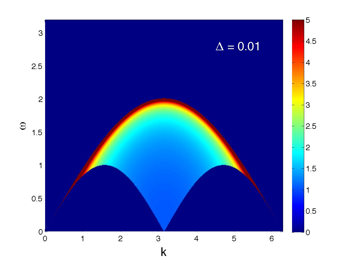
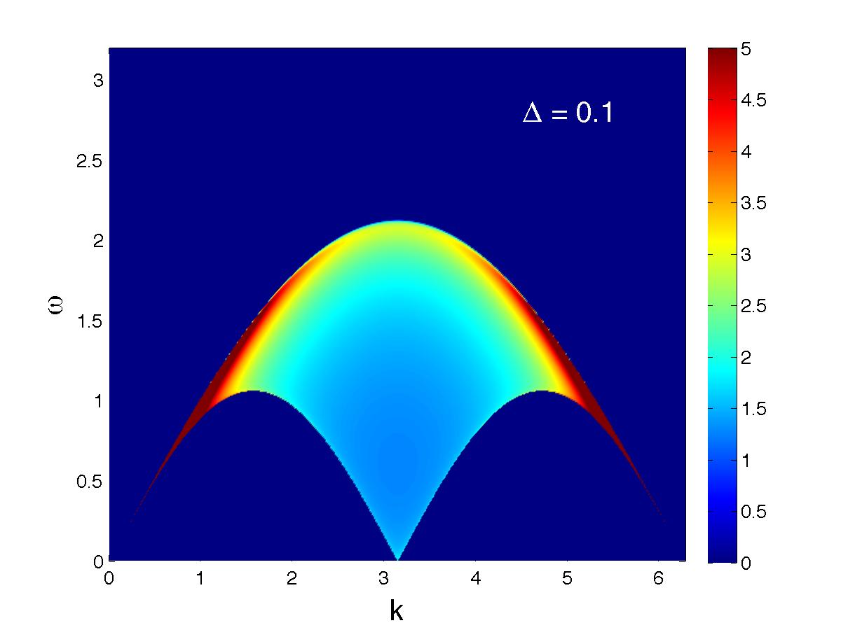
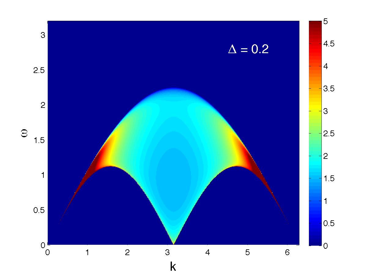
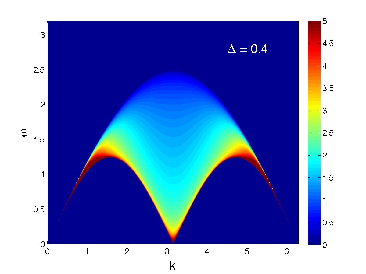
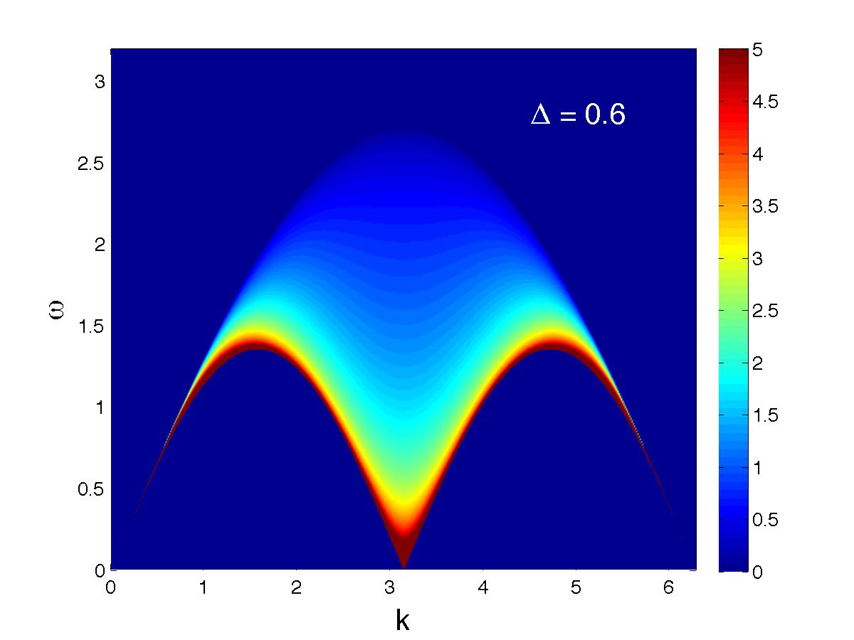
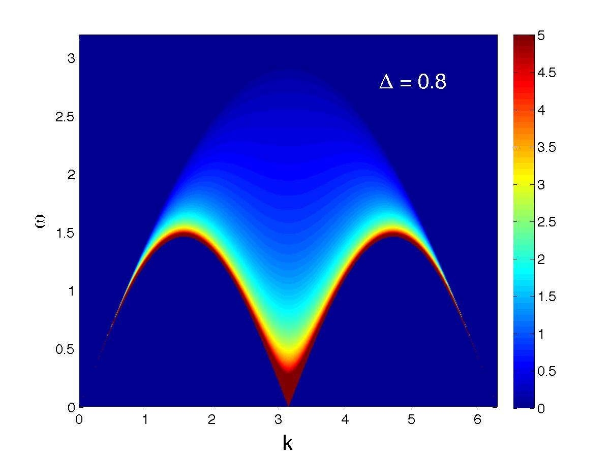
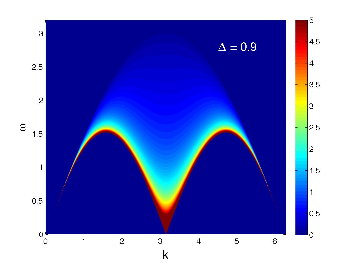
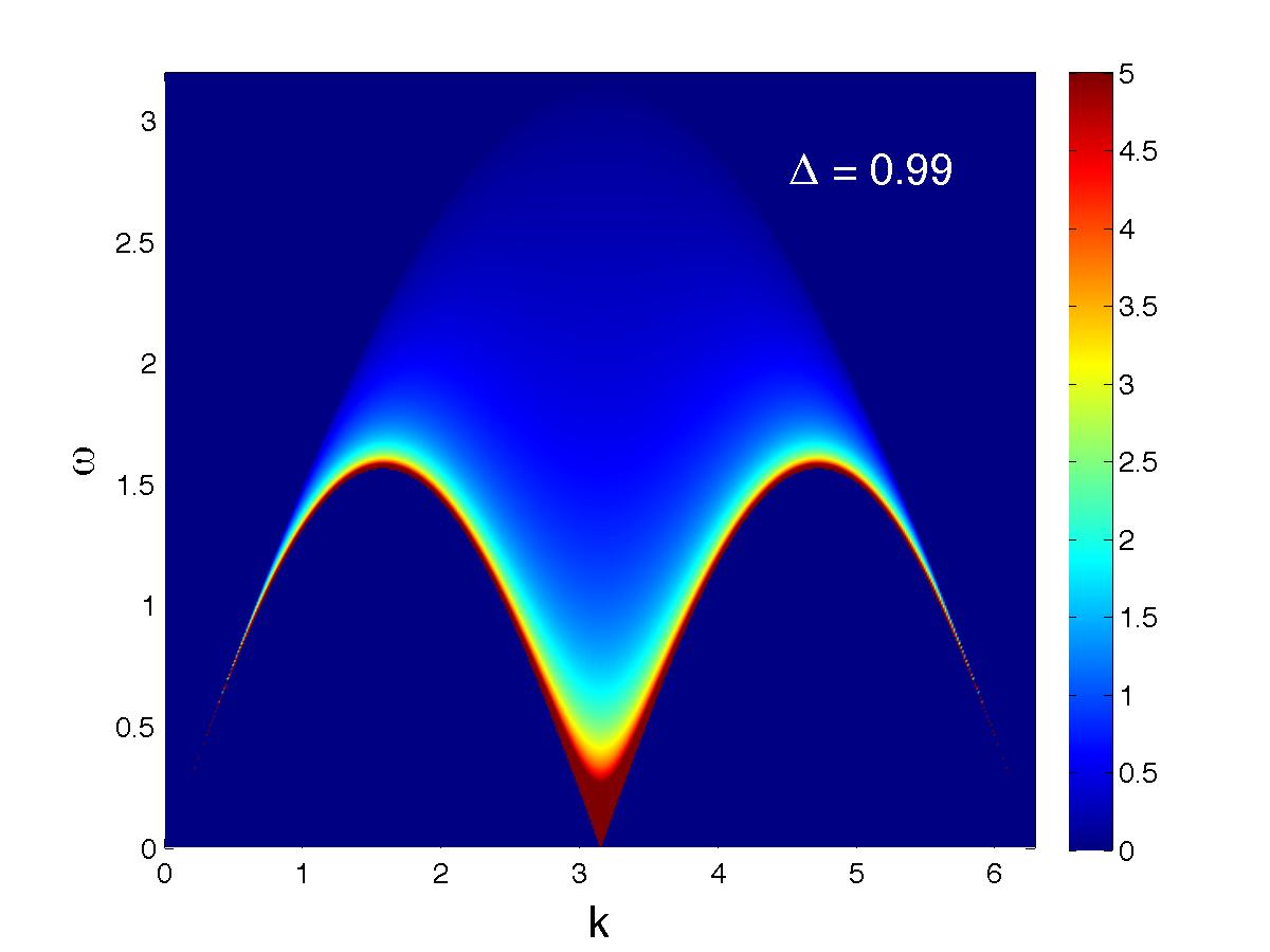
Figure 1: Two-spinon part of the longitudinal structure factor of the infinite Heisenberg chain, for different values of the anisotropy parameter $\Delta$. For $\Delta\rightarrow 0$, the correlation follows the density of states, and has a square root singularity at the upper threshold for all values of momenta. Increasing the anisotropy shifts the weight progressively towards the lower boundary. The lower boundary becomes increasingly sharp as the $\Delta\rightarrow 1$ limit is approached.

Results – In Fig.1, we give plots of the two-spinon part of the longitudinal structure factor (4) for values of $\Delta$ interpolating between weak and strong coupling. A few striking things are worth mentioning concerning the influence of interactions on the two-spinon part of the correlations. Most noticeably, upper threshold divergence disappears immediately upon turning interactions on. The correlation weight also starts flowing around the edges of the continuum, mostly via the wings at $k\simeq 0,2\pi$ (see e.g. the $\Delta=0.2$ plot), and thereafter starts accumulating at the antiferromagnetic point $k=\pi$ (see the $\Delta=0.4$ plot). The lower threshold divergence starts carrying more weight from $\Delta\simeq 0.5$ onwards, and becomes increasingly sharp as one approaches the isotropic point.

Within the two-spinon continuum, so away from the thresholds, two things can be noticed. First, the weight within the bulk of this continuum quickly changes shape as $\Delta$ is turned on: from a pure $[\omega_{2,u}(k)-\omega]^{-1/2}$ form at $\Delta=0$, it becomes almost uniform in frequency for $\Delta\simeq 0.2$; it then becomes a rapidly decreasing function of frequency for higher interactions. Turning interactions on therefore leads to a remarkable collapse of correlation weight from high to low energies.

Sum rules – To quantify the importance of the two-spinon contribution to the full structure factor, we use two useful sum rules, namely the integrated intensity

$$I^{zz}=\int_{0}^{2\pi}\frac{dk}{2\pi}\int_{0}^{\infty}\frac{d\omega}{2\pi}S(k,\omega)=1/4,$$ (7)

and the f-sumrule (at fixed momentum) Hohenberg and Brinkman (1974),

$$I^{zz}_{1}(k)=\int_{0}^{2\pi}\frac{d\omega}{2\pi}\omega S(k,\omega)=-2X^{x}(1-\cos k)$$ (8)

where $X^{x}\equiv\langle S^{x}_{j}S^{x}_{j+1}\rangle$ is the ground state expectation value of the in-plane exchange term. This can be obtained from the ground-state energy density $e_{0}$ Yang and Yang (1966) and its derivative, namely $X^{x}=\frac{1}{2J}(1-\Delta\frac{\partial}{\partial\Delta})e_{0}$, with

$$e_{0}=\frac{-J(\xi+1)}{2\pi}\sin\left[\frac{\pi}{\xi\!+\!1}\right]\int_{-\infty}^{\infty}\!\!\!dt\left(1-\frac{\tanh t}{\tanh[(\xi+1)t]}\right).$$ (9)

We provide the explicit values of the sum rule saturations coming from two-spinon contributions in Table 1 (for the f-sumrule, the saturation is the same at all momenta). The two-spinon states carry the totality of the correlation at $\Delta=0$, and this remains approximately true up to surprisingly large values of interactions $\Delta\sim 0.8$, above which four, six, … spinon states become noticeable.

$\Delta$	$I^{zz}_{2sp}/I^{zz}$	$I^{zz}_{1,2sp}/I^{zz}_{1}$		$\Delta$	$I^{zz}_{2sp}/I^{zz}$	$I^{zz}_{1,2sp}/I^{zz}_{1}$
0	1	1		0.6	0.9778	0.9743
0.1	0.9997	0.9997		0.7	0.9637	0.9578
0.2	0.9986	9.9984		0.8	0.9406	0.9314
0.3	0.9964	9.9959		0.9	0.8980	0.8844
0.4	0.9927	0.9917		0.99	0.7918	0.7748
0.5	0.9869	0.9849		0.999	0.7494	0.7331

Table 1: Sum rule saturations as a function of anisotropy: two-spinon contribution to the integrated intensity $I^{zz}$ (7) and first frequency moment $I^{zz}_{1}$ (8).

Threshold behaviour – The behaviour of the longitudinal structure factor in the vicinity of the excitation thresholds can be determined from the analytic expressions we have obtained, allowing us to make contact with and complement recent field theory predictions Pereira et al. (2008); Cheianov and Pustilnik (2008).

The structure factor near the upper threshold.

The upper threshold $\omega\rightarrow\omega_{2,u}(k)$ is approached by the limit $\rho\rightarrow 0$ as can be seen from (6). A careful evaluation shows that the integral (5) then behaves according to $I_{\xi}(\rho)~{}\begin{subarray}{c}\vspace{1mm}\\ \xrightarrow{\hskip 22.76219pt}\\ {\rho\rightarrow 0}\end{subarray}~{}-2\ln\rho+\mbox{O}(1).$ We thus have from (6) that the structure factor vanishes as a square root,

$$S^{zz}_{2}(k,\omega)~{}\begin{subarray}{c}\vspace{1mm}\\ \xrightarrow{\hskip 39.83385pt}\\ {\omega\rightarrow\omega_{2,u}(k)}\end{subarray}~{}=f_{u}(\xi)(\sin\frac{k}{2})^{-7/2}\sqrt{\omega_{2,u}(k)-\omega}$$ (10)

in which $f_{u}(\xi)$ is a momentum-independent function of anisotropy. The anisotropy-independent square-root cusp at the threshold (for $0<\Delta\leq 1$) confirms the field theory predictions Pereira et al. (2008), and at $\Delta\rightarrow 1$ matches the same limit known to apply for the $XXX$ case Karbach et al. (1997). The prefactor we obtain here varies quickly with momentum, showing strong enhancement of the upper threshold singularity when taking the momentum towards the $k=0,2\pi$ zone boundaries (as can be seen in Fig.1, most clearly at small anisotropies). For the $\Delta\rightarrow 0$ limit (so $\xi\rightarrow 1$), the $\cosh\frac{2\pi\rho}{\xi}+\cos\frac{\pi}{\xi}$ in the denominator of (4) vanishes when $\rho\rightarrow 0$. Overall, in this case one rather obtains a square-root divergence, $S^{zz}_{2}(k,\omega)~{}\begin{subarray}{c}\vspace{1mm}\\ \xrightarrow{\hskip 39.83385pt}\\ {\omega\rightarrow\omega_{2,u}(k)}\end{subarray}~{}f_{u}(1)\frac{(\sin\frac{k}{2})^{-1/2}}{\sqrt{\omega_{2,u}(k)-\omega}},$ which follows the singularity of the density of states (the matrix elements are then energy independent). This discontinuous in $\Delta$ threshold exponent behaviour is also consistent with field theory Pereira et al. (2008). We notice further that the momentum dependence of the prefactor is changed to a much weaker one than that at $\Delta\neq 0$.

The structure factor near the lower threshold.

The limit $\omega\rightarrow\omega_{2,l}(k)$ is obtained via $\rho\rightarrow\infty$. Evaluating (5) yields $I_{\xi}(\rho)~{}\begin{subarray}{c}\vspace{1mm}\\ \xrightarrow{\hskip 28.45274pt}\\ {\rho\rightarrow\infty}\end{subarray}~{}-\pi\left(1+\frac{1}{\xi}\right)\rho+\mbox{O}(1).$ The structure factor then obeys

$$S^{zz}_{2}(k,\omega)~{}\begin{subarray}{c}\vspace{1mm}\\ \xrightarrow{\hskip 39.83385pt}\\ {\omega\rightarrow\omega_{2,l}(k)}\end{subarray}=f_{l}(\xi)\frac{|\sin k|^{-\frac{1}{2}(1-\frac{1}{\xi})}(\sin\frac{k}{2})^{-\frac{2}{\xi}}}{[\omega-\omega_{2,l}(k)]^{\frac{1}{2}(1-\frac{1}{\xi})}},$$ (11)

where $f_{l}(\xi)$ is again a momentum-independent function of anisotropy. The singularity exponent reproduces an early conjecture Müller et al. (1981, 1981) and field theory predictions Pereira et al. (2008); Cheianov and Pustilnik (2008); the momentum-dependent part of the prefactor shows an even more complicated behaviour than that of the upper threshold, being enhanced (though differently) both at the zone boundaries $k=0,2\pi$ as well as near $k=\pi$. As a final detail, the $\Delta\rightarrow 0$ limit (so $\xi\rightarrow 1$) yields the expected behaviour, $S^{zz}_{2}(k,\omega)~{}\begin{subarray}{c}\vspace{1mm}\\ \xrightarrow{\hskip 39.83385pt}\\ {\omega\rightarrow\omega_{2,l}(k)}\end{subarray}~{}O(1)$.

Conclusions – In this paper, we have tracked how the spinon excitations in Heisenberg antiferromagnets contribute to the longitudinal spin structure factor (2), as a function of anisotropy (i.e. interaction). We have obtained the two-spinon part of this correlator exactly in the zero-field, infinite-size chain throughout the gapless antiferromagnetic regime, by exploiting the vertex operator approach to express states and correlators in a purely algebraic language. Our results provide an exact lower bound for and an extremely accurate description of the full correlator (as shown by sum rule saturations) throughout the observable excitation continuum (i.e. not only at low energies or near thresholds), provide a resilient check for alternate methods and give a nonperturbative derivation of the threshold exponents obtained from field theory while complementing these with exact prefactors. The precise functional form we have obtained also allows us to determine the region of validity of the threshold behaviour; we will address this and further issues in future work Caux et al. (2011).

Acknowledgements – J.-S. C. acknowledges support from the FOM foundation of the Netherlands. H.K. was supported in part by Grant-in-Aid for Scientific Research (C) 22540022. M.S. acknowledges the Australian Research Council (ARC) for financial support. The authors are grateful to L. Frappat and E. Ragoucy as organizers of the RAQIS conferences, during which this work was initiated.

References

- Haldane (1981) F. D. M. Haldane, J. Phys C: Sol. St. Phys. 14, 2585 (1981).
- Giamarchi (2004) T. Giamarchi, Quantum Physics in One Dimension (Oxford University Press, 2004).
- Landau (1957) L. D. Landau, Sov. Phys. JETP 3, 920 (1957).
- Heisenberg (1928) W. Heisenberg, Z. Phys. 49, 619 (1928).
- Orbach (1958) R. Orbach, Phys. Rev. 112, 309 (1958).
- Faddeev and Takhtajan (1981) L. D. Faddeev and L. A. Takhtajan, Phys. Lett. A 85, 375 (1981).
- Müller et al. (1981) G. Müller, H. Thomas, H. Beck, and J. C. Bonner, Phys. Rev. B 24, 1429 (1981).
- Müller et al. (1981) G. Müller, H. Thomas, M. W. Puga, and H. Beck, J. Phys. C: Sol. St. Phys. 14, 3399 (1981).
- Totsuka (1998) K. Totsuka, Phys. Rev. B 57, 3454 (1998).
- Watson et al. (2001) B. C. Watson, V. N. Kotov, M. W. Meisel, D. W. Hall, G. E. Granroth, W. T. Montfrooij, S. E. Nagler, D. A. Jensen, R. Backov, M. A. Petruska, et al., Phys. Rev. Lett. 86, 5168 (2001).
- Thielemann et al. (2009) B. Thielemann, C. Rüegg, H. M. Rønnow, A. M. Läuchli, J.-S. Caux, B. Normand, D. Biner, K. W. Krämer, H.-U. Güdel, J. Stahn, et al., Phys. Rev. Lett. 102, 107204 (2009).
- Duan et al. (2003) L.-M. Duan, E. Demler, and M. D. Lukin, Phys. Rev. Lett. 91, 090402 (2003).
- Jimbo and Miwa (1995) M. Jimbo and T. Miwa, Algebraic Analysis of Solvable Lattice Models (American Mathematical Society, Providence, RI, 1995).
- Caux and Maillet (2005) J.-S. Caux and J. M. Maillet, Phys. Rev. Lett. 95, 077201 (2005).
- Caux et al. (2005) J.-S. Caux, R. Hagemans, and J. M. Maillet, J. Stat. Mech.: Th. Exp. 2005, P09003 (2005).
- White and Feiguin (2004) S. R. White and A. E. Feiguin, Phys. Rev. Lett. 93, 076401 (2004).
- Sirker (2006) J. Sirker, Phys. Rev. B 73, 224424 (2006).
- Syljuåsen (2008) O. F. Syljuåsen, Phys. Rev. B 78, 174429 (2008).
- Pustilnik et al. (2006) M. Pustilnik, M. Khodas, A. Kamenev, and L. I. Glazman, Physical Review Letters 96, 196405 (pages 4) (2006).
- Pereira et al. (2006) R. G. Pereira, J. Sirker, J.-S. Caux, R. Hagemans, J. M. Maillet, S. R. White, and I. Affleck, Phys. Rev. Lett. 96, 257202 (2006).
- Pereira et al. (2008) R. G. Pereira, S. R. White, and I. Affleck, Phys. Rev. Lett. 100, 027206 (pages 4) (2008).
- Cheianov and Pustilnik (2008) V. V. Cheianov and M. Pustilnik, Phys. Rev. Lett. 100, 126403 (2008).
- Pereira et al. (2009) R. G. Pereira, S. R. White, and I. Affleck, Phys. Rev. B 79, 165113 (2009).
- Bougourzi et al. (1996) A. H. Bougourzi, M. Couture, and M. Kacir, Phys. Rev. B 54, R12669 (1996).
- Karbach et al. (1997) M. Karbach, G. Müller, A. H. Bougourzi, A. Fledderjohann, and K.-H. Mütter, Phys. Rev. B 55, 12510 (1997).
- Abada et al. (1997) A. Abada, A. H. Bougourzi, and B. Si-Lakhal, Nucl. Phys. B 497, 733 (1997).
- Caux and Hagemans (2006) J.-S. Caux and R. Hagemans, J. Stat. Mech: Th. Exp. p. P12013 (2006).
- Bougourzi et al. (1998) A. H. Bougourzi, M. Karbach, and G. Müller, Phys. Rev. B 57, 11429 (1998).
- Caux et al. (2008) J.-S. Caux, J. Mossel, and I. P. Castillo, J. Stat. Mech.: Th. Exp. 2008, P08006 (2008).
- Jimbo and Miwa (1996) M. Jimbo and T. Miwa, J. Phys. A: Math. Gen. 29, 2923 (1996).
- Jimbo et al. (1997) M. Jimbo, H. Konno, and T. Miwa, in Deformation theory and symplectic geometry, edited by D. Sternheimer, J. Rawnsley and S. Gutt (1997), no. 20 in Math. Phys. Studies, pp. 117 – 138, proceedings of the Ascona Meeting, June 1996.
- Baxter (1982) R. Baxter, Exactly Solved Models in Statistical Mechanics (Academic Press, 1982).
- Lashkevich and Pugai (1998a) M. Lashkevich and Y. Pugai, Nucl. Phys. B 516, 623 (1998a).
- Lashkevich and Pugai (1998b) M. Lashkevich and Y. Pugai, JETP Letters 68, 257 (1998b).
- Lashkevich (2002) M. Lashkevich, Nucl. Phys. B 621, 587 (2002).
- Kojima et al. (2005) T. Kojima, H. Konno, and R. Weston, Nucl. Phys. B 720, 348 (2005).
- Lukyanov and Terras (2003) S. Lukyanov and V. Terras, Nucl. Phys. B 654, 323 (2003).
- Caux et al. (2011) J.-S. Caux, H. Konno, M. Sorrell, and R. Weston (2011), to be published.
- Hohenberg and Brinkman (1974) P. C. Hohenberg and W. F. Brinkman, Phys. Rev. B 10, 128 (1974).
- Yang and Yang (1966) C. N. Yang and C. P. Yang, Phys. Rev. 150, 327 (1966).