Magnetic dynamics driven by the spin-current generated via spin-Seebeck effect

Abstract

We consider the spin-current driven dynamics of a magnetic nanostructure in a conductive magnetic wire under a heat gradient in an open circuit, spin Seebeck effect geometry. It is shown that the spin-current scattering results in a spin-current torque acting on the nanostructure and leading to precession and displacement. The scattering leads also to a redistribution of the spin electrochemical potential along the wire resulting in a break of the polarity-reversal symmetry of the inverse spin Hall effect voltage with respect to the heat gradient inversion.

Introduction.- The discovery in the 1820s by T.J. Seebeck that due to a temperature gradient an electric voltage emerges along the temperature drop, revealed the relationship between heat and charge currents. The reversal of Seebeck’s effect, i.e. the appearance of a temperature gradient upon an applied voltage, was shortly thereafter confirmed by J.-C. Peltier in 1834. In addition to other thermo-electric phenomena such as the Joule heating, in magnetic fields new thermo-magnetic effects arise: A resistive conductor with a temperature gradient $\mbox{\boldmath$\mathrm{\nabla}$}T$ placed in a magnetic field $\mathbf{B}$ perpedicular to $\mbox{\boldmath$\mathrm{\nabla}$}T$ develops a potential drop normal to both $\mbox{\boldmath$\mathrm{\nabla}$}T$ and $\mathbf{B}$. This phenomenon is termed the Ettingshausen effect and its reverse is the Nernst effect. In a magnetic material the anomalous Nernst effect occurs (i.e. the Nernst effect due to the spontaneous magnetization) which was first observed for Ni and Ni-Cu alloy 1 ; 2 . Recently, in Refs.3 ; 4 ; 5 ; 6 measurements of the planar and the anomalous Nernst effect were reported for a variety of materials including magnetic semiconductor, ferromagnetic metals, pure transition metals, oxides, and chalcogenides. A qualitatively new phenomena, the Spin-Seebeck effect (SSE), was discovered 2008 by Uchida et al. 7 showing that in a ferromagnetic material (a mm-size Ni₈₁Fe₁₉ sample) and in an open-circuit geometry (which is also the geometry studied in this work, cf. Fig. 1) a heat current results in a spin current, i.e. a flow of spin angular momentum and hence a spin voltage, even if $\mbox{\boldmath$\mathrm{\nabla}$}T$ is parallel to $\mathbf{B}$ (where the Nernst-Ettingshausen effect does not contribute). The spin voltage is reflected by a charge voltage that emerges (due the inverse spin Hall effect (ISHE)) in a Pt strip deposited on the sample perpendicular to $\mbox{\boldmath$\mathrm{\nabla}$}T$ (cf. Fig.1). Further experiments on resistive conductors (8 for Ni₈₁Fe₁₉), insulating ferrimagnets (LaY₂Fe₅O₁₂ in 9 ), and for ferromagnetic semiconductors (GaMnAs 10 ) underline the generality of SSE. These fascinating effects are not only of fundamental importance; thermo-electric elements are already indispensable for temperature sensing and control and for current-heat conversion. SSE opens the way for thermo-electric spintronic devices with qualitatively new tools for energy-consumption reduction. It is highly desirable to explore whether SSE can be utilized to steer localized magnetic textures, as problem addressed here. Theoretically, the reciprocity between the dynamics in the magnetic order and the heat gradients is governed by the Onsager relations. The Onsager matrix were discussed from a general point of view in Ref. 12 with a focus on the transport of charge, magnetization, and heat.

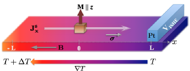
Figure 1: A localized magnetic structure $\mathrm{M}$ in a ferromagnetic conductor of length $2L$ subject to the constant temperature gradient $\mbox{\boldmath$\mathrm{\nabla}$}T$. $\mathrm{B}$ is a saturation magnetic field along $\mbox{\boldmath$\mathrm{\nabla}$}T$. The pure spin current $\mbox{\boldmath$\mathrm{J}$}^{s}_{x}$ is signaled by the inverse spin Hall voltage $V_{\mbox{ISHE}}$ measured in a Pt strip. $x$ and $z$ axes are indicted.

In Refs.13 ; 14 a thermo-magnetic mesoscopic circuit theory was put forward. Ref. 15 pointed out the occurrence of a thermally excited spin current in resistive conductors with an embedded ferromagnetic nanoclusters. Other recent works 13 ; 14 addressed the thermally induced spin-transfer torque in a spin valves structures whereas the phenomenological study 16 is focused on the spin-transfer torques in quasi one-dimensional magnetic domain walls (DWs) by introducing a viscous term into the Landau-Lifshitz-Gilbert equation (LLG).
Spin current- The microscopic mechanism for the appearance of the spin current in SSE is not yet completely understood, it is however an experimental fact that in the geometry of Fig.1 the thermal gradient $\mbox{\boldmath$\mathrm{\nabla}$}T$ generates a steady state spin current $\mbox{\boldmath$\mathrm{J}$}^{s}_{T}$ without a charge current 7 ; 8 ; 9 ; 10 . The amplitude of $\mbox{\boldmath$\mathrm{J}$}^{s}_{T}$ is found to be determined by 7 ; 8 ; 9 ; 10

$$\mbox{\boldmath$\mathrm{J}$}^{s}_{T}=-\kappa\mbox{\boldmath$\mathrm{\nabla}$}T$$ (1)

where $\kappa$ is a temperature-independent transport coefficient whose properties are discussed in 7 ; 8 ; 9 ; 10 ; no charge current is generated. The purpose of this work is to inspect the dynamics triggered by $\mbox{\boldmath$\mathrm{J}$}^{s}_{T}$ (eq.(1)) for the case where localized magnetic texture $\mathrm{M}$ note-1 is present in the ferromagnetic (FM) conductor (cf. Fig.1), a problem of great importance and has not been addressed so far. As show below, the quantum-mechanical scattering of $\mbox{\boldmath$\mathrm{J}$}^{s}_{T}$ from $\mathrm{M}$ acts in effect with a spin-current torque on $\mathrm{M}$ which results in an oscillatory and a displacement motion of $\mathrm{M}$. Upon scattering $\mbox{\boldmath$\mathrm{J}$}^{s}_{T}$ also changes. This leads to a redistribution of the spin electrochemical potential which can be measured via ISHE.

The system under consideration is illustrated in Fig. 1. Two thermal reservoirs with different temperatures $T$ and $T+\Delta T$ create along the $x$ axis in a FM conductive wire of length $2L$ a steady $T$-gradient $\mbox{\boldmath$\mathrm{\nabla}$}T$ and hence a steady-state spin current $\mbox{\boldmath$\mathrm{J}$}^{s}_{x}$. This means, without knowing the detail of the operators associated with SSE, these project the system onto a chargeless eigenstate $\psi(x)$ of the spin current operator $\mbox{\boldmath$\mathrm{j}$}_{\mu}^{s}(k)$. Generally, such a state can be written as note-2

$$\psi(x)=\frac{1}{2}\left[e^{ikx}\binom{e^{i\phi}}{e^{-i\phi}}+e^{-ikx}\binom{e^{i\theta}}{e^{-i\theta}}\right].$$ (2)

The $x$ expectation value of the charge current $\mbox{\boldmath$\mathrm{j}$}^{e}(k)=\frac{i\hbar}{2m}[(\mbox{\boldmath$\mathrm{\nabla}$}\psi^{{\dagger}}(x))\psi(x)-\psi^{{\dagger}}(x)\mbox{\boldmath$\mathrm{\nabla}$}\psi(x)]$ vanishes, i.e. $j^{e}_{x}(k)\equiv 0$ (here $m$ is the effective mass). In contrast, for the spin current $\mbox{\boldmath$\mathrm{j}$}_{\mu}^{s}(k)=\frac{i\hbar}{2m}[(\mbox{\boldmath$\mathrm{\nabla}$}\psi^{{\dagger}}(x))\sigma_{\mu}\psi(x)-\psi^{{\dagger}}(x)\sigma_{\mu}\mbox{\boldmath$\mathrm{\nabla}$}\psi(x)]$ we infer

$$j^{s}_{x}(k)=\frac{\hbar k}{2m}(\cos 2\phi-\cos 2\theta),$$ (3)

$$j^{s}_{y}(k)=\frac{\hbar k}{2m}(\sin 2\theta-\sin 2\phi).$$ (4)

In general, the thermal transport is ballistic T-transport but with diffusive spins, i.e., upon creating (2) the spin coherence is lifted by scattering events that randomize $\phi$ and $\theta$ within $[0,2\pi]$. Hence, the expectation value of the spin current vanishes on the scale of the spin-flip diffusion length semicl-theory ; spin-pumping , i.e., $\mbox{\boldmath$\mathrm{J}$}^{s}_{\mu}(k)=\oint\mbox{\boldmath$\mathrm{j}$}^{s}_{\mu}d\theta d\phi/(2\pi)^{2}=0$. However, when the wire is magnetically polarized and driven to saturation by the magnetic field $\mathrm{B}$ 7 ; 8 ; 9 ; 10 , we find $\langle\sigma_{x}\rangle\neq 0$ but $\langle\sigma_{y}\rangle=0$. Eq.(2) reads then for an exchange-split conductor

$$\psi_{B}(x)=\frac{1}{2}\left[e^{ikx}\binom{1}{1}+e^{-ikx}\binom{e^{i\theta}}{e^{-i\theta}}\right].$$ (5)

Here $\theta\in[0,2\pi]$ still appears due to the residual spin precession and diffusion. Then we have $J^{e}\equiv 0$, $J^{s}_{y}(k)=\oint j^{s}_{y}d\theta/2\pi=0$, whereas $J^{s}_{x}(k)=J^{s}_{0}(k)=\hbar k/2m$ in line with the experimental observation 7 ; 8 ; 9 ; 10 .

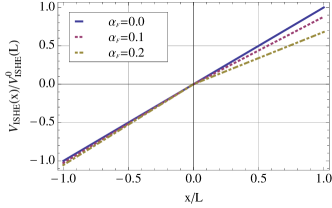
Figure 2: The electric voltage $\text{V}_{\text{ISHE}}$ generated by the inverse spin-Hall effect in the Pt layer as a function of the magnetic scattering strength $\alpha_{F}=gM_{0}m/k_{F}\hbar^{2}$ with $k_{F}$ being the Fermi wave vector. The relaxation rate is $\Gamma/E_{F}=0.01$.

The main purpose of the present work is to investigate the influence of a localized magnetic, non-diffusive scatterer $\mathrm{M}$ (where $x=0$ is taken as its central position (see Fig.1)). $\mathrm{M}$ has a uniaxial anisotropy along an axis chosen to be $z$. If $\mbox{\boldmath$\mathrm{M}$}(x)$ has an internal structure, e.g. a non-collinearity, which varies on a scale larger than $\lambda=2\pi/k$ (the variation scale of (5)), one can unitary transform to align locally with $\mathrm{M}$ which introduces a weak gauge potential that can be dealt tobepub with in a perturbative way using the Green’s function constructed from (5) (similarly as done in nick ; jpa ). We find $\mathrm{M}$ has a stronger influence if its range of variation is comparable to $\lambda$. In this case the magnetic texture acts in effect as $\mbox{\boldmath$\mathrm{M}$}(x)=\mbox{\boldmath$\mathrm{M}$}_{0}\delta(x)$, where the magnetic moment $\mbox{\boldmath$\mathrm{M}$}_{0}$ derives from an average of $\mbox{\boldmath$\mathrm{M}$}(x)$ over its extension $w$. The model is realizable for 10 rather then for metals. The interaction between $\mathrm{M}$ and the electron spin $\mathrm{\sigma}$ reads M-nanowire ,

$$H_{int}=g\mbox{\boldmath$\mathrm{M}$}(x)\cdot\mbox{\boldmath$\mathrm{\sigma}$}$$ (6)

where $g$ is a local coupling constant and $M_{0}$ is large enough to be treated classically. For $\mbox{\boldmath$\mathrm{M}$}_{0}$ aligned with $z$ axis, as in Fig.1, we derive using eqs.(5,6) the expression for the spinor wave function in the presence of $\mbox{\boldmath$\mathrm{M}$}(x)$, namely

$$\psi_{s}(x)=\begin{cases}\frac{e^{ikx}}{2}\binom{1}{1}+\frac{e^{-ikx}}{2}\binom{r}{r^{\star}}+\frac{e^{-ikx}}{2}\binom{te^{i\theta}}{t^{\star}e^{-i\theta}}&\text{for }x<0,\\ \frac{e^{-ikx}}{2}\binom{e^{i\theta}}{e^{-i\theta}}+\frac{e^{ikx}}{2}\binom{re^{i\theta}}{r^{\star}e^{-i\theta}}+\frac{e^{ikx}}{2}\binom{t}{t^{\star}}&\text{for }x>0.\end{cases}$$ (7)

The scattering state $\psi_{s}(x)$ describes the spinor wave function in the original spin channel, which is partially reflected into the original-spin and the spin-flip channels, and also partially transmitted into theses two channel, which gives the complex spin reflection and transmission coefficients $r$ and $t$,

$$r=-\frac{i\alpha}{1+i\alpha},\;t=\frac{1}{1+i\alpha},\quad\alpha=gM_{0}m/k\hbar^{2}.$$ (8)

The magnetic scattering gives rise to a short pseudo-circuit to the charge channels, for we find

$$j^{e}_{x}=\frac{2\alpha\sin\theta}{1+\alpha^{2}}.$$ (9)

$\langle j^{e}_{x}\rangle$ vanishes however beyond the spin diffusion length after averaging over $\theta$. Counterparts, i.e. a pure spin current generated by a charge current when scattered off a magnetic structure, are well known, e.g. M-nanowire ; MTJ ; miguel . The spin current carried by (5) is modified upon scattering and a none-zero $J^{s}_{y}$ emerges

$$J_{x}^{s}/J^{s}_{0}=\begin{cases}\frac{1+3\alpha^{2}}{(1+\alpha^{2})^{2}}&\text{for }x<0,\\ \frac{1-\alpha^{2}}{(1+\alpha^{2})^{2}}&\text{for }x>0,\end{cases}$$ (10)

$$J_{y}^{s}/J^{s}_{0}=\begin{cases}\frac{2\alpha^{3}}{(1+\alpha^{2})^{2}}&\text{for }x<0,\\ \frac{2\alpha}{(1+\alpha^{2})^{2}}&\text{for }x<0.\end{cases}$$ (11)

Within linear response, the spin voltage along the wire is $\mu_{s}(x)=\xi_{s}x\langle J^{s}_{x}(\alpha)\rangle$ where $\xi_{s}$ is a function of the elementary charge, the spin-dependent electric conductivity, the spin-dependent Seebeck coefficient, and the spin-Seebeck coefficient of the FM wire phe-theory . The quantum-mechanically averaged spin current is $\langle J^{s}_{x}(\alpha)\rangle=Tr(J^{s}_{x}(\alpha)\rho)$ dbbprb . The single electron density matrix is $\rho=-\frac{1}{\pi}\text{Im}\sum_{\mbox{\boldmath$\mathrm{k}$}}\frac{\psi_{s}\psi_{s}^{{\dagger}}}{E_{F}-E_{\mbox{\boldmath$\mathrm{k}$}}+i\Gamma}$ where $E_{F}$ is the Fermi energy, $E_{\mbox{\boldmath$\mathrm{k}$}}=\hbar^{2}k^{2}/2m+\hbar^{2}\mbox{\boldmath$\mathrm{k}$}_{\|}^{2}/2m$ with $\mbox{\boldmath$\mathrm{k}$}_{\|}$ being the transverse wave vector, and $\Gamma$ is a Lorenzian relaxation rate due to disorder LorenzianWidth . Depositing a conductive strip with a strong spin-orbit coupling, e.g. Pt, as shown in Fig.1, $\mu_{s}(x)$ can be imaged via the electric voltage $V_{\text{ISHE}}$ generated by the inverse spin-Hall effect in Pt using the relation

$$\frac{\text{V}_{\text{ISHE}}(x)}{\text{V}^{0}_{\text{ISHE}}(L)}=\frac{\langle J^{s}_{x}(\alpha)\rangle}{\langle J^{s}_{x}(0)\rangle}\frac{x}{L}$$ (12)

where $\text{V}^{0}_{\text{ISHE}}(x)$ is the electric voltage measured in Pt in absence of the magnetic scatterer $\mathrm{M}$. Explicitly, $\text{V}^{0}_{\text{ISHE}}(x)=\gamma\xi_{s}x\langle J^{s}_{x}(0)\rangle$ with $\gamma$ being a system-dependent parameter 7 ; 8 ; 9 ; 10 , determined by the spin-Hall angle in Pt, the spin-injection efficiency across the FM/Pt interface, and the length and the thickness of Pt wire. Due to the spin current scattering off $\mathrm{M}$ the Hall voltage $\text{V}_{\text{ISHE}}$ losses its odd symmetry with respect to a reflection at $x=0$, i.e. we deduce $-\text{V}_{\text{ISHE}}(-x)\neq\text{V}_{\text{ISHE}}(x)$. As shown in Fig.2 the amount of the symmetry break depends on $\alpha$, and can be taken in the experiment as an indicator of the presence of magnetic scattering centers.

Magnetization dynamics.- In as much as $J^{s}_{x}$ is modified by the presence of $\mathrm{M}$, the scattering triggers a dynamics of $\mathrm{M}$ which is usually much slower than the carrier scattering dynamics and can be classically treated ($M_{0}$ is assumed large). $J^{s}_{x}$ acts on $\mathrm{M}$ with a torque $T_{\mu}$ that follows from the jump in the spin current at the point $x=0$, $T_{\mu}=J^{s}_{\mu}(0^{-})-J^{s}_{\mu}(0^{+})$. Hence, $T_{\mu}$ derives from our quantum mechanical calculations as

$$T_{x}=J^{s}_{0}\frac{4\alpha^{2}}{(1+\alpha^{2})^{2}},\;T_{y}=-J^{s}_{0}\frac{2\alpha(1-\alpha^{2})}{(1+\alpha^{2})^{2}}.$$ (13)

Both components are transversal. $T_{y}$ tends to align $\mathrm{M}$ to the direction of the FM magnetization, while $T_{x}$ tries to rotate the moment $\mathrm{M}$ around the axis $\hat{e}_{x}$. Equivalently, within our model, the spin-current torque $T_{\mu}$ is obtained from the spin density $S_{\mu}(x)$ accumulated at the localized moment (due to interference of incoming and reflected waves) as

$$T_{\mu}=-\frac{gM_{0}}{\hbar}[\mbox{\boldmath$\mathrm{n}$}\times\mbox{\boldmath$\mathrm{S}$}(x=0)]$$ (14)

where $\mathrm{n}$ is the unit vector along $\mathrm{M}$, and the spin density we obtain from $S_{\mu}(x)=\psi^{{\dagger}}(x)\sigma_{\mu}\psi(x)$. Since $M_{0}$ is assumed large (say $\geq 5/2\;\mu_{B}$) the spin current-induced magnetization dynamics can be treated with the modified LLG equation emLLG ; smLLG

$$\frac{\partial\mbox{\boldmath$\mathrm{n}$}}{\partial t}=\frac{D_{z}}{\hbar}[\mbox{\boldmath$\mathrm{n}$}\times\hat{e}_{z}]+\frac{a_{g}}{\hbar}\mbox{\boldmath$\mathrm{n}$}\times\frac{\partial\mbox{\boldmath$\mathrm{n}$}}{\partial t}-\frac{g}{\hbar}[\mbox{\boldmath$\mathrm{n}$}\times\mbox{\boldmath$\mathrm{S}$}(0)]$$ (15)

where $D_{z}$ is the anisotropy energy and $a_{g}$ is the Gilbert damping parameter footn2 . Two motion types of $\mathrm{M}$ occur:

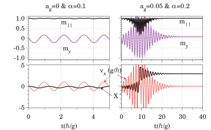
Figure 3: Precession of the magnetic moment $\mathrm{M}$ (eq.(16)) for different spin-current scattering strength $\alpha$ (cf. eq.8) and Gilbert damping $a_{g}$. Here $v_{x}=\partial X/\partial t$ and $D_{z}/g=5$.

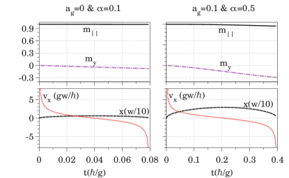
Figure 4: Displacement of the magnetic moment (given by eq.(17)) vs. time for the same parameters of Fig.3. $v_{x}=\partial x/\partial t$.

Precession- Introducing the following magnetization distribution

$$\mbox{\boldmath$\mathrm{n}$}=[m_{\|}(t)\sin X(t),m_{y}(t),m_{\|}(t)\cos X(t)]$$ (16)

and propagating with the LLG equation (Eq.15) starting from $m_{\|}(0)=1,\;m_{y}(0)=0,\;\text{and }X(0)=0$, we calculate the time dependence of $\mathrm{M}$ shown in Fig.3. The oscillations of $X(t)$ results in small $x$ and $y$ components of the magnetization. The magnetic moment precesses with a velocity $v_{x}(t)=\partial X(t)/\partial t$ in the presence of the SSE-generated spin current ($v_{x}(0)\neq 0$). We note that the maximum deflection angle $X_{max}$ depends implicitly on the spin current dynamics through the parameter $\alpha$, as determined by eq. (8). Also the Fermi energy enters through the $k$ dependence of $\alpha$. The dynamics is a mixture of anisotropy-dominated precession and damping.

Displacement- Let us consider the initial localized magnetic moment distribution

$$\mathrm{n} = [m_{\|}(t)\sin\zeta,m_{y}(t),m_{\|}(t)\cos\zeta]$$

$$\zeta = \cos^{-1}\left[\tanh^{2}(x/w)\right]$$ (17)

where $w$ stands for the extension of the localized moment and $m_{\|}(0)=1,\;m_{y}(0)=0,\;x(0)=0.$ As concluded from Fig.4, the moment is set in motion when subjected to the spin current. The velocity changes from positive to negative, which is different from the motion of a single Néel wall DWs (the velocity decreases to zero in a fraction of a nanosecond, and the DWs stops completely.).

Remarks and conclusions.- Our main result is that the SSE generated spin current in a wire may scatter from a localized magnetic structure setting it in an precessional and a displacement motion. The scattering also leads to a redistribution of the spin current in the wire and hence changes the ISHE signal. From these results conclusion can be made on the influence of a collection of non-interacting localized moments but no statement can be made when they interact or even form clusters. We also note that the present conclusions do not apply to a domain wall (DW), (except for very close non-resonant (transversal) $180^{\circ}$ DW pair, e.g. as in vitaprl ). In fact, our initial finding tobepub is that a single sharp DW is less affected by the spin current because the spin-current torques acting from left and right of the DW partially compensate. This is not so for an adiabatic or asymmetric DW because the $T$-gradient modifies the DW along $\mbox{\boldmath$\mathrm{\nabla}$}T$. As for the experimental observation of the magnetic moment dynamics, it should be noted that the temperature gradient has to be sustained on the time-scale of this dynamics; a fast (e.g., femtosecond) strong heat pulse is inappropriate for our (constant $\nabla T$, linear response) study and may cause locally a longitudinal dynamics of $\mathrm{M}$.

References

- (1) V.W. Rindner and K. M. Koch, Z. Naturforsch. 13a, 26 (1958).
- (2) V. G. Nentwich, Z. Naturforsch. 19a, 1137 (1964).
- (3) Y. Onose, Y. Shiomi, Y. Tokura, Phys. Rev. Lett. 100, 016601 (2008).
- (4) Y. Pu, E. Johnston-Halperin, D.D. Awschalom, J. Shi, Phys. Rev. Lett. 97, 036601 (2006).
- (5) Y. Pu, D. Chiba, F. Matsukura, H. Ohno, J. Shi, Phys. Rev. Lett. 101, 117208 (2008).
- (6) T. Miyasato, it al., Phys. Rev. Lett. 99, 086602 (2007).
- (7) K. Uchida, it al., Nature 455, 346 (2008).
- (8) K. Uchida, it al., Solid State Commun. 150, 524 (2010).
- (9) K. Uchida, it al., Nature Mat. 9, 894 (2010).
- (10) C. M. Jaworski, it al., Nature Mat. 9, 898 (2010).
- (11) M. Johnson, R.H. Silsbee, Phys. Rev. B 35, 4959 (1987).
- (12) M. Hatami, G.E.W. Bauer, Q. Zhang, P.J. Kelly, Phys. Rev. B 79, 174426 (2009).
- (13) M. Hatami, G.E.W. Bauer, Q. Zhang, P.J. Kelly, Phys. Rev. Lett. 99, 066603 (2007).
- (14) O. Tsyplyatyev, O. Kashuba, V.I. Falko, Phys. Rev. B 74, 132403 (2006).
- (15) A.A. Kovalev, Y. Tserkovnyak, arXiv:0906.1002v2.
- (16) As an example, we take a single-molecule magnets Mn12 [Mn12O12(O2C-C6H4-SAc)16(H2 O)4] as the local magnetic scatterer . The total spin and diameter of Mn12 are and nm, respectively Mn12 . The local exchange coupling between the carriers and the moment is given as meV SMMT .
- (17) H. B. Heersche, Z. de Groot, J. A. Folk, and H.S. J. van der Zant, Phys. Rev. Lett. 96, 206801 (2006).
- (18) R.Q. Wang, L. Sheng, R. Shen, B. Wang, and D.Y. Xing, Phys. Rev. Lett. 105, 057202 (2010).
- (19) We employ a continuous model; a discretized treatment based on Heisenberg spins is straightforward and does not alter qualitatively the amplitude of the spin/charge current.
- (20) X. Zotos, F. Naef, and P. Prelovšek, Phys. Rev. B 55, 11029 (1997); A. V. Sologubenko, it al., Phys. Rev. B 62, R6108 (2000).
- (21) M. Hatami, G. E. W. Bauer, S. Takahashi, and S. Maekawa, Solid State Commun. 150, 480 (2010).
- (22) J. Xiao, G. E. W. Bauer, K.-C. Uchida, E. Saitoh, and S. Maekawa, Phys. Rev. B 81, 214418 (2010).
- (23) C.L. Jia, J. Berakdar, unpublished.
- (24) N. Sedlmayr, V. K. Dugaev, and J. Berakdar, Phys. Rev. B 79, 174422 (2009); Phys. Status Solidi B 247, 2603 (2010).
- (25) V. K. Dugaev, J. Barnas and J. Berakdar, J. Phys. A 36, 9263 (2003).
- (26) V. K. Dugaev, V. R. Vieira, P. D. Sacramento, J. Barnaś, M. A. N. Araújo, and J. Berakdar, Phys. Rev. B 74, 054403 (2006).
- (27) A. Vedyayev, M. Chschiev, and B. Dieny, J. Phys.: Condens. Matter 20, 145208 (2008); A. Manchon, N. Ryzhanova, A. Vedyayev, M. Chschiev, and B. Dieny, J. Phys.: Condens. Matter 20, 145208 (2008).
- (28) M. Araujo, V. Dugaev, V. Veira, J. Berakdar, and J. Barnas, Phys. Rev. B 74, 224429 (2006).
- (29) K. Uchida, it al., J. Appl. Phys. 105, 07C908 (2010).
- (30) V. K. Dugaev, J. Berakdar, and J. Barnaś, Phys. Rev. B 68, 104434 (2003).
- (31) O. E. Dial, R. C. Ashoori, L. N. Pfeiffer and K. W. West, Nature(London) 448, 176 (2007).
- (32) Ya. B. Bazaliy, B. A. Jones, and S.-C. Zhang, Phys. Rev. B 57, R3213 (1998).
- (33) J. Fernández-Rossier, M. Braun, A. S. Nú nez, and A. H. MacDonald, Phys. Rev. B 69, 174412 (2004).
- (34) Temperature effects can be included in eq.(15) as in alexander . by assuming to be in a local thermal equilibrium at the temperature (assuming ) an applying the fluctuation-dissipation theorem which yields a stochastic field that adds to the effective field in eq.(15). In alexander it is shown that at low thermal fluctuations do not alter qualitatively the LLG dynamics.
- (35) A. Sukhov, J. Berakdar, Phys. Rev. Lett. 102, 057204 (2009).
- (36) Z. Li and S. Zhang, Phys. Rev. Lett. 92, 207203 (2004).
- (37) V. Dugaev, J. Berakdar, and J. Barnas, Phys. Rev. Lett. 96, 047208 (2006).