Riemannian $\mathbf{(1+d)}$-Dim Space-Time Manifolds with Nonstandard Topology
which Admit Dimensional Reduction to Any Lower Dimension
and Transformation of the Klein-Gordon Equation
to the $\mathbf{1}$-Dim Schrödinger Like Equation

Abstract

This rather technical paper presents some generalization of the results of recent publications Shirkov2010 ; DVPF2010 ; PFDV2010 where toy models of dimensional reduction of space-time were considered.

Here we introduce and consider a specific type of multidimensional space-times with nontrivial topology and nontrivial Riemannian metric, which admit a reduction of the dimension $d$ of the space to any lower one $d_{low}=1,2,\dots,d-1$. The variable geometry is described by several variable radii of compactification of part of space dimensions.

We succeed once more in transforming the shape of the variable geometry of the $d$-dimensional spaces under consideration to a specific potential interaction, described by the potential $V$ in the one-dimensional Schrödinger-like equation.

This way one may hope to study the possible physical signals going from both higher and lower dimensions into our obviously four dimensional real world.

I Introduction

First, let us consider a $(1+3)$-Dim manifold $\mathbb{M}^{(1,3)}_{t\phi_{1}\phi_{2}z}$ as a hypersurface in a flat pseudo-Euclidean $(1+5)$-Dim space $\mathbb{E}^{(1,5)}_{x^{0}x^{1}x^{2}x^{3}x^{4}x^{5}}$ with signature $\{+,-,-,-,-,-,\}$ defined by the equations:

$$\mathbb{M}^{(1,3)}_{t\phi_{1}\phi_{2}z}:\left\{\begin{array}[]{cccc}x^{0}=t,\,\,\,\,x^{1}=\rho_{1}(z)\cos\phi_{1},\,\,\,\,x^{3}=\rho_{2}(z)\cos\phi_{2},\cr x^{5}=z,\,\,\,\,x^{2}=\rho_{1}(z)\sin\phi_{1},\,\,\,\,x^{4}=\rho_{2}(z)\cos\phi_{2},\end{array}\right.$$ (I.3)

assuming $t\in(-\infty,\infty)$, $z\in(-\infty,\infty)$, and $\phi_{1,2}\in[0,2\pi]$. It is obvious from (I.3) that the manifold $\mathbb{M}^{(1,3)}_{t\phi_{1}\phi_{2}z}$ has a structure $\mathbb{M}^{(1,3)}_{t\phi_{1}\phi_{2}z}=\mathbb{R}^{(1)}_{t}\otimes\mathbb{T}^{(2)}_{\phi_{1}\phi_{2}}\otimes\mathbb{R}^{(1)}_{z}$, $\mathbb{T}^{(2)}_{\phi_{1}\phi_{2}}$ being the torus $\mathbb{T}^{(2)}_{\phi_{1}\phi_{2}}=\mathbb{S}^{(1)}_{\phi_{1}}\otimes\mathbb{S}^{(1)}_{\phi_{2}}$, see Fig.1.

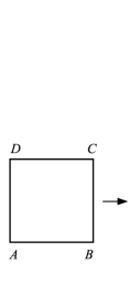
Figure 1: Obtaining torus from a square by gluing the corresponding boundaries      – a graphical representation of the double-periodic boundary conditions

Physically this means that we consider the square $\{\phi_{1},\phi_{2}\}\in[0,2\pi]\otimes[0,2\pi]$ as a flat domain with periodic boundary conditions for any field $\Psi(t,\phi_{1},\phi_{2},z)\equiv\Psi(t,\phi_{1}+2n_{1}\pi,\phi_{2}+2n_{2}\pi,z)$, $n_{1},n_{2}$ being arbitrary integers. Thus we compactify some of the space dimensions, but instead of fixing the radii of compactification $\rho_{1}(z)$ and $\rho_{2}(z)$, we let them to depend on the non-compactified coordinate $z$. In the domains of very big values of the radii $\rho_{1}(z)$ and $\rho_{2}(z)$ the space will look like the usual flat $3$-Dim space. If one or two of the radii of compactification $\rho_{1}(z)$ and $\rho_{2}(z)$ become very small, the dimension of the $3$-Dim space effectively reduces to a lower one.

The manifold (I.3) is an obvious generalization of the $(1+2)$-Dim manifolds with cylindrical symmetry, considered in Shirkov2010 ; DVPF2010 ; PFDV2010 . There we had $x^{4}$ and $x^{5}$ with fixed values, say zero.

II The Induced Riemannian Geometry of the Manifold $\mathbb{M}^{(1,3)}_{t\phi_{1}\phi_{2}z}$

The restriction of the $6$-Dim (pseudo)Euclidean interval ${}^{(6)}\!ds^{2}=(dx^{0})^{2}-(dx^{1})^{2}-(dx^{2})^{2}-(dx^{3})^{2}-(dx^{4})^{2}-(dx^{5})^{2}$ on the manifold (I.3) induces the following simple (pseudo)Riemannian $4$-Dim interval

$$ds^{2}=dt^{2}-\rho_{1}(z)^{2}d\phi_{1}^{2}-\rho_{2}(z)^{2}d\phi_{2}^{2}-\left(1+\rho_{1}^{\prime}(z)^{2}+\rho_{2}^{\prime}(z)^{2}\right)dz^{2}.$$ (II.1)

The $3$-Dim (to be physical) space with Riemannian interval

$$dl^{2}=\rho_{1}(z)^{2}d\phi_{1}^{2}+\rho_{2}(z)^{2}d\phi_{2}^{2}+\left(1+\rho_{1}^{\prime}(z)^{2}+\rho_{2}^{\prime}(z)^{2}\right)dz^{2}$$ (II.2)

has a nontrivial scalar curvature

$${}^{(3)}\!R= 2 {\frac{\big{(}\rho_{2}(z)\left((1+\rho_{2}^{\prime}(z)^{2}\right))-\rho_{1}(z)\rho_{1}^{\prime}(z)\rho_{2}^{\prime}(z)\big{)}\rho_{1}^{\prime\prime}(z)}{\rho_{1}(z)\rho_{2}(z)\big{(}1+(\rho_{1}^{\prime}(z))^{2}+(\rho_{2}^{\prime}(z))^{2}\big{)}^{2}}}+$$

$$+ 2 {\frac{\big{(}\rho_{1}(z)\left((1+\rho_{1}^{\prime}(z)^{2}\right))-\rho_{2}(z)\rho_{1}^{\prime}(z)\rho_{2}^{\prime}(z)\big{)}\rho_{2}^{\prime\prime}(z)}{\rho_{1}(z)\rho_{2}(z)\big{(}1+(\rho_{1}^{\prime}(z))^{2}+(\rho_{2}^{\prime}(z))^{2}\big{)}^{2}}}+$$

$$+ 2 {\frac{\rho_{1}^{\prime}(z)\rho_{2}^{\prime}(z)}{\rho_{1}(z)\rho_{2}(z)\big{(}1+(\rho_{1}^{\prime}(z))^{2}+(\rho_{2}^{\prime}(z))^{2}\big{)}}},$$ (II.3)

but its $3$-Dim Weyl tensor vanishes identically. Since we deal with a nontrivial $3$-Dim Riemannian manifold, the vanishing of the Weyl tensor is not sufficient to conclude that the physical space with metric (II.2) is conformally flat. The necessary and sufficient condition for conformal flatness of $3$-Dim space is to vanish its Taub tensor Taub

$${}^{(3)}T_{\alpha\beta\gamma}=\triangledown_{\alpha}\left({}^{(3)}\!R_{\beta\gamma}-(1/4){}^{(3)}\!R\,{}^{(3)}\!g_{\beta\gamma}\right)-\triangledown_{\beta}\left({}^{(3)}\!R_{\alpha\gamma}-(1/4){}^{(3)}\!R\,{}^{(3)}\!g_{\alpha\gamma}\right).$$

In general, for the metric in (II.2) the Taub tensor does not vanish. It is easy to check that the $4$-Dim pseudo-Riemannian manifold with metric (II.1) is not conformally flat, too, since its $4$-Dim Weyl tensor does not vanish.

In the space-times at hand the $4$-Dim scalar curvature coincides with the $3$-Dim one (II.3), i.e., ${}^{(4)}\!R={}^{(3)}\!R$.

The obtained $3$-Dim metric is diagonal with diagonal elements $\rho_{1}(z)^{2}$, $\rho_{2}(z)^{2}$, and $\rho_{3}(z)^{2}=1+(\rho_{1}^{\prime}(z))^{2}+(\rho_{2}^{\prime}(z))^{2}$. The square root of its determinant is $\sqrt{{}^{(3)}\!g(z)}=\rho_{1}(z)\rho_{2}(z)\rho_{3}(z)=\sqrt{{}^{(4)}\!g(z)}$.

The natural (orthogonal) tetrad basis $e^{(a)}_{\alpha}(z)$ $\big{(}g_{\alpha\beta}(z)=e^{(a)}_{\alpha}(z)e^{(b)}_{\beta}(z)\eta_{ab}\big{)}$ for the $4$-Dim interval (II.1) is needed to construct the Dirac equation, see for example the recent articles Teryaev2005 ; Teryaev2009 ; Neznamov and the references therein. In our case this basis is a very simple one:

$$e^{(0)}_{\alpha}(z)=\left(\begin{array}[]{c}1\\ 0\\ 0\\ 0\end{array}\right),\,\,\,\,e^{(1)}_{\alpha}(z)=\left(\begin{array}[]{c}0\\ \rho_{1}(z)\\ 0\\ 0\end{array}\right),\,\,\,\,e^{(2)}_{\alpha}(z)=\left(\begin{array}[]{c}0\\ 0\\ \rho_{2}(z)\\ 0\end{array}\right),\,\,\,\,e^{(3)}_{\alpha}(z)=\left(\begin{array}[]{c}0\\ 0\\ 0\\ \rho_{3}(z)\end{array}\right).$$ (II.20)

Since the $3$-Dim space is not conformally flat, the methods for studying the Dirac equation used in Teryaev2005 ; Teryaev2009 are not directly applicable to space-times with metric (II.1) if one does not consider the very special case $\rho_{1}(z)=\rho_{2}(z)=\rho_{3}(z)$.

Obviously, taking the limit $\rho_{1}(z)\to 0$, or the limit $\rho_{2}(z)\to 0$, we are able to make a reduction of dimension of the physical space from $d=3$ to $d=2$. The simultaneous limits $\rho_{1}(z)\to 0$ and $\rho_{2}(z)\to 0$ will bring us to a one-dimensional physical space ($d=1$). Hence, working with the toy-metric (II.1), we are able to study different physical phenomena, related with dimensional reduction Shirkov2010 ; DVPF2010 ; PFDV2010 exploring all physically interesting lower dimensions: $d_{low}=1,2$.

III The $3$-Dim Laplacian, new variables and reduction of the Klein-Gordon equation to the $\mathbf{1}$-Dim Schrödinger like one

In the coordinates $\phi_{1},\phi_{2},z$ the $3$-Dim Laplacian reads

$$\Delta_{3}={\frac{1}{\rho_{1}(z)^{2}}}\partial^{2}_{\phi_{1}}+{\frac{1}{\rho_{2}(z)^{2}}}\partial^{2}_{\phi_{2}}+{\frac{1}{\rho_{1}(z)^{2}\rho_{2}(z)^{2}}}\left({\frac{\rho_{1}(z)\rho_{2}(z)}{\rho_{3}(z)}}\partial_{z}\left({\frac{\rho_{1}(z)\rho_{2}(z)}{\rho_{3}(z)}}\partial_{z}\right)\right).$$ (III.1)

The introduction of the new variable

$$u=u(z)=\int{\frac{\rho_{3}(z)}{\rho_{1}(z)\rho_{2}(z)}}dz=\int{\frac{\sqrt{1+\rho_{1}^{\prime}(z)^{2}+\rho_{2}^{\prime}(z)^{2}}}{\rho_{1}(z)\rho_{2}(z)}}dz$$ (III.2)

is analogous to the one used in PFDV2010 and simplifies the form of the $3$-D Laplacian:

$$\Delta_{3}={\frac{1}{\varrho_{1}(u)^{2}}}\partial^{2}_{\phi_{1}}+{\frac{1}{\varrho_{2}(u)^{2}}}\partial^{2}_{\phi_{2}}+{\frac{1}{\varrho_{1}(u)^{2}\varrho_{2}(u)^{2}}}\partial_{u}^{2},\quad\text{where}\quad\varrho_{1,2}(u)=\rho_{1,2}\big{(}z(u)\big{)}.$$ (III.3)

Consider the standard Klein-Gordon equation

$$\left(\Box-M^{2}\right)\varphi=0,\quad\text{where}\quad\Box=-\partial^{2}_{tt}+\Delta_{3}.$$ (III.4)

It admits a separation of the variables $\varphi(t,\phi_{1},\phi_{2},z)=T(t)\Phi_{1}(\phi_{1})\Phi_{2}(\phi_{2})Z(z)$, yielding a system of ordinary differential equations (ODEs). Three of them are simple: $T^{\prime\prime}+\omega^{2}T=0,\,\,\,\Rightarrow\,\,\,T(t)=e^{-i\omega t}$ and $\Phi_{1}^{\prime\prime}+m_{1}^{2}\Phi_{1}=0,\quad\Rightarrow\,\,\,\Phi_{1}(\phi_{1})=e^{im_{1}\phi_{1}},\,\,\,m_{1}=0,\pm 1,\pm 2,\dots$, $\Phi_{2}^{\prime\prime}+m_{2}^{2}\Phi_{2}=0,\quad\Rightarrow\,\,\,\Phi_{2}(\phi_{2})=e^{im_{2}\phi_{2}},\,\,\,m_{2}=0,\pm 1,\pm 2,\dots$ The only nontrivial equation is the one for the function $Z(z)$. Its explicit form

$${\frac{1}{\rho_{1}(z)^{2}\rho_{2}(z)^{2}}}\left({\frac{\rho_{1}(z)\rho_{2}(z)}{\rho_{3}(z)}}\partial_{z}\left({\frac{\rho_{1}(z)\rho_{2}(z)}{\rho_{3}(z)}}\partial_{z}Z\right)\right)+\left(\!\omega^{2}-M^{2}\!-\!{\tfrac{m_{1}^{2}}{\rho_{1}(z)^{2}}}\!-\!{\tfrac{m_{2}^{2}}{\rho_{2}(z)^{2}}}\!\right)Z\!=\!0,$$ (III.5)

$$\Rightarrow\,\,Z(z)=Z(z;\omega,m_{1},m_{2})$$

recovers the physical meaning of the terms $m_{1}^{2}/\rho_{1}(z)^{2}$ and $m_{2}^{2}/\rho_{2}(z)^{2}$. These describe the potential energy of the centrifugal-like forces which act for $m_{1,2}\neq 0$. One has to stress that these terms present a more complicated example of inertial forces. Such forces are an unavoidable feature of the motion in curved space-times. The inertial forces will certainly arise in the junction domains of transition between the parts of space with different dimensions PFDV2010 .

After the transition to the variable $u=u(z)$ (see Eq. (III.2)) Eq. (III.5) acquires a Schrödinger like form

$$\psi^{\prime\prime}(u)+\big{(}E-V(u)\big{)}\psi(u)=0,$$ (III.6)

namely:

$$\psi^{\prime\prime}(u)+\big{(}-\left(M^{2}-\omega^{2}\right)\varrho_{1}(u)^{2}\varrho_{2}(u)^{2}-m_{1}^{2}\varrho_{2}(u)^{2}-m_{2}^{2}\varrho_{1}(u)^{2}\big{)}\psi(u)=0,$$ (III.7)

with identification $E=0,\,V(u)=\left(M^{2}-\omega^{2}\right)\varrho_{1}(u)^{2}\varrho_{2}(u)^{2}+m_{1}^{2}\varrho_{2}(u)^{2}+m_{2}^{2}\varrho_{1}(u)^{2}$, $Z(z)=\psi(u(z))$. The relation with the analogous result in PFDV2010 is described once more in the footnote 1 on page 2. Hence, we can construct a large class of exactly solvable models, based on Eq. (III.7), see DVPF2010 ; PFDV2010 .

There exists one more possibility: To consider the conformally invariant Klein-Gordon equation (CIKGE), discovered by Penrose and Chernikov-Tagirov Penrose ; CT . The CIGGE in $(1+3)$-Dim reads

$$\left(\Box-{}^{(4)}\!R/6\right)\varphi=0.$$ (III.8)

In this case $M=0$ and the potential $V(u)=V_{c}(u)$ in Eq. (III.6) has the following more complicated form:

$$V_{c}(u)=\left({}^{(4)}\!R/6-\omega^{2}\right)\varrho_{1}(u)^{2}\varrho_{2}(u)^{2}+m_{1}^{2}\varrho_{2}(u)^{2}+m_{2}^{2}\varrho_{1}(u)^{2}.$$

Note that in the variable $u$ instead of expression (II.3) we obtain a much simplear one:

$${}^{(3)}\!R={}^{(4)}\!R={\frac{2}{\varrho_{1}^{2}\varrho_{2}^{2}}}\left(\left({\frac{\varrho_{1}^{\prime}}{\varrho_{1}}}\right)^{\prime}+\left({\frac{\varrho_{1}^{\prime}}{\varrho_{1}}}\right)^{\prime}-{\frac{\varrho_{1}^{\prime}}{\varrho_{1}}}{\frac{\varrho_{1}^{\prime}}{\varrho_{1}}}\right).$$ (III.9)

IV A Natural Multidimensional Generalization

It is easy to obtain a natural generalization of the above results for higher dimensions $d>3$. Indeed, let us consider a $(1+d)$-Dim manifold $\mathbb{M}^{(1,\,d)}_{t\phi_{1}\dots\phi_{d-1}z}$ as a hypersurface in a flat pseudo-Euclidean $(1+(2d-1))$-Dim space $\mathbb{E}^{(1,2d-1)}_{x^{0}x^{1}\dots x^{2d-1}}$ with signature $\{+,-,-,-,-,-,\}$ defined by the equations:

$$\mathbb{M}^{(1,d)}_{t\phi_{1}\phi_{2}z}:\left\{\begin{array}[]{cccc}x^{0}&=t,\,\,\,\,x^{1}&=\rho_{1}(z)\cos\phi_{1},\,\,\dots,\,\,x^{2d-3}=\rho_{d-1}(z)\cos\phi_{d-1},\cr x^{2d-1}&=z,\,\,\,\,x^{2}&=\rho_{1}(z)\sin\phi_{1},\,\,\dots,\,\,x^{2d-2}=\rho_{d-1}(z)\cos\phi_{d-1},\end{array}\right.$$ (IV.3)

assuming $t\in(-\infty,\infty)$, $z\in(-\infty,\infty)$, and $\phi_{1,\dots,d-1}\in[0,2\pi]$. It is obvious from (IV.3) that the manifold $\mathbb{M}^{(1,\,d)}_{t\phi_{1}\dots\phi_{d-1}z}$ has a structure $\mathbb{M}^{(1,\,d)}_{t\phi_{1}\dots\phi_{d-1}z}=\mathbb{R}^{(1)}_{t}\otimes\mathbb{T}^{(d-1)}_{\phi_{1}\dots\phi_{d-1}}\otimes\mathbb{R}^{(1)}_{z}$, $\mathbb{T}^{(d-1)}_{\phi_{1}\dots\phi_{d-1}}$ being the torus $\mathbb{T}^{(d-1)}_{\phi_{1}\dots\phi_{d-1}}=\mathbb{S}^{(1)}_{\phi_{1}}\otimes\dots\otimes\mathbb{S}^{(1)}_{\phi_{d-1}}$. The geometry of this $(d-1)$-Dim torus reflects the multiply-periodic boundary conditions on the fields $\Psi$ in the problem at hand: $\Psi(t,\phi_{1},\dots,\phi_{d-1},z)\equiv\Psi(t,\phi_{1}+2n_{1}\pi,\dots,\phi_{d-a}+2n_{d-1}\pi,z)$, $n_{1},\dots,n_{d-1}$ being arbitrary integers.

The restriction of the $2d$-Dim (pseudo)Euclidean interval ${}^{(2d)}\!ds^{2}=(dx^{0})^{2}-(dx^{1})^{2}-\dots-(dx^{2d-1})^{2}$ on the manifold (IV.3) induces the following simple (pseudo)Riemannian $(1+d)$-Dim interval:

$$ds^{2}=dt^{2}-\rho_{1}(z)^{2}d\phi_{1}^{2}-\dots-\rho_{d-1}(z)^{2}d\phi_{d-1}^{2}-\rho_{d}(z)^{2}dz^{2},$$ (IV.4)

where $\rho_{d}(z)=\sqrt{1+\rho_{1}^{\prime}(z)^{2}+\dots+\rho_{d-1}^{\prime}(z)^{2}}$. For $d>3$ the $d$-Dim space with Riemannian interval

$$dl^{2}=\rho_{1}(z)^{2}d\phi_{1}^{2}+\dots+\rho_{d-1}(z)^{2}d\phi_{d-1}^{2}+\rho_{d}(z)^{2}dz^{2}$$ (IV.5)

has nonvanishing Weyl tensor and a quite complicated nonzero scalar curvature.

In the coordinates $\phi_{1},\dots\phi_{d-1},z$ the $d$-Dim Laplacian reads

$$\Delta_{d}={\frac{1}{\rho_{1}(z)^{2}}}\partial^{2}_{\phi_{1}}+\dots+{\frac{1}{\rho_{d-1}(z)^{2}}}\partial^{2}_{\phi_{d-1}}+{\frac{1}{\rho_{1}(z)^{2}\dots\rho_{d-1}(z)^{2}}}\left({\frac{\rho_{1}(z)\dots\rho_{d-1}(z)}{\rho_{d}(z)}}\partial_{z}\left({\frac{\rho_{1}(z)\dots\rho_{d-1}(z)}{\rho_{d}(z)}}\partial_{z}\right)\right).$$ (IV.6)

The introduction of the new variable

$$u=u(z)=\int{\frac{\rho_{d}(z)}{\rho_{1}(z)\dots\rho_{d-1}(z)}}dz=\int{\frac{\sqrt{1+\rho_{1}^{\prime}(z)^{2}+\dots+\rho_{d-1}^{\prime}(z)^{2}}}{\rho_{1}(z)\dots\rho_{d-1}(z)}}dz$$ (IV.7)

simplifies the form of the $d$-Dim Laplacian:

$$\Delta_{d}={\frac{1}{\varrho_{1}(u)^{2}}}\partial^{2}_{\phi_{1}}+{\frac{1}{\varrho_{2}(u)^{2}}}\partial^{2}_{\phi_{2}}+{\frac{1}{\varrho_{1}(u)^{2}\dots\varrho_{d-1}(u)^{2}}}\partial_{u}^{2},\quad\text{where}\quad\varrho_{\alpha=1,\dots,d}(u)=\rho_{\alpha=1,\dots,d}\big{(}z(u)\big{)}.$$ (IV.8)

After the separation of variables in the corresponding KGE of type (III.4) we obtain the following nontrivial $Z$-equation:

$${\frac{1}{\rho_{1}(z)^{2}\dots\rho_{d-1}(z)^{2}}}\left({\frac{\rho_{1}(z)\dots\rho_{d-1}(z)}{\rho_{d}(z)}}\partial_{z}\left({\frac{\rho_{1}(z)\dots\rho_{d-1}(z)}{\rho_{d}(z)}}\partial_{z}Z\right)\right)+\left(\!\omega^{2}-M^{2}\!-\!{\tfrac{m_{1}^{2}}{\rho_{1}(z)^{2}}}\!-\dots-\!{\tfrac{m_{d-1}^{2}}{\rho_{d-1}(z)^{2}}}\!\right)Z\!=\!0.\,\,\,$$ (IV.9)

$$\Rightarrow\,\,Z(z)=Z(z;\omega,m_{1},\dots,m_{d-1})$$

The terms $m_{1}^{2}/\rho_{1}(z)^{2},\dots,m_{d-1}^{2}/\rho_{2}(z)^{2}$ describe the potential energy of the centrifugal-like inertial forces which act for $m_{1,\dots,d-1}\neq 0$.

Using the variable $u$ we obtain instead of Eq. (IV.9) Schrödinger-like equations (III.6) with potential

$$V(u)=\varrho_{1}(u)^{2}\dots\varrho_{d-1}(u)^{2}\Big{(}\left(M^{2}-\omega^{2}\right)+m_{1}^{2}/\varrho_{1}(u)^{2}+\dots+m_{d-1}^{2}/\varrho_{d-1}(u)^{2}\Big{)}.$$ (IV.10)

To construct CIKGE (III.8) one has to use the space-time scalar curvature in $u$ variable:

$${}^{(1+d)}\!R={}^{(d)}\!R=2\left(\sum_{\alpha=1}^{d-1}\left({\frac{\varrho_{\alpha}^{\prime}}{\varrho_{\alpha}}}\right)^{\prime}-\sum_{\alpha,\beta=1;\alpha<\beta}^{d-1}{\frac{\varrho_{\alpha}^{\prime}}{\varrho_{\alpha}}}{\frac{\varrho_{\beta}^{\prime}}{\varrho_{\beta}}}\right)\Bigg{/}{\prod_{\alpha=1}^{d-1}\varrho_{\alpha}^{2}}.$$ (IV.11)

It defines the potential $V_{c}(u)$ for the corresponding Scrödinger like equation (III.6):

$$V_{c}(u)=\left({}^{(1+d)}\!R/n_{d}-\omega^{2}+\sum_{\alpha=1}^{d-1}{\frac{m_{\alpha}^{2}}{\varrho_{\alpha}^{2}}}\right){\prod_{\alpha=1}^{d-1}\varrho_{\alpha}^{2}},\quad\text{where}\quad n_{d}=4/(1-1/d).$$ (IV.12)

Thus, we succeeded once more in transforming the shape of the variable geometry in the $d$-Dim spaces under consideration to a specific potential interaction, described by the potential (IV.10), or (IV.12) in the Schrödinger-like equations (III.6).

Taking a different number of limits $\rho_{\mu}(z)\to 0$ for some set of values of the index $\mu$ we can describe the dimensional reduction phenomena in the space-times at hand reducing the dimension $d$ of the space to any lower one $d_{low}=1,2,\dots,d-1$. This way one may hope to study the possible physical signals going from both higher and lower dimensions into our real world which is obviously a four dimensional one.

References

(1) D.V. Shirkov, (2010) Coupling running through
the Looking-Glass of dimensional Reduction, Particles and Nuclei (PEPAN), Letters, 7, No 6(162); arXiv:1004.1510.
(2) Shirkov D. V., Fiziev P. P., Amusing properties of Klein-Gordon solutions on manifolds with variable geometry,
talk given at the International Workshop "Bogoliubov Readings", September 22-25, JINR, Dubna, 2010. http://tcpa.uni-sofia.bg/index.php?n=7
(3) Fiziev P. P., Shirkov D. V., Amusing properties of Klein-Gordon solutions on manifolds with variable geometry, arXiv:1009.5309v1 [hep-th].
(4) Silenko A. J., Teryaev O. V., Semiclassical limit for Dirac particles interacting with a gravitational field,
Phys. Rev. D 71, 064016 (2005).
(5) Obukhov Y. N., Silenko A. J., Teryaev O. V., Spin dynamics in gravitational fields of rotating bodies and the equivalence principle,
Phys. Rev. D 80, 064044 (2009).
(6) Gorbatenko M. V., Neznamov V. P., Solution of the problem of uniqueness and hermiticity of hamiltonians for Dirac particles in gravitational fields, Phys. Rev. D 82, 104056 (2010).
(7) Taub A.H., A characterization of conformally flat spaces, Bull. Amer. Math. Soc. 55, 85-89 (1949).
(8) Penrose R, in Relativity, Groups and Topology, p. 565, Gordon and Breach, London (1964).
(9) Chernikov N. A., Tagirov. E. A. Ann. Inst. Henri Poinkaré, 94 109 (1968).