On Mitigation of the Uncertainty in Nonlinear Matter Clustering for Cosmic Shear Tomography

Abstract

We present a new method that deals with the uncertainty in matter-clustering in cosmic shear power spectrum analysis that arises mainly due to poorly understood nonlinear baryonic processes on small-scales. We show that the majority of information about dark energy physics contained in the shear power comes from these small-scales; removing these nonlinear scales from a cosmic shear analysis results in a 50% cut in the accuracy of measurements of dark energy parameters, marginalizing over all other parameters. In this paper we propose a method to recover the information on small-scales by allowing cosmic shear surveys to measure the nonlinear matter power spectrum themselves and marginalize over all possible power spectra using path integrals. Information is still recoverable in these nonlinear regimes from the geometric part of weak lensing. In this self-calibration regime we find we recover 90% of the information on dark energy. Including an informative prior, we find the nonlinear matter power spectrum needs to be accurately known to 1% down to $k=50h$Mpc^-1 to recover 99% of the dark energy information. This presents a significant theoretical challenge to understand baryonic effects on the scale of galaxy haloes. However self-calibration from weak lensing may also provide observational input to help constrain baryon physics.

1 Introduction

Cosmic shear has been identified as being a particularly sensitive tool in understanding dark energy (Albrecht et al., 2006; Peacock et al., 2006), dark matter (Massey, Kitching, Richards, 2010), neutrino physics (Hannestaad, 2010) and potential depatures from general relativity. There are a number of on-going (CFHTLenS, Pan-STARRS) and planned experiments (KIDS, DES, LSST, Euclid) whose primary scientific goals are to use cosmic shear to constrain cosmological parameters.

However, as we show in this article, the majority of dark energy information comes from small scales, that are expected to be influenced by poorly understood non-linear effects such as baryonic processes (see White, 2004; Zhan & Knox, 2004, Mead et al., 2010; Rudd et al., 2008; Guillet et al., 2010 for example); which may be very difficult to model to sufficient accuracy. Indeed we may not even know the sign of contribution from baryonic effects. If dissipation is the main effect, we can imagine baryonic collapse will lead to an enhancement of matter clustering, or Baryonic Compression. But nonlinear feedback from star or AGN production could also blow out baryons, reducing the overall mass and allowing the dark matter to disperse. The formation of stars or AGN in simulations is usually governed by sub-grid semi-analytic prescriptions, which makes the understanding of such processes uncertain. As a step forward it would be very useful to even quantify our uncertainty on the physics involved on different scales.

In addition to the uncertain physical effects there is the practical consideration of the accuracy of fitting formulae. The matter power spectrum as a function of redshift can be computed using linear perturbation theory of the underlying initial density field, but by comparison with N-body simulations it is apparent that at scales where the matter overdensity $\delta$ becomes greater than $0.1$ the linear theory predictions cannot be used as non-linear effects in the growth of structure become dominant. The most widely used corrections are Smith et al. (2003) halofit, Peacock & Dodds (1996) and the Coyote formula Heitmann, et al, (2010); halofit and Coyote are accurate to approximately $5-10\%$. In addition to this uncertainty the formula are proposed by only sampling a small discrete number of points in parameter space, and currently do not include baryons.

Finally, to extract cosmological information from the statistical properties of the density field means we require a covariance matrix. Nonlinear growth of dark matter structure will already correlate estimates of the matter power spectrum on different scales (e.g. Kiessling, et al. 2010), and including baryonic physics we can expect even stronger covariances between scales due to feedback processes.

The cosmic shear power spectrum depends on the matter power spectrum through an integral over the line of sight distance, with a geometric lensing kernel. The lensing power spectrum contains cosmological information, through the lensing kernel, even on small scales. Rather than throw this information away, we propose that one can include even very uncertain non-linear scales in a lensing analsysis, if one correctly marginalizes over the uncertainty. Using the path-integral marginalization techniques, presented in Taylor & Kitching (2010) and Kitching & Taylor (2010), we derive an expression, in the self-calibration regime, for the cosmic shear covariance that includes the geometric lensing kernel information from all scales.

If an informative upper bound on the functional behaviour of the non-linear power spectrum can be determined (from simulations for example) the residual uncertainty in the functional form of the power spectrum can be marginalized over simultaneously with the cosmological parameters of interest. We place a requirement on the external fuctional prior such that the cosmological constraints from future all-sky cosmic shear experiments are not degraded below a level needed to determine dark energy physics.

This article is organised as follows, in Section 2 we present the marginalized likelihoods and Fisher matrices for the non-linear tomographic cosmic shear power spectrum. In Section 3 we present results, and in Section 4 we present our conclusions.

2 Method

2.1 Cosmic Shear Tomography

In this article we will focus on tomographic cosmic shear, where the shape information of galaxies is used, and objects are binned by their estimated redshift, to create a series of 2D cosmic shear maps. The auto- and cross-correlation of these maps can be used to generate a series of power spectra

$$C_{ij}(\ell)=\int_{0}^{r_{H}}\!{\rm d}r\,W^{\rm GG}_{ij}(r)P_{\delta\delta}\!\left(\frac{\ell}{S_{k}(r)};r\right),$$ (1)

where lensing weight can be expressed as

$$W^{\rm GG}_{ij}(r)=\frac{q_{i}(r)q_{j}(r)}{S^{2}_{k}(r)},$$ (2)

and the kernel is

$$q_{i}(r)=\frac{3H^{2}_{0}\Omega_{m}S_{k}(r)}{2a(r)}\int_{r}^{r_{H}}\!dr^{\prime}\,p_{i}(r^{\prime})\frac{S_{k}(r^{\prime}-r)}{S_{k}(r^{\prime})}.$$ (3)

We follow the notation of Joachimi & Bridle (2009). The comoving distance is $r$, $r_{H}$ is the horizon distance, while $S_{k}(r)=\sin(r),r,\sinh(r)$ for curvatures $k=-1,0,+1$, $a$ is the scale factor and $P_{\delta\delta}(\ell/S_{k}(r);r)$ is the 3D density matter power spectrum. The comoving galaxy probability distribution is given by $p_{i}(r)$. The $ij$ subscripts refer to redshift bins, where the shear field is approximated as a series of correlated 2D planes. This can be generalized to a full 3D shear estimator (Kitching, Heavens, Miller, 2010). We will neglect intrinsic alignment terms so that the covariance of the cosmic shear can be written as

$$\mbox{\boldmath$C$}_{\mu\nu}(\ell)=2C_{jm}(\ell)C_{il}(\ell)$$ (4)

where $\mu={ij}$ and $\nu={ml}$ refer to redshift-bin pairs.

2.2 Information in the Non-Linear Regime

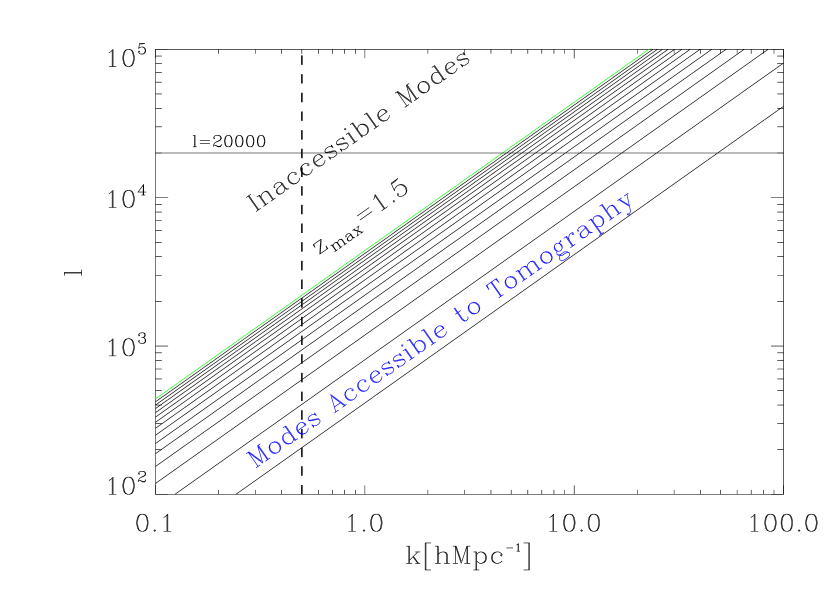
One subtlety, a result of the Limber approximation used in equation (1), and explicitly highlighted by Kitching, Heavens & Miller (2010), is that the radial $k$-modes in the matter power spectrum are associated with the azimuthal $\ell$-modes through $\ell=kr(z)$ where $r(z)$ is the comoving distance for redshift $z$. Commonly angular wavenumbers of up to $\ell_{\rm max}=20$,$000$ are used in theoretical predictions of weak lensing power. If no cut in Fourier 3D wavenumber $k$ is applied for large $\ell$ modes the resulting scales probed in the matter power spectrum can extend into the very highly non-linear regime. For instance for $\ell_{\rm max}=20$,$000$ and $r(z=0.1)=400$Mpc$/h$ we find $k=70h$Mpc^-1, or a physical scale of $126$Kpc$/h$, within the dark matter halo of galaxies. We demonstrate this in Figure 1 where we show the ($\ell$, $k$) plane and the accessible modes, that lie on the lines for a $15$-bin tomography experiment from redshift $0.1$ to $1.5$; it is clear that all modes with $\ell\mathrel{\raise 1.16pt\hbox{$>$}\kern-7.0pt\lower 3.06pt\hbox{{$\scriptstyle\sim$}}}2000$ probe the non-linear regime exclusively.

In this article we will make defined cut in radial $k$-mode, where $k\leq k_{\rm max}$ for all tomographic bins. This allows scales to be probed in a controlled manner so that the non-linear or very non-linear regimes can be removed from the analyses. Equivalently, this can be intepreted as a redshift-dependent $\ell$ cut where $\ell_{\rm max}(z)=k_{\rm max}r(z)$.

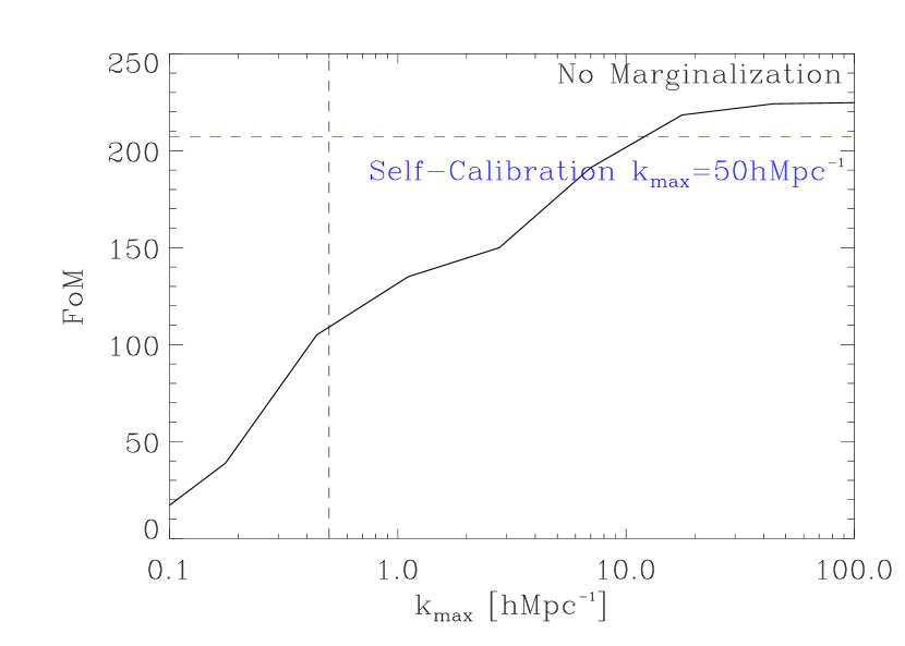
In Figure 2 we show the predicted dark energy Figure of Merit, calculated using a Fisher matrix (Tegmark, Taylor & Heavens, 1997; see Hu 1999 for the cosmic shear tomography Fisher matrix), as a function of the maximum $k$-mode used in the matter power spectrum for a Euclid-like tomographic cosmic shear survey, and a set of cosmological parameters that includes curvature. It is clear that the majority of the dark energy information comes from modes in the non-linear regime (although this statement contains some uncertainty because we have used the Smith et al, 2003 halofit correction).

We find convergence at $k_{\rm max}\approx 50h$Mpc^-1. This is in agreement with previous studies (e.g. Dore, Tingting, Ue-Li, 2009). We can understand the behavior of this plot where the increase in FoM around $k=0.1h$Mpc^-1 corresponds to the nonlinear regime for the matter power-spectrum. The flattening between $k=0.5$ and $k=3h$Mpc^-1 occurs near the linear peak of the matter power spectrum which is less sensitive to dark energy. A second increase in information appears around the peak of the nonlinear regime, and then again saturates at very high $k$.

Figure 1: The $k$ modes that are in principle accessible to a tomographic experiment. As an example we use a $15$ bin tomography experiment with bins at $0.1n$ from $z=0.1$ to $1.5$; solid lines drawn are $\ell=kr(z)$. Tomography uses modes that lie on the lines shown. 3D cosmic shear (Kitching, Heavens, Miller, 2010) would use all modes below the green line, which marks the maximum redshift of the example experiment. The dashed line shows the approximate non-linear cut off of $k\approx 0.5h$Mpc^-1.

Figure 2: The dark energy Figure of Merit (FoM) as a function of the maximum $k$-mode used in the tomographic cosmic shear Fisher matrix analysis for a Euclid-like survey, with no external priors included. The maximum $\ell$ range in the $C(\ell)$ power spectrum is calculated as a function of redshift using $\ell_{\rm max}(z)={\rm min}[k_{\rm max}r(z),2\times 10^{5}]$.

2.3 Path Integral Marginalization

The main issue we are concerned with in this paper is the uncertainty in the shape of the nonlinear matter power spectrum due to baryon effects. In the absence of an accurate estimate of the nonlinear matter power spectrum one can either attempt to self-calibrate it from the cosmic shear data itself, or apply an informative external prior on its shape from hydrodynamical simulations. The self-calibration approach finds the maximum likelihood solution to the free functional nonlinear matter power spectrum using the shear data alone. For a Gaussian likelihood for the matter power spectrum this can be done in a single-step using Newton’s Method or a quadratic estimator (Taylor & Kitching 2010), or iteratively. We then analytically marginalize over all functional forms for the power spectrum permitted by the data, again assuming Gaussian-distributed nonlinear power. The resulting marginalized likelihood function for cosmological parameters is now independent of any initial fiducial choice of the nonlinear matter power, since we have found its maximum likelihood value. This method can be applied to an arbitrary likelihood function for the data, but if we have Gaussian-distributed data, the resulting marginalized likelihood function for the data is again a Gaussian with a new covariance matrix,

$$\mbox{\boldmath$C$}^{M}=[\mbox{\boldmath$C$}^{-1}-\mbox{\boldmath$C$}^{-1}\mbox{\boldmath$P$}\mbox{\boldmath$C$}^{-1}]^{-1}$$ (5)

where $C$ is the orginal covariance and

$$\mbox{\boldmath$P$}=\int\!dx^{\prime}dx^{\prime\prime}\,\frac{\delta\mbox{\boldmath$\mu$}[\psi(x)]}{\delta\psi_{\alpha}(x^{\prime})}F_{\alpha\beta}^{-1}(x^{\prime},x^{\prime\prime})\frac{\delta\mbox{\boldmath$\mu$}^{\dagger}[\psi(x)]}{\delta\psi_{\beta}(x^{\prime\prime})},$$ (6)

for functions $\psi_{\alpha}(x)$, and we assume the functional Fisher matrix, $F_{\alpha\beta}(x,x^{\prime})$ for the function $\psi_{\alpha}(x)$, is invertible. $\mu$ is the mean signal, which in our case is the $C_{ij}(\ell)$ tomographic power spectrum.

If we assume an informative external prior, for example, if we know something about how baryons will affect the matter power spectrum from hydrodynamical simulations, we can include this information by constraining its shape to some accuracy which in general will depend on scale. This additional information can be included in our formalism by multiplying the likelihood with a Gaussian prior with some covariance $C_{\alpha\beta}(x^{\prime},x^{\prime\prime})$. After marginalization, we again find an analytic expression for a general likelihood. In the case of Gaussian-distributed data this also modifies the marginalized covariance, $\mbox{\boldmath$C$}^{M}$. This in turn can be simplified using the Woodbury relation to find that the marginalized data covariance is the original covariance $C$ with a new term added,

$$\mbox{\boldmath$C$}_{M}=\mbox{\boldmath$C$}+\int dx^{\prime}dx^{\prime\prime}\,C_{\alpha\beta}(x^{\prime},x^{\prime\prime})\frac{\delta\mbox{\boldmath$\mu$}[\psi(x)]}{\delta\psi_{\alpha}(x^{\prime})}\frac{\delta\mbox{\boldmath$\mu$}^{t}[\psi(x)]}{\delta\psi_{\beta}(x^{\prime\prime})}.$$ (7)

In the following subsections we derive an expression for the covariance of the tomographic cosmic shear power spectrum in each case. Given the modified covariance $\mbox{\boldmath$C$}^{M}$ a likelihood function can then be constructed that accounts for unknown functional behaviour in the matter power spectrum

$$\mbox{${\cal L}$}_{0}=\Delta D_{\mu}[\mbox{\boldmath$C$}^{M}]_{\mu\nu}^{-1}\Delta D_{\nu}^{t}+{\rm Tr}\,\ln\mbox{\boldmath$C$}^{M},$$ (8)

where $\Delta D_{\mu}=C^{\rm theory}_{ij}(\ell)-C^{\rm data}_{ij}(\ell)$, which could be used in data analysis. We assume a Gaussian likelihood, but in fact any likelihood estimator can be used (see Taylor & Kitching, 2010). For predictive forecasts an associated Fisher matrix can be constructed assuming that the cosmological information is the mean tomographic power spectrum at each redshift

$$F_{ab}=\frac{1}{2}\sum_{\mu\nu}\int\frac{\ell d\ell}{2\pi}\left(\left[\mbox{\boldmath$C$}^{M}_{\mu\nu}(\ell)\right]^{-1}\frac{\partial C_{\mu}(\ell)}{\partial\theta_{a}}\frac{\partial C_{\nu}(\ell)}{\partial\theta_{b}}\right)$$ (9)

for a set of cosmological parameters, $\mn@boldsymbol{\theta}$.

2.4 Self-Calibration

In the self-calibration regime the cosmic shear data itself is used to measure the non-linear power spectrum simultaneously with cosmological parameters. To calculate the impact of this self-calibration we first find the functional derivative of the lensing tomographic power spectrum with respect to the matter power sepctrum, given by

$$\frac{\delta C_{ij,j>i}(\ell)}{\delta P_{\delta\delta}(\ell^{\prime}/r,r)}=W^{GG}_{ij,j>i}(r)\frac{2\pi\delta_{D}(\ell-\ell^{\prime})}{\ell}.$$ (10)

For a flat-prior in function-space over the non-linear matter power spectrum, where we use the data itself to fit and marginalize over uncertainty in the matter power spectrum, the marginalized functional covariance is given by

$$\mbox{\boldmath$C$}^{M}_{\mu\nu}(\ell)=[\mbox{\boldmath$C$}^{-1}_{\mu\nu}(\ell)-\mbox{\boldmath$C$}_{\mu\mu^{\prime}}^{-1}(\ell)\mbox{\boldmath$P$}_{\mu^{\prime}\nu^{\prime}}(\ell)\mbox{\boldmath$C$}^{-1}_{\nu^{\prime}\nu}(\ell)]^{-1}$$ (11)

where

$$\mbox{\boldmath$P$}_{\mu\nu}(\ell)=\int_{0}^{r_{H}}\!\!drdr^{\prime}\,W^{GG}_{\mu}(r)[F(\ell;r,r^{\prime})]^{-1}W^{GG}_{\nu}(r^{\prime}),$$ (12)

and the functional Fisher matrix for the matter power spectrum is

$$F(\ell;r,r^{\prime})=\sum_{\mu\nu}\mbox{\boldmath$C$}^{-1}_{\mu\nu}(\ell)W^{GG}_{\mu}(r)W^{GG}_{\nu}(r^{\prime}).$$ (13)

In practice this functional Fisher matrix is binned in redshift and scale using $200$ bins in each dimension in this paper.

After marginalizing over the nonlinear matter power spectrum, there is still cosmological information in the lensing power spectrum through the lensing kernel. The functional Fisher matrix in equation (13) picks out the geometric dependency of the tomographic cosmic shear power spectrum. Marginalizing over the functional matter power spectrum has some similarity to the geometric shear-ratio test (Jain & Taylor 2003, Taylor et al 2007, Kitching et al 2007), where the shear signal behind galaxy clusters and groups is ratioed, and the mass drops out leaving just the geometric part of the lensing signal. This method can be used in the fully nonlinear clustering regime as there is no sensitivity to clustering.

2.5 External Prior

For an external prior we take the functional derivative of the tomographic cosmic shear power spectrum with respect to the matter power spectrum (equation 10) and, assumming a Gaussian distribution in function-space can now write a covariance for the tomographic cosmic shear power spectrum that marginalizes over all unknown functional behaviour of the matter power spectrum

$$\mbox{\boldmath$C$}^{M}_{\mu\nu}(\ell)=\mbox{\boldmath$C$}_{\mu\nu}(\ell)+\int_{0}^{r_{H}}\!\!{\rm d}r\,\sigma^{2}_{P}(\ell/r,r)W^{GG}_{ij}(r)W^{GG}_{lm}(r),$$ (14)

where $\sigma^{2}_{P}(\ell/r,r)=\langle|\delta P_{\delta\delta}(\ell/r,r)|^{2}\rangle$ is the functional scatter in $P_{\delta\delta}$ and we have assumed the functional covariance is diagonal in $\ell$ and $r$.

3 Results

Here we present cosmic shear Fisher matrix forecasts, marginalizing over uncertainty in the matter power spectrum, for the self-calibration and external prior cases described in Section 2.

3.1 Self-Calibration

In Figure 2 we show the FoM for the case that the matter power spectrum is measured directly from the cosmic shear data, upto a maximum $k=50h$Mpc^-1. We find that relative to the non-marginalization case (where the power is assumed to be known exactly) there is a reduction in the ability of the cosmic shear survey to constrain dark energy parameters by $10\%$. This is equivalent to the maximum $k$-range being reduced from $k=50h$Mpc^-1 to $k\approx 10h$Mpc^-1.

We note that the information in the self-calibration regime comes from the geometric constraints on cosmological parameters that come from the cross-component tomographic bin combinations (for a single bin, with auto-correlation information only the marginalized covariance, equation 11, $\mbox{\boldmath$C$}^{M}\rightarrow\infty$). Because the self-calibration recovers the FoM to within 10% of the unmarginalized case, this suggests that the majority of the dark energy information from cosmic shear tomography, in the non-linear regime, comes from the geometric part of the lensing kernel.

3.2 External Prior

In this section we will place requirements on the functional variance from an external prior on the non-linear power spectrum so that the expected dark energy cosmological constraints remain unaffected. We parameterise the functional variance using

$$\frac{\sigma^{2}_{P}(k,r)}{P^{2}(k,z)}=a_{0}+a_{1}k\,\,\,\,\,\,\,\forall\,\,\,k>0.5h{\rm Mpc}^{-1}$$ (15)

where we will investigate a constant uncertainty and one that scales linearly with the $k$-mode, here $k=\ell/r$ in equation (14). This is an extension of the type of path integral marginalization used in Kitching & Taylor (2010) where only constant functional variances were considered, here we consider varying functional variance. Note that we assume that the variance is not a function of redhift, and that $a_{1}$ has units of $h^{-1}$Mpc.

Figure 3: The dark matter power spectrum at a redshift of zero, as a function of scale. We show 3 examples of the type of $1$-sigma functional variances that can be considered using equation 15. Below $k=0.5h$Mpc^-1 we assume that the power spectrum is known exactly, which extends slightly into the non-linear regime. The horizontal dashed line marks $\Delta^{2}(k)=1$, which is where there is approximately a $1\%$ deviation from linearity. For the calcuations in Section 3 that actual values of $a_{0}$ and $a_{1}$ are an order of magnitude smaller than those shown here, which are are illustrative purposes.

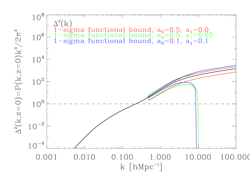
Figure 3 shows an example of the type of functional bounds that we will consider (we show the dimensionless power $\Delta^{2}(k)=P(k)k^{3}/2\pi^{2}$ so that the non-linear regime is marked by $\Delta^{2}(k)\mathrel{\raise 1.16pt\hbox{$>$}\kern-7.0pt\lower 3.06pt\hbox{{$\scriptstyle\sim$}}}1$), throughout we assume that below $k=0.5h$Mpc^-1 the power spectrum is known exactly (zero functional variance) and we take an upper limit in wavenumber of $k\leq k_{\rm max}=50h$Mpc^-1. We use the Eisenstein & Hu (1999) linear power spectrum and the Smith et al. (2003) non-linear correction as the fiducial function.

Figure 4: The FoM, for a Euclid-like tomographic cosmic shear survey alone, as the functional variance of the external prior is varied, as parameterised by equation (15). The FoM degrades as the functional variance is increased. The upper panel shows how the FoM degrades as a functional of $a_{0}$ and $a_{1}$, the lower panel show the dependency on $a_{0}$ keeping $a_{1}=0$. We provide a simple fitting formula (blue, light gray, line) that relates a constant functional variance $a_{0}$ to the FoM. If the functional variance is $\mathrel{\raise 1.16pt\hbox{$<$}\kern-7.0pt\lower 3.06pt\hbox{{$\scriptstyle\sim$}}}0.01$ (vertical dashed line) the FoM is degraded by less than $1\%$. The horizontal dashed line shows the FoM in the self calibration regime.

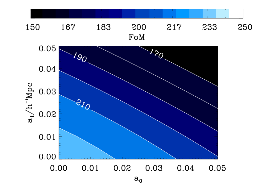
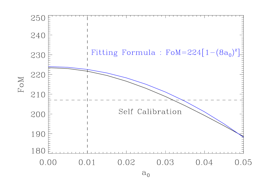
In Figure 4 we show how the FoM for a tomographic cosmic shear, for the survey outlined in Section 2, changes as a function of the functional variance on the non-linear power spectrum from an external prior. We find that if the functional variance can be constrained to $\mathrel{\raise 1.16pt\hbox{$<$}\kern-7.0pt\lower 3.06pt\hbox{{$\scriptstyle\sim$}}}1\%$ then the FoM degradation is at most $1\%$ relative to the case where no marginalization is performed. We provide a simple fitting formula for the dependency of the FoM on the constant contribution to the functional variance

$${\rm FoM}=224[1-(8a_{0})^{2}],$$ (16)

which is valid for $a_{0}\mathrel{\raise 1.16pt\hbox{$<$}\kern-7.0pt\lower 3.06pt\hbox{{$\scriptstyle\sim$}}}0.1$.

4 Conclusion

To conclude we find that the non-linear and baryon-dominated part of the matter power spectrum contains, above wavenumbers of $k\mathrel{\raise 1.16pt\hbox{$>$}\kern-7.0pt\lower 3.06pt\hbox{{$\scriptstyle\sim$}}}0.5h$Mpc^-1, half of the information content on dark energy parameters, parameterised through the Figure of Merit. However the lack of knowledge about this regime, and the complex simulated modelling needed to correctly constrain its behaviour as a function of environment, scale and cosmology means that the uncertainty on the non-linear power spectrum must be correctly accounted for in cosmic shear surveys. This article has some resonance with previous work, that parameterise the uncertainty in the non-linear power spectrum and marginalize over those parameters (Zhang et al., 2009; Rudd et al., 2008; Zenter et al., 2008; Huterer et al., 2006; Jing et al., 2000) or attempt to modify the data to minimise the effect (Huterer & White, 2005), however all these assume parameterized models, that may not be able to reflect the real effect of baryons.

We have derived likelihood expressions for the tomographic cosmic shear power spectrum in the cases that the functional matter power spectrum is self-calibrated from the data itself, and in the case that an external prior on the functional variation of the matter power spectrum is available.

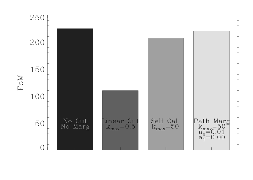
We summarise our results in Figure 5.

• With no external priors, a Euclid-like cosmic shear survey, with a $k_{\rm max}=50h$Mpc^-1 could achieve a FoM $\approx 220$ from cosmic shear tomography alone.
  

• If the non-linear matterpower spectrum is completely removed using a hard cut in $k$-modes of $k_{\rm max}=0.5h$Mpc^-1 then the FoM is reduced by a factor of $50\%$.
  

• In the functional self-calibration regime the cosmic shear survey can recover the FoM, with only a $10\%$ reduction in the FoM.
  

• By including an informative prior, from simulations for example, the orginal FoM can be recovered if the functional variation of the non-linear matter power spectrum is known to $\sim 1\%$ to $k=50h$Mpc^-1, or a physical scale of $\sim 120$Kpc$/h$.

Finally we note that in the self-calibration regime, the information used to constrain the cosmological information, through the lensing kernel, has some similarities with the shear-ratio method, where cluster scale weak lensing is isolated.

Constraining the non-linear power spectrum to 1% functional accuracy down to $120$kpc$/h$ as a function of scale, redshift and cosmology is a significant theoretical and observational challenge. On the theoretical side modeling the baryons on the scale of galaxy clusters is already a challenge. Extending this to group and individual galaxy haloes will require a much deeper understanding of the baryonic processes on these scales. On the observational side, weak lensing itself, and galaxy-galaxy lensing, can provide much empirical information about the mass distribution which can be compared with stellar and gaseous components. These are challenges that must be realised if we are to fully exploit the potential of tomographic cosmic shear experiments.

Figure 5: Summary of the main results. If the non-linear scales are removed using a hard cut in $k$-modes then the FoM can be reduced by $50\%$. In the functional self-calibration regime the reduction is less severe with a relative reduction of $10\%$, finally if a $1\%$ external prior on the functional variation of the non-linear power can be applied then the FoM is recovered. All $k$-modes are in units of $[h$Mpc${}^{-1}]$. The parameters $a_{0}$ and $a_{1}$ refer the shape of the functional variance as a function of scale, given by equation (15).

Acknowledgements: TDK is supported by STFC rolling grant number RA0888. We thank the eScience institute Edinburgh for hosting a workshop on n-body simulations in cosmology. We thank Alan Heavens, Catherine Heymans, Fergus Simpson for interesting discussions on this topic.

References

- [1] Albrecht, A. et al., 2006, eprint arXiv:astro-ph/0609591
- [Bernstein(2009)] Bernstein, G. M. 2009, Astro. Phys. Journal, 695, 652
- [Doré et al.(2009)] Doré, O., Lu, T., & Pen, U.-L. 2009, arXiv:0905.0501
- [Guillet et al.(2010)] Guillet, T., Teyssier, R., & Colombi, S. 2010, MNRAS, 405, 525
- [Heitmann et al.(2010)] Heitmann, K., White, M., Wagner, C., Habib, S., & Higdon, D. 2010, Astro. Phys. Journal, 715, 104
- [Hu(1999)] Hu, W. 1999, Astro. Phys. Journal Letters, 522, L21
- [Huterer et al.(2006)] Huterer, D., Takada, M., Bernstein, G., & Jain, B. 2006, MNRAS, 366, 101
- [Huterer & White(2005)] Huterer, D., & White, M. 2005, Phys. Rev. D, 72, 043002
- [Jing et al.(2006)] Jing, Y. P., Zhang, P., Lin, W. P., Gao, L., & Springel, V. 2006, Astro. Phys. Journal Letters, 640, L119
- [Joachimi & Bridle(2009)] Joachimi, B., & Bridle, S. L. 2009, arXiv:0911.2454
- [Kiessling et al.(2010)] Kiessling, A., Heavens, A. F., & Taylor, A. N. 2010, arXiv:1011.1476
- [Kitching et al.(2008)] Kitching, T. D., Taylor, A. N., & Heavens, A. F. 2008, MNRAS, 389, 173
- [Kitching et al.(2009)] Kitching, T. D., Amara, A., Abdalla, F. B., Joachimi, B.,& Refregier, A. 2009, MNRAS, 399, 2107
- [2] Kitching, T.; Heavens, A.; Miller L.; 2010, arXiv:1007.2953, accepted to MNRAS
- [Kitching et al.(2007)] Kitching, T. D., Heavens, A. F., Taylor, A. N., Brown, M. L., Meisenheimer, K., Wolf, C., Gray, M. E., & Bacon, D. J. 2007, MNRAS, 376, 771
- [Kitching & Taylor(2010)] Kitching, T. D., & Taylor, A. N. 2010, MNRAS, 1564
- [Linder(2003)] Linder, E. V. 2003, Physical Review Letters, 90, 091301
- [Mead et al.(2010)] Mead, J. M. G., King, L. J., Sijacki, D., Leonard, A., Puchwein, E., & McCarthy, I. G. 2010, MNRAS, 406, 434
- [Peacock & Dodds(1996)] Peacock, J. A., & Dodds, S. J. 1996, MNRAS, 280, L19
- [3] Peacock, J. A., & Smith, R. E. 2000, MNRAS, 318, 1144
- [Refregier et al.(2010)] Refregier, A., Amara, A., Kitching, T. D., Rassat, A., Scaramella, R., Weller, J., & Euclid Imaging Consortium, f. t. 2010, arXiv:1001.0061
- [Rudd et al.(2008)] Rudd, D. H., Zentner, A. R., & Kravtsov, A. V. 2008, Astro. Phys. Journal, 672, 19
- [Smith et al.(2003)] Smith, R. E., et al. 2003, MNRAS, 341, 1311
- [4] Taylor A. & Kitching T., 2010, submitted to MNRAS
- [Taylor et al.(2007)] Taylor, A. N., Kitching, T. D., Bacon, D. J., & Heavens, A. F. 2007, MNRAS, 374, 1377
- [Tegmark et al.(1997)] Tegmark, M., Taylor, A. N., & Heavens, A. F. 1997, Astro. Phys. Journal, 480, 22
- [Zentner et al.(2008)] Zentner, A. R., Rudd, D. H., & Hu, W. 2008, Phys. Rev. D, 77, 043507