Adaptive Parallel Tempering for Stochastic Maximum Likelihood Learning of RBMs

Abstract

Restricted Boltzmann Machines (RBM) have attracted a lot of attention of late, as one the principle building blocks of deep networks. Training RBMs remains problematic however, because of the intractibility of their partition function. The maximum likelihood gradient requires a very robust sampler which can accurately sample from the model despite the loss of ergodicity often incurred during learning. While using Parallel Tempering in the negative phase of Stochastic Maximum Likelihood (SML-PT) helps address the issue, it imposes a trade-off between computational complexity and high ergodicity, and requires careful hand-tuning of the temperatures. In this paper, we show that this trade-off is unnecessary. The choice of optimal temperatures can be automated by minimizing average return time (a concept first proposed by [Katzgraber06]) while chains can be spawned dynamically, as needed, thus minimizing the computational overhead. We show on a synthetic dataset, that this results in better likelihood scores.

1 Introduction

Restricted Boltzmann Machines (RBM) [Freund+Haussler-94, Welling05, Hinton06] have become a model of choice for learning unsupervised features for use in deep feed-forward architectures [Hinton06, Bengio-2009] as well as for modeling complex, high-dimensional distributions [Welling05, TaylorHintonICML2009, Larochelle+al-2010]. Their success can be explained in part through the bi-partite structure of their graphical model. Units are grouped into a visible layer $\mathbf{v}$ and a hidden layer $\mathbf{h}$, prohibiting connections within the same layer. The use of latent variables affords RBMs a rich modeling capacity, while the conditional independence property yields a trivial inference procedure.

RBMs are parametrized by an energy function ${\bf E}(\mathbf{v},\mathbf{h})$ which is converted to probability through the Boltzmann distribution, after marginalizing out the hidden units. The probability of a given configuration $p(\mathbf{v})$ is thus given by $p(\mathbf{v})=\frac{1}{Z}\sum_{\mathbf{h}}\exp(-{\bf E}(\mathbf{v},\mathbf{h}))$, where $Z$ is the partition function defined as $Z=\sum_{\mathbf{v},\mathbf{h}}\exp(-{\bf E}(\mathbf{v},\mathbf{h}))$.

Despite their popularity, direct learning of these models through maximum likelihood remains problematic. The maximum likelihood gradient with respect to the parameters $\theta$ of the model is:

$$\frac{\partial\log p(\mathbf{v})}{\partial\theta} = -\sum_{\mathbf{h}}p(\mathbf{h}|\mathbf{v})\frac{\partial{\bf E}(\mathbf{v},\mathbf{h})}{\partial\theta}+\sum_{\mathbf{v^{{\bf-}}},\mathbf{h^{{\bf-}}}}p(\mathbf{v^{{\bf-}}},\mathbf{h^{{\bf-}}})\frac{\partial{\bf E}(\mathbf{v^{{\bf-}}},\mathbf{h^{{\bf-}}})}{\partial\theta}$$ (1)

The first term is trivial to calculate and is referred to as the positive phase, as it raises the probability of training data. The second term or negative phase is intractable in most applications of interest, as it involves an expectation over $p(\mathbf{v},\mathbf{h})$. Many learning algorithms have been proposed in the literature to address this issue:

• Contrastive Divergence (CD) [Hinton99, Hinton2002] replaces the expectation with a finite set of negative samples, which are obtained by running a short Markov chain initialized at positive training examples. This yields a biased, but low-variance gradient which has been shown to work well as a feature extractor for deep networks such as the Deep Belief Network [Hinton06].

• Stochastic Maximum Likelihood (SML) or Persistent Contrastive Divergence (PCD) [Younes98onthe, Tieleman08] on the other hand, relies on a persistent Markov chain to sample the negative particles. The chain is run for a small number of steps between consecutive model updates, with the assumption that the Markov chain will stay close to its equilibrium distribution as the parameters evolve. Learning actually encourages this process, in what is called the “fast-weight effect” [TielemanT2009].

• Ratio Matching and Score Matching [Hyvarinen-2005, Hyvarinen-2007] avoid the issue of the partition function altogether by replacing maximum likelihood by another learning principle, based on matching the change in likelihood to that implied by the empirical distribution.

[Marlin10InductivePrinciples] recently compared these algorithms on a variety of tasks and found SML to be the most attractive method when taking computational complexity into account. Unfortunately, these results fail to address the main shortcomings of SML. First, it relies on Gibbs sampling to extract negative samples: a poor choice when sampling from multi-modal distributions. Second, to guarantee convergence, the learning rate must be annealed throughout learning in order to offset the loss of ergodicity incurred by the Markov chain due to parameter updates [Younes98onthe, Desjardins+al-2010]. Using tempering in the negative phase of SML [Desjardins+al-2010, Cho10IJCNN, Salakhutdinov-2010, Salakhutdinov-ICML2010] appears to address these issues to some extent. By performing a random walk in the joint (configuration, temperature) space, negative particles can escape regions of high probability and travel between disconnected modes. Also, since high temperature chains are inherently more ergodic, the sampler as a whole exhibits better mixing and results in better convergence properties than traditional SML.

Tempering is still no panacea however. Great care must be taken to select the set of temperatures ${\bf\mathcal{T}}=\{T_{1},...,T_{M};T_{1}<T_{i}<T_{M}\ \forall i\in[1,M],M\in\mathbb{N}\}$ over which to run the simulation. Having too few or incorrectly spaced chains can result in high rejection ratios (tempered transition), low return rates (simulated tempering) or low swap rates between neighboring chains (parallel tempering), which all undermine the usefulness of the method. In this work, we show that the choice of ${\bf\mathcal{T}}$ can be automated for parallel tempering, both in terms of optimal temperature spacing, as well as the number of chains to simulate. Our algorithm relies heavily on the work of [Katzgraber06], who were the first to show that optimal temperature spacing can be obtained by minimizing the average return time of particles under simulation.

The paper is organized as follows. We start with a brief review of SML, then explore the details behind SML with Parallel Tempering (SML-PT) as described in [Desjardins+al-2010]. Following this, we show how the algorithm of Katzgraber et al. can be adapted to the online gradient setting for use with SML-PT and show how chains can be created dynamically, so as to maintain a given level of ergodicity throughout training. We then proceed to show various results on a complex synthetic dataset.

2 SML with Optimized Parallel Tempering

2.1 Parallel Tempered SML (SML-PT)

We start with a very brief review of SML, which will serve mostly to anchor our notation. For details on the actual algorithm, we refer the interested reader to [TielemanT2009, Marlin10InductivePrinciples]. RBMs are parametrized by $\theta=\{\mathbf{W},\mathbf{b},\mathbf{c}\}$, where $\mathbf{b}_{i}$ is the $i$-th hidden bias, $\mathbf{c}_{j}$ the $j$-th visible bias and $W_{ij}$ is the weight connecting units $h_{i}$ to $v_{j}$. They belong to the family of log-linear models whose energy function is given by ${\bf E}(\mathbf{x})=-\sum_{k}\theta_{k}\phi_{k}(\mathbf{x})$, where $\phi_{k}$ are functions associated with each parameter $\theta_{k}$. In the case of RBMs, $\mathbf{x}=(\mathbf{v},\mathbf{h})$ and $\phi(\mathbf{v},\mathbf{h})=(\mathbf{h}\mathbf{v}^{T},\mathbf{h},\mathbf{v})$. For this family of model, the gradient of Equation 1 simplifies to:

$$\frac{\partial\log p(\mathbf{v})}{\partial\theta} = \mathbb{E}_{p(\mathbf{h}|\mathbf{v})}[\phi(\mathbf{v},\mathbf{h})]-\mathbb{E}_{p(\mathbf{v},\mathbf{h})}[\phi(\mathbf{v},\mathbf{h})].$$ (2)

As was mentioned previously, SML approximates the gradient by drawing negative phase samples (i.e. to estimate the second expectation) from a persistent Markov chain, which attempts to track changes in the model. If we denote the state of this chain at timestep $t$ as $\mathbf{v}^{-}_{t}$ and the i-th training example as $\mathbf{v}^{(i)}$, then the stochastic gradient update follows $\phi(\mathbf{v}^{(i)},\tilde{\mathbf{h}})-\phi(\tilde{\mathbf{v}}^{-}_{t+k},\tilde{\mathbf{h}}^{-}_{t+k})$, where $\tilde{\mathbf{h}}=\mathbb{E}[\mathbf{h}|\mathbf{v}=\mathbf{v}^{(i)}]$, and $\tilde{\mathbf{v}}^{-}_{t+k}$ is obtained after $k$ steps of alternating Gibbs starting from state $\mathbf{v}^{-}_{t}$ and $\tilde{\mathbf{h}}^{-}_{t+k}=\mathbb{E}[\mathbf{h}|\mathbf{v}=\mathbf{v}^{-}_{t+k}]$.

Training an RBM using SML-PT maintains the positive phase as is. During the negative phase however, we create and sample from an an extended set of $M$ persistent chains, $\{p_{\beta_{i}}(\mathbf{v},\mathbf{h})|i\in[1,M],\beta_{i}\geq\beta_{j}\iff i<j\}$. Here each $p_{\beta_{i}}(\mathbf{v},\mathbf{h})=\frac{\exp(-\beta_{i}{\bf E}(\mathbf{x}))}{Z(\beta_{i})}$ represents a smoothed version of the distribution we wish to sample from, with the inverse temperature $\beta_{i}=1/T_{i}\in[0,1]$ controlling the degree of smoothing. Distributions with small $\beta$ values are easier to sample from as they exhibit greater ergodicity.

After performing $k$ Gibbs steps for each of the $M$ intermediate distributions, cross-temperature state swaps are proposed between neighboring chains using a Metropolis-Hastings-based swap acceptance criterion. If we denote by $\mathbf{x}_{i}$ the joint state (visible and hidden) of the $i$-th chain, the swap acceptance ratio $r_{i}$ for swapping chains ($i$,$i+1$) is given by:

$$r_{i} =\max(1,\frac{p_{\beta_{i}}(\mathbf{x}_{i+1})p_{\beta_{i+1}}(\mathbf{x}_{i})}{p_{\beta_{i}}(\mathbf{x}_{i})p_{\beta_{i+1}}(\mathbf{x}_{i+1})})$$ (3)

Although one might reduce variance by using free-energies to compute swap ratios, we prefer using energies as the above factorizes nicely into the following expression:

$$r_{i}=\exp((\beta_{i}-\beta_{i+1})\cdot({\bf E}(\mathbf{x}_{i})-{\bf E}(\mathbf{x}_{i+1}))),$$ (4)

While many swapping schedules are possible, we use the Deterministic Even Odd algorithm (DEO) [Lingenheil200980], described below.

2.2 Return Time and Optimal Temperatures

Conventional wisdom for choosing the optimal set ${\bf\mathcal{T}}$ has relied on the “flat histogram” method which selects the parameters $\beta_{i}$ such that the pair-wise swap ratio $r_{i}$ is constant and independent of the index $i$. Under certain conditions (such as when sampling from multi-variate Gaussian distributions), this can lead to a geometric spacing of the temperature parameters [Neal94b]. [Behrens2010] has recently shown that geometric spacing is actually optimal for a wider family of distributions characterized by $\mathbb{E}_{\beta}({\bf E}(x))=K_{1}/\beta+K_{2}$, where $\mathbb{E}_{\beta}$ denotes the expectation over inverse temperature and $K_{1},K_{2}$ are arbitrary constants.

Since this is clearly not the case for RBMs, we turn to the work of [Katzgraber06] who propose a novel measure for optimizing ${\bf\mathcal{T}}$. Their algorithm directly maximizes the ergodicity of the sampler by minimizing the time taken for a particle to perform a round-trip between $\beta_{1}$ and $\beta_{M}$. This is defined as the average “return time” $\tau_{rt}$. The benefit of their method is striking: temperatures automatically pool around phase transitions, causing spikes in local exchange rates and maximizing the “flow” of particles in temperature space.

The algorithm works as follows. For $N_{s}$ sampling updates:

• assign a label to each particle: those swapped into $\beta_{1}$ are labeled as “up” particles. Similarly, any “up” particle swapped into $\beta_{M}$ becomes a “down” particle.

• after each swap proposal, update the histograms $n_{u}(i),n_{d}(i)$, counting the number of “up” and “down” particles for the Markov chain associated with $\beta_{i}$.

• define $f_{up}(i)=\frac{n_{u}(i)}{n_{u}(i)+n_{d}(i)}$, the fraction of “up”-moving particles at $\beta_{i}$. By construction, notice that $f_{up}(\beta_{1})=1$ and $f_{up}(\beta_{M})=0$. $f_{up}$ thus defines a probability distribution of “up” particles in the range $[\beta_{1},\beta_{M}]$.

• The new inverse temperature parameters $\beta^{\prime}$ are chosen as the ordered set which assigns equal probability mass to each chain. This yields an $f_{up}$ curve which is linear in the chain index.

The above procedure is applied iteratively, each time increasing $N_{s}$ so as to fine-tune the $\beta_{i}$’s. To monitor return time, we can simply maintain a counter $\tau_{i}$ for each particle $\mathbf{x}_{i}$, which is (1) incremented at every sampling iteration and (2) reset to 0 whenever $\mathbf{x}_{i}$ has label “down” and is swapped into $\beta_{1}$. A lower-bound for return time is then given by ${\hat{\tau}_{rt}}=\sum_{i=0}^{M}\tau_{i}$.

2.3 Optimizing ${\bf\mathcal{T}}$ while Learning

2.3.1 Online Beta Adaptation

While the above algorithm exhibits the right properties, it is not very well suited to the context of learning. When training an RBM, the distribution we are sampling from is continuously changing. As such, one would expect the optimal set ${\bf\mathcal{T}}$ to evolve over time. We also do not have the luxury of performing $N_{s}$ sampling steps after each gradient update.

Our solution is simple: the histograms $n_{u}$ and $n_{d}$ are updated using an exponential moving average, whose time constant is in the order of the return time $\hat{\tau}_{rt}$. Using $\hat{\tau}_{rt}$ as the time constant is crucial as it allows us to maintain flow statistics at the proper timescale. If an “up” particle reaches the $i$-th chain, we update $n_{u}(i)$ as follows:

$$n_{u}^{t+1}(i)=n_{u}^{t}(i)(1-1/{\hat{\tau}_{rt}^{t}})+1/{\hat{\tau}_{rt}^{t}},$$ (5)

where $\hat{\tau}_{rt}^{t}$ is the estimated return time at time $t$.

Using the above, we can estimate the set of optimal inverse temperatures $\beta_{i}^{\prime}$. Beta values are updated by performing a step in the direction of the optimal value: $\beta_{i}^{t+1}=\beta_{i}^{t}+\mu(\beta_{i}^{\prime}-\beta_{i}^{t})$, where $\mu$ is a learning rate on $\beta$. The properties of [Katzgraber06] naturally enforce the ordering constraint on the $\beta_{i}$’s.

2.3.2 Choosing $M$ and $\beta_{M}$

Another important point is that [Katzgraber06] optimizes the set ${\bf\mathcal{T}}$ while keeping the bounds $\beta_{1}$ and $\beta_{M}$ fixed. While $\beta_{1}=1$ is a natural choice, we expect the optimal $\beta_{M}$ to vary during learning. For this reason, we err on the side of caution and use $\beta_{M}=0$, relying on a chain spawning process to maintain sufficiently high swap rates between neighboring parallel chains. Spawning chains as required by the sampler should therefore result in increased stability, as well as computational savings.

[Lingenheil200980] performed an interesting study where they compared the round trip rate $1/\tau_{rt}$ to the average swap rate measured across all chains. They found that the DEO algorithm, which alternates between proposing swaps between chains $\{(i,i+1);\forall\,{\rm even}\,i\}$ followed by $\{(i,i+1);\forall\,{\rm odd}\,i\}$), gave rise to a concave function with a broad maximum around an average swap rate of $\bar{r}=\sum_{i}{r_{i}}\approx 0.4$

Our temperature adaptation therefore works in two phases:

1. The algorithm of Katzgraber et. al is used to optimize $\{\beta_{i};1<i<M\}$, for a fixed M.

2. Periodically, a chain is spawned whenever $\bar{r}<\bar{r}_{min}$, a hyper-parameter of the algorithm.

Empirically, we have observed increased stability when the index $j$ of the new chain is selected such that $j=\mathrm{argmax}_{i}(|f_{up}(i)-f_{up}(i+1)|)$, $i\in[1,M-1]$. To avoid a long burn-in period, we initialize the new chain with the state of the $(j+1)$-th chain and choose its inverse temperature as the mean $(\beta_{j}+\beta_{j+1})/2$. A small but fixed burn-in period allows the system to adapt to the new configuration.

3 Results and Discussion

We evaluate our adaptive SML-PT algorithm (SML-APT) on a complex, synthetic dataset. This dataset is heavily inspired from the one used in [Desjardins+al-2010] and was specifically crafted to push the limits of the algorithm.

It is an online dataset of $28$x$28$ binary images, where each example is sampled from a mixture model with probability density function $f_{X}(x)=\sum_{m=1}^{5}w_{m}f_{Y_{m}}(x)$. Our dataset thus consists of $5$ mixture components whose weights $w_{m}$ are sampled uniformly in the unit interval and normalized to one. Each mixture component $Y_{m}$ is itself a random $28$x$28$ binary image, whose pixels are independent random variables having a probability $p_{m}$ of being flipped. From the point of view of a sampler performing a random walk in image space, $p_{m}$ is inversely proportional to the difficulty of finding the mode in question. The complexity of our synthetic dataset comes from our particular choice of $w_{m}$ and $p_{m}$. Large $w_{m}$ and small $p_{m}$ lead to modes which are difficult to sample and in which a Gibbs sampler would tend to get trapped. Large $p_{m}$ values on the other hand will tend to intercept ”down” moving particles and thus present a challenge for parallel tempering.

Figure 1(a) compares the results of training a $10$ hidden unit RBM, using standard SML, SML-PT with $\{10,20,50\}$ parallel chains and our new SML-APT algorithm. We performed $10^{5}$ updates (followed by $2\cdot 10^{4}$ steps of sampling) with mini-batches of size 5 and tested learning rates in $\{10^{-3},10^{-4}\}$, $\beta$ learning rates in $\{10^{-3},10^{-4},10^{-5}\}$. For each algorithm, we show the results for the best performing hyper-parameters, averaging over $5$ different runs. Results are plotted with respect to computation time to show the relative computational cost of each algorithm.

(a) Log-likelihood

(b) Return Time

Figure 1: (a) Comparison of training likelihood as a function of time for standard SML, SML-PT with 10/20/50 chains and the proposed SML-APT (initialized with 10 chains). SML-APT adapts the temperature set ${\bf\mathcal{T}}=\{T_{1},...,T_{M};T_{1}<T_{i}<T_{M}\}$ to minimize round trip time between chains $T_{1}$ and $T_{M}$, and modifies the number of chains $M$ to maintain a minimal average swap rate. The resulting sampler exhibits greater ergodicity and yields better likelihood scores than standard SML and SML-PT, without requiring a careful hand-tuning of ${\bf\mathcal{T}}$. (b) Average return time of each algorithm. SML-APT successfully minimizes this metric resulting in a return time similar to SML-PT 10, while still outperforming SML-PT $50$ in terms of likelihood. Errors bars represent standard error on the mean.

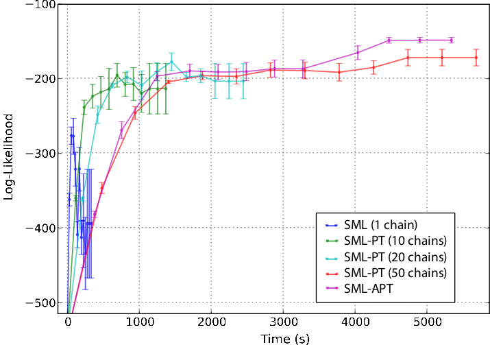
As we can see, standard SML fails to learn anything meaningful: the Gibbs sampler is unable to cope with the loss in ergodicity and the model diverges. SML-PT on the other hand performs much better. Using more parallel chains in SML-PT consistently yields a better likelihood score, as well as reduced variance. This seems to confirm that using more parallel chains in SML-PT increases the ergodicity of the sampler. Finally, SML-APT outperforms all other methods. As we will see in Figure 2, it does so using only $20$ parallel chains. Unfortunately, the computational cost seems similar to 50 parallel chains. We hope this can be reduced to the same cost as SML-PT with $20$ chains in the near future. Also interesting to note, while the variance of all methods increase with training time, SML-APT seems immune to this issue.

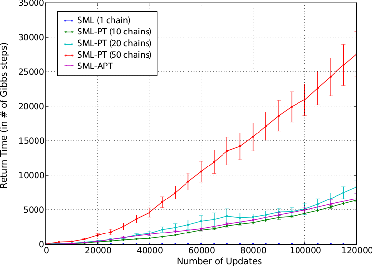
We now compare the various metrics being optimized by our adaptive algorithm. Figure 1(b) shows the average return time for each of the algorithms. We can see that SML-APT achieves a return time which is comparable to SML-PT with 10 chains, while achieving a better likelihood score than SML-PT 50.

We now select the best performing seeds for SML-PT with 50 chains and SML-APT, and show in Figure 2, the resulting $f_{up}(i)$ curves obtained at the end of training.

(a) SML-APT

(b) SML-PT 50

Figure 2: Return time is minimized by tagging each particle with a label: “up” if the particle visited $T_{1}$ more recently than $T_{M}$ and “down” otherwise. Histograms $n_{u}(i)$ and $n_{d}(i)$ track the number of up/down particles at each temperature $T_{i}$. Temperatures are modified such that the ratio $f_{up}(i)=n_{u}(i)/(n_{u}(i)+n_{d}(i))$ is linear in the index $i$. (a) $f_{up}$ curve obtained with SML-APT, as a function of temperature index (blue) and inverse temperature (red). SML-APT achieves a linear $f_{up}$ in the temperature index $i$. (b) Typical $f_{up}$ curve obtained with SML-PT (here using 50 chains). $f_{up}$ is not linear in the index $i$, which translates to larger return times as shown in Fig. 1(b).

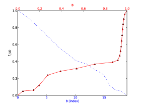
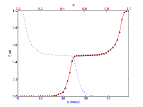
The blue curve plots $f_{up}$ as a function of beta index, while the red curves plots $f_{up}$ as a function of $\beta$. We can see that SML-APT results in a more or less linear curve for $f_{up}(i)$, which is not the case for SML-PT. In Figure 3(a) we can see the effect on the pair-wise swap statistics $r_{i}$. As reported in [Katzgraber06], optimizing ${\bf\mathcal{T}}$ to maintain a linear $f_{up}$ leads to temperatures pooling around the bottleneck. In comparison, SML-PT fails to capture this phenomenon regardless of whether it uses $20$ or $50$ parallel chains (figures 3(b)-3(c)).

(a) SML-APT

(b) SML-PT 20

(c) SML-PT 50

Figure 3: Pairwise swap statistics obtained after $10^{5}$ updates. Minimizing return time causes SML-APT to pool temperatures around bottlenecks, achieving large swap rates (0.9) around bottenecks with relatively few chains. SML-PT on the other hand results in a much flatter distribution, requiring around 50 chains to reach swap rates close to 0.8.

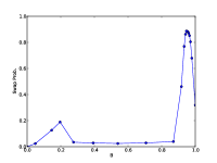
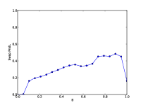
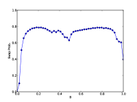
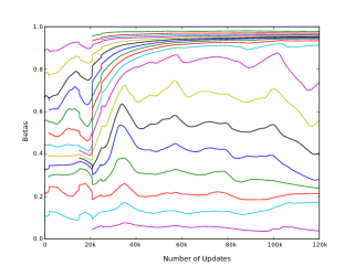
Finally, Figure 4 shows the evolution of the inverse temperature parameters throughout learning. We can see that the position of the bottleneck in temperature space changes with learning. As such, a manual tuning of temperatures would be hopeless in achieving optimal return times.

Figure 4: Graphical depiction of the set $\{\beta_{i};i\in[1,M]\}$, of inverse temperature parameters used by SML-APT during learning. Temperatures pool around a bottleneck to minimize return time, while new chains are spawned to maintain a given average swap rate. Note that the last $20$k updates actually correspond to a pure sampling phase (i.e. a learning rate of 0).

4 Conclusion

We have introduced a new adaptive training algorithm for RBMs, which we call Stochastic Maximum Likelihood with Adaptive Parallel Tempering (SML-APT). It leverages the benefits of PT in the negative phase of SML, but adapts and spawns new temperatures so as to minimize return time. The resulting negative phase sampler thus exhibits greater ergodicity. Using a synthetic dataset, we have shown that this can directly translate to a better and more stable likelihood score. In the process, SML-APT also greatly reduces the number of hyper-parameters to tune: temperature set selection is not only automated, but optimal. The end-user is left with very few dials: a standard learning rate on $\beta_{i}$ and a minimum average swap rate $\bar{r}_{min}$ below which to spawn.

Much work still remains. In terms of computational cost, we would like a model trained with SML-APT and resulting in $M$ chains, to always be upper-bounded by SML-PT initialized with $M$ chains. Obviously, the above experiments should also be repeated with larger RBMs on natural datasets, such as MNIST or Caltech Silhouettes..

Acknowledgments

The authors acknowledge the support of the following agencies for research funding and computing support: NSERC, Compute Canada and CIFAR. We would also like to thank the developers of Theano , for developing such a powerful tool for scientific computing, especially gradient-based learning.

References

- Behrens et al., 2010 Behrens et al.][2010]Behrens2010 Behrens, G., Friel, N., & Hurn, M. (2010). Tuning Tempered Transitions. ArXiv e-prints.
- Bengio, 2009 Bengio][2009]Bengio-2009 Bengio, Y. (2009). Learning deep architectures for AI. Foundations and Trends in Machine Learning, 2, 1–127. Also published as a book. Now Publishers, 2009.
- Cho et al., 2010 Cho et al.][2010]Cho10IJCNN Cho, K., Raiko, T., & Ilin, A. (2010). Parallel tempering is efficient for learning restricted boltzmann machines. Proceedings of the International Joint Conference on Neural Networks (IJCNN 2010). Barcelona, Spain.
- Desjardins et al., 2010 Desjardins et al.][2010]Desjardins+al-2010 Desjardins, G., Courville, A., & Bengio, Y. (2010). Tempered Markov chain monte carlo for training of restricted Boltzmann machine. Proceedings of AISTATS 2010 (pp. 145–152).
- Freund & Haussler, 1994 Freund and Haussler][1994]Freund+Haussler-94 Freund, Y., & Haussler, D. (1994). Unsupervised learning of distributions on binary vectors using two layer networks (Technical Report UCSC-CRL-94-25). University of California, Santa Cruz.
- Hinton, 1999 Hinton][1999]Hinton99 Hinton, G. E. (1999). Products of experts. Proceedings of the Ninth International Conference on Artificial Neural Networks (ICANN) (pp. 1–6). Edinburgh, Scotland: IEE.
- Hinton, 2002 Hinton][2002]Hinton2002 Hinton, G. E. (2002). Training products of experts by minimizing contrastive divergence. Neural Computation, 14, 1771–1800.
- Hinton et al., 2006 Hinton et al.][2006]Hinton06 Hinton, G. E., Osindero, S., & Teh, Y. (2006). A fast learning algorithm for deep belief nets. Neural Computation, 18, 1527–1554.
- Hyvärinen, 2005 Hyvärinen][2005]Hyvarinen-2005 Hyvärinen, A. (2005). Estimation of non-normalized statistical models using score matching. Journal of Machine Learning Research, 6, 695–709.
- Hyvärinen, 2007 Hyvärinen][2007]Hyvarinen-2007 Hyvärinen, A. (2007). Some extensions of score matching. Computational Statistics and Data Analysis, 51, 2499–2512.
- Katzgraber et al., 2006 Katzgraber et al.][2006]Katzgraber06 Katzgraber, H. G., Trebst, S., Huse, D. A., & Troyer, M. (2006). Feedback-optimized parallel tempering monte carlo. Journal of Statistical Mechanics: Theory and Experiment, 2006, P03018.
- Larochelle et al., 2010 Larochelle et al.][2010]Larochelle+al-2010 Larochelle, H., Bengio, Y., & Turian, J. (2010). Tractable multivariate binary density estimation and the restricted Boltzmann forest. Neural Computation, 22, 2285–2307.
- Lingenheil et al., 2009 Lingenheil et al.][2009]Lingenheil200980 Lingenheil, M., Denschlag, R., Mathias, G., & Tavan, P. (2009). Efficiency of exchange schemes in replica exchange. Chemical Physics Letters, 478, 80 – 84.
- Marlin et al., 2010 Marlin et al.][2010]Marlin10InductivePrinciples Marlin, B., Swersky, K., Chen, B., & de Freitas, N. (2010). Inductive principles for restricted boltzmann machine learning. In Proceedings of the Thirteenth International Conference on Artificial Intelligence and Statistics (AISTATS 2010).
- Nadler & Hansmann, 2007 Nadler and Hansmann][2007]Nadler07 Nadler, W., & Hansmann, U. H. E. (2007). Generalized ensemble and tempering simulations: A unified view. Phys. Rev. E, 75, 026109.
- Neal, 1994 Neal][1994]Neal94b Neal, R. M. (1994). Sampling from multimodal distributions using tempered transitions (Technical Report 9421). Dept. of Statistics, University of Toronto.
- Salakhutdinov, 2010a Salakhutdinov][2010a]Salakhutdinov-ICML2010 Salakhutdinov, R. (2010a). Learning deep boltzmann machines using adaptive mcmc. Proceedings of the Twenty-seventh International Conference on Machine Learning (ICML-10) (pp. 943–950). ACM.
- Salakhutdinov, 2010b Salakhutdinov][2010b]Salakhutdinov-2010 Salakhutdinov, R. (2010b). Learning in Markov random fields using tempered transitions. NIPS’09.
- Taylor & Hinton, 2009 Taylor and Hinton][2009]TaylorHintonICML2009 Taylor, G., & Hinton, G. (2009). Factored conditional restricted Boltzmann machines for modeling motion style. Proceedings of the 26th International Conference on Machine Learning (ICML’09) (pp. 1025–1032). Montreal: Omnipress.
- Tieleman, 2008 Tieleman][2008]Tieleman08 Tieleman, T. (2008). Training restricted boltzmann machines using approximations to the likelihood gradient. ICML 2008 (pp. 1064–1071). Helsinki, Finland: ACM.
- Tieleman & Hinton, 2009 Tieleman and Hinton][2009]TielemanT2009 Tieleman, T., & Hinton, G. (2009). Using fast weights to improve persistent contrastive divergence. ICML 2009 (pp. 1033–1040). ACM.
- Welling et al., 2005 Welling et al.][2005]Welling05 Welling, M., Rosen-Zvi, M., & Hinton, G. E. (2005). Exponential family harmoniums with an application to information retrieval. NIPS’04. Cambridge, MA: MIT Press.
- Younes, 1998 Younes][1998]Younes98onthe Younes, L. (1998). On the convergence of markovian stochastic algorithms with rapidly decreasing ergodicity rates. Stochastics and Stochastics Models (pp. 177–228).