Characterization and quantification of the role of coherence in ultrafast quantum biological experiments using quantum master equations, atomistic simulations, and quantum process tomography

Abstract

Long-lived electronic coherences in various photosynthetic complexes at cryogenic and room temperature have generated vigorous efforts both in theory and experiment to understand their origins and explore their potential role to biological function. The ultrafast signals resulting from the experiments that show evidence for these coherences result from many contributions to the molecular polarization. Quantum process tomography (QPT) is a technique whose goal is that of obtaining the time-evolution of all the density matrix elements based on a designed set of experiments with different preparation and measurements. The QPT procedure was conceived in the context of quantum information processing to characterize and understand general quantum evolution of controllable quantum systems, for example while carrying out quantum computational tasks. We introduce our QPT method for ultrafast experiments, and as an illustrative example, apply it to a simulation of a two-chromophore subsystem of the Fenna-Matthews-Olson photosynthetic complex, which was recently shown to have long-lived quantum coherences. Our Fenna-Matthews-Olson model is constructed using an atomistic approach to extract relevant parameters for the simulation of photosynthetic complexes that consists of a quantum mechanics/molecular mechanics approach combined with molecular dynamics and the use of state-of-the-art quantum master equations. We provide a set of methods that allow for quantifying the role of quantum coherence, dephasing, relaxation and other elementary processes in energy transfer efficiency in photosynthetic complexes, based on the information obtained from the atomistic simulations, or, using QPT, directly from the experiment. The ultimate goal of the combination of this diverse set of methodologies is to provide a reliable way of quantifying the role of long-lived quantum coherences and obtain atomistic insight of their causes.

I Introduction

The initial step in photosynthesis is highly efficient excitonic transport of the energy captured from photons to a reaction center Blankenship2002 . In most plants and photosynthetic organisms this process occurs in light-harvesting complexes which are interacting chlorophyll molecules embedded in a solvent and a protein environment Cheng2009 . Several recent experiments show that excitonic coherence can persist for several hundreds of femtoseconds even at physiological temperature Engel2007 ; Lee2007 ; Panitchayangkoon2010 ; Collini2010 . These experiments suggest the hypothesis that quantum coherence is biologically relevant for photosynthesis. The results have motivated a sizeable amount of recent theoretical work regarding the reasons for the long-lived coherences and their role to the function.

The focus of many studies is on the theoretical models employed. In this context, it is essential to be as realistic an possible and employ the least amount of approximations. Most of the currently-employed methods involve a master equation for the reduced excitonic density operator where the vibrational degrees of freedom (phonons) of the protein and solvent are averaged out. Amongst these simple methods are the Haken-Strobl model and Redfield theory as employed in Refs. Rebentrost2009b ; Plenio2008 and Mohseni2008 respectively. To interpolate between the usual weak and strong exciton-phonon coupling limits, Ishizaki and Fleming developed a hierarchical equation of motion (HEOM) theory which takes into account non-equilibrium molecular reorganization effects Ishizaki2009 . Jang et al. perform a second order time-convolutionless expansion after a small polaron transformation to include strong coupling effects Jang2008 .Another set of studies focuses on the role of quantum coherence and the phonon environmentin terms of transport efficiency or entanglement. It was shown that the transport efficiency is enhanced by the interaction or interplay of the quantum evolution with the phononic environment Rebentrost2009b ; Plenio2008 ; Mohseni2008 ; Wu2010 . Entanglement between molecules is found to persist for long times Sarovar2010 ; Caruso2010a ; Fassioli2010 .

The ongoing effort can be summarized with two equally important questions: What are the microscopic reasons for the persistence of quantum coherence and what is the relevance of the quantum effect to the biological functionality of the organism under study? In this work, we summarize the recent efforts from our group to approach the problem from several angles. Firstly, we investigate the role of coherences in the exciton transfer process of the Fenna-Matthews-Olson (FMO) complex. We quantify the amount and the contribution of coherence to the efficient energy transfer process. Secondly, we present our quantum mechanics/molecular mechanics (QM/MM) approach to obtain information about the system at the atomistic level, such as detailed bath dynamics and spectral densities. Finally, we propose a spectroscopic tool that allows for obtaining directly the information of the quantum process via our recent theoretical proposal for the quantum process tomography technique to the ultrafast regime.

II The Role of Quantum Coherence

In this section, we discuss the question about the relevance of quantum effects to the biological function. A negative answer to this question would mean that a particular effect, while being quantum, is not leading to any improvement in the functionality of a biological system, and therefore would be a byproduct of the spatial and temporal scales and physical properties of the problem. For example, in energy transfer (ET) quantum coherence could arise from the closely packed arrangement of the chromophores in a protein scaffold but it could, in principle, represent a byproduct of that arrangement and not a relevant feature. Another example, it may be true that the human eye can detect a single photon, but it is not clear if this quantum effect is relevant to the biological function, which usually operates at much larger photon fluxes. If, on the other hand, the above yes-no question of the relevance is answered positively for a particular effect in a biological system, it would present a major step towards establishing the relevance or importance of a quantum biological phenomenon. A natural follow-up questions is: How important quantitatively is a particular quantum effect?

Both of these questions should preferably be studied by experimental means. An experiment would have to be designed in a way that tests for the biological relevance of quantum coherence. Possible experiments could involve quantum measurements on mutated samples. In the FMO complex that acts as a molecular ET wire the efficiency of the transport event is most likely a good quantifier for biological function. One would need a way to experimentally quantify this efficiency and extract the relevance of quantum coherence to the efficiency. This can be hard in practice. Yet, as we will discuss in this work, quantum process tomography is able to obtain detailed information about quantum coherence and the phonon environment and might thus lead to progress in this area.

In the case when experimental access to an observable that involves the biological relevance is hard or impossible, a theoretical treatment can provide insight. It is illustrative to analyze a model of the particular biological process in terms of a quantifier for the success of the process. An example is the aforementioned efficiency of energy transport. In bird vision, the quantum yield of a chemical reaction is a relevant measure Cai2010 . Once a detailed model and a success criterion is established, one needs to quantify the contribution of quantum coherence to the success criterion. For this step, one can proceed in two distinct pathways. The first pathway is a comparison to a classical reference point; the success criterion is computed for the actual system/model and a classical reference model that does not include quantum correlations. The difference of these two values is attributed to quantum mechanics and can be considered the quantum mechanical contribution to the success of the process. For example, the energy transfer dynamics of a sophisticated quantum mechanical model such as Ishizaki2009 could be compared to a semi-classical Förster treatment that leads to a hopping description. In general, this comparison strategy has the drawback that one has to invoke a classical, and in some cases very artificial, model.

Our work has been mainly concentrated on a second theoretical pathway in answering the relevance question, which overcomes this issue. It is based on just the quantum mechanical model and the success quantifier. No other, for example classical, model is invoked. The actual model will contain dynamical processes that are quantum coherent and others that are incoherent. The non-trivial task is to deconstruct how the various processes contribute to the performance criterion. This can be done by decomposing the performance criterion into a sum of contributions, each associated with a particular process. The terms in this sum related to quantum mechanical processes will then give a theoretical answer to the overall relevance of the particular process and will quantify this relevance. This line of thought was developed and discussed in Ref. Rebentrost2009a for energy transfer in the FMO complex and provided insight into both questions ”Is a quantum effect relevant?” and ”If yes, how much?”, at least from a theoretical standpoint within the approximations of the model under consideration. In this section, we extend this idea to include the effect of the initial conditions and compare the results to a total integrated coherence, or concurrence, measure. We utilize secular Redfield theory and the hierarchy equation of motion approach.

The Hamiltonian describing a single exciton is given by:

$$H_{e}=\sum_{m}(\epsilon_{m}+\lambda)|m\rangle\langle m|+\sum_{m<n}J_{mn}\left(|m\rangle\langle n|+|n\rangle\langle m|\right).$$ (1)

where the site energies $\epsilon_{m}$, and couplings $J_{mn}$ are usually obtained from detailed quantum chemistry studies and/or fitting of experimental spectra. The reorganization energy $\lambda$, which we assume to be the same for each site, is the energy difference of the non-equilibrium phonon state after Franck-Condon excitation and the excited-state equilibrium phonon state. The set of states $|m\rangle$ is called the site basis and the set of states $|\alpha\rangle$ with $H_{e}|\alpha\rangle=E_{\alpha}|\alpha\rangle$ is called the exciton basis. We now briefly introduce the secular Redfield master equation in the weak exciton-phonon (or system-bath) coupling limit and the non-perturbative hierarchy equation of motion approach. In both approaches, the dynamics of a single exciton is governed by a master equation, which is schematically given by:

$$\frac{\partial}{\partial t}\rho(t)=\mathcal{M}\rho(t)=\left(\mathcal{M}_{\rm H}+\mathcal{M}_{\rm decoherence}+\mathcal{M}_{\rm trap}+\mathcal{M}_{\rm loss}\right)\rho(t).$$ (2)

The master equation consists of the superoperator $\mathcal{M}$, which is divided into several components. First, coherent evolution with the excitonic Hamiltonian $H_{e}$ is described by the superoperator $\mathcal{M}_{\rm H}=-i[H_{e},\cdot]$. In addition, decoherence due to the interaction with the phonon bath is incorporated by $\mathcal{M}_{\rm decoherence}$. $\mathcal{M}_{\rm decoherence}$ depends on the spectral density, which models the coupling strengths of the phonon modes to the system. Finally, one has the processes for trapping to a reaction center $\mathcal{M}_{\rm trap}$ and exciton loss $\mathcal{M}_{\rm loss}$ due to spontaneous emission. Associated with these processes are the trapping rate $\kappa$ and the loss rate $\Gamma$. Details about the trapping and exciton loss processes can be found in Rebentrost2009a ; Olaya-Castro2008 .

The secular Redfield theory is valid in the regime of weak system-bath coupling. The superoperator $\mathcal{M}_{\rm decoherence}$ is of Lindblad form with Lindblad operators for relaxation in the exciton basis and for dephasing of excitonic superpositions. The relaxation rates depend on the spectral density evaluated at the particular excitonic transition frequencies, satisfy detailed balance, and depend on temperature through the Bose-Einstein distribution. The dephasing rates are linear in temperature. We use the same Ohmic spectral density as in Ishizaki2009 , i.e. $J(\omega)=2\lambda\gamma\omega/\pi(\omega^{2}+\gamma^{2})$, where $1/\gamma$ is the bath correlation time. For $1/\gamma=50$ fs, this spectral density shows only modest differences to the spectral density used in Rebentrost2009a . Further details about the Lindblad model can be found in Rebentrost2009a .

The hierarchy equation of motion approach Ishizaki2009 consistently interpolates between weak and strong system bath coupling. The assumption that the fluctuations are Gaussian makes the second-order cumulant expansion exact. The resulting equation of motion can be expressed as an infinite hierarchy of system, i.e. $\rho(t)$, and connected auxiliary density operators $\{\sigma_{i}\}$, arranged in tiers. For numerical simulation, ”far-away” tiers in the hierarchy are truncated in a sensible manner. The hierarchy equation of motion can also be written as in Eq. (2) when we make the replacement $\rho(t)\to(\rho(t),\sigma_{1},\sigma_{2},\cdots)$ and use the hierarchical structure discussed in Ishizaki2009 for the decoherence superoperator $\mathcal{M}_{\rm decoherence}$. For simulations of the Fenna-Matthews-Olson complex, we use the scaled hierarchy approach developed in Shi2009 . It was shown recently that four tiers of auxiliary density operators are enough for accurate room temperature simulations Zhu2010 , which enables the rapid computation of efficiency and total coherences. The trapping and exciton loss processes are naturally extended to the auxiliary systems.

In our previous work Rebentrost2009a , we developed a method to quantify the role of quantum coherence to the transfer efficiency. The energy transfer efficiency (ETE) is given by the integrated probability of leaving the system from the sites that are connected to the trap instead to being lost to the environment. That is, $\eta=\int_{0}^{\infty}dt{\rm Tr}\{\mathcal{M}_{\rm trap}\rho(t)\}$. It was shown that the ETE can be partitioned into $\eta=\eta_{\rm H}+\eta_{\rm decoherence}$, where the efficiency due to the coherent dynamics with the excitonic Hamiltonian is given by:

$$\eta_{\rm H}={\rm Tr}\{\mathcal{M}_{\rm trap}(\mathcal{M}_{\rm trap}+\mathcal{M}_{\rm loss})^{-1}\mathcal{M}_{\rm H}\mathcal{M}^{-1}\rho(0)\}.$$ (3)

The ETE contribution $\eta_{\rm decoherence}$ involves $\mathcal{M}_{\rm decoherence}$, i.e. $\eta_{\rm decoherence}={\rm Tr}\{\mathcal{M}_{\rm trap}(\mathcal{M}_{\rm trap}+\mathcal{M}_{\rm loss})^{-1}\mathcal{M}_{\rm decoherence}\mathcal{M}^{-1}\rho(0)\}$. In this work, we extend our ETE contribution method to quantify the role of the initial state to the ETE. We obtain a separation of the coherent contribution, $\eta_{\rm H}=\eta_{\rm init}+\eta_{\rm dyn}$, where the efficiency $\eta_{\rm init}$ can be ascribed to the initial state. The $\eta_{\rm dyn}$ is defined by $\eta_{\rm dyn}=\eta_{\rm H}-\eta_{\rm init}$ and can be interpreted as dynamical part of the coherence contribution arising during the time evolution. For the computation of $\eta_{\rm init}$, we note that one can always express the ensemble described by the system density matrix as $\rho(t)=p_{\rm init}(t)|\psi_{\rm init}(t)\rangle\langle\psi_{\rm init}(t)|+\sum_{k}p_{k}(t)\rho_{k}(t)$. Here, $p_{\rm init}(t)$ is the probability of the quantum system being in the (Hamiltonian time-evolved) initial state $|\psi_{\rm init}(t)\rangle$, where $p_{\rm init}(0)=1$. The $p_{k}(t)$ are the probabilities of being in some other ensemble state $\rho_{k}(t)$, where $p_{\rm init}(t)+\sum_{k}p_{k}(t)=1$. The probability $p_{\rm init}(t)$ is modified by the interaction with the environment and readily computed for Markovian Lindblad dynamics by considering the damped no-jump evolution due to the decoherence superoperator $\mathcal{M}_{\rm decoherence}$ Olaya-Castro2008 ; Piilo2008 ; Rebentrost2009 . Therefore, we can compute the efficiency pertaining to the initial state by $\eta_{\rm init}=\int_{0}^{\infty}dt{\rm Tr}\{\mathcal{M}_{\rm trap}p_{\rm init}(t)|\psi_{\rm init}(t)\rangle\langle\psi_{\rm init}(t)|\}$. Together with Equation (3), this obtains the desired separation $\eta_{\rm H}=\eta_{\rm init}+\eta_{\rm dyn}$.

Additionally, we employ another measure for the role of coherence by straightforwardly integrating over time all the coherence elements of the density matrix. That is:

$$C(\lambda)=\sum_{m\neq n}\int_{0}^{\infty}dt~{}|\left\langle m\right|\rho\left(t\right)\left|n\right\rangle|.$$ (4)

We normalize with respect to the case of coherent evolution at $\lambda=0.0/$cm, i.e. $\tilde{C}(\lambda)=C(\lambda)/C(0)$. Based on the discussion in  Sarovar2010 , the quantity $\tilde{C}$ can be considered as the (normalized) integrated entanglement (concurrence) that is present before the exciton is trapped in the reaction center or lost to the environment. We note that the total coherence measure $\tilde{C}$ is similar in spirit to a measure of the first kind discussed above. This is because the normalization essentially performs a comparison of the actual model at a certain $\lambda$ with an artificial model at $\lambda=0$. (For the numerical evalutation, the integral in Eq. (4) is computed until ${\rm Tr}\{\rho(t)\}\leq 10^{-3}$.)

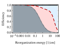
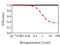
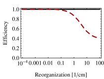
Figure 1: (Left panel) Efficiency $\eta$ (solid black) and contributions of initial state $\eta_{\rm init}$ (dash-dotted gray) and coherent evolution $\eta_{\rm init}+\eta_{\rm dyn}$ (dashed red) for a dimer that is based on the strongly coupled sites 1 and 2 of the Fenna-Matthews-Olson complex using the secular Redfield model. The initial state is at site 1 and the target is site 2. At a physiological value of around $\lambda=35/$cm, one finds $\eta_{\rm init}=0.0$ and $\eta_{\rm dyn}=0.43$. (Center panel) Efficiency and integrated coherence $\tilde{C}$ for the dimer with the secular Redfield approach. At $\lambda=35/$cm there is $\tilde{C}=0.37$. (Right panel) Same quantities as in the center panel for the dimer using the hierarchy equation of motion approach with 15 tiers of auxiliary systems. At $\lambda=35/$cm, one finds $\tilde{C}=0.44$. The parameters are $1/\kappa=1$ ps, $1/\Gamma=1$ ns, and $1/\gamma=50$ fs for all panels.

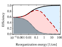
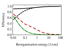
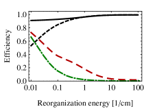
Figure 2: (Left panel) Efficiency $\eta$ (solid black) and contributions of initial state $\eta_{\rm init}$ (dash-dotted gray) and coherent evolution $\eta_{\rm init}+\eta_{\rm dyn}$ (dashed red) for the Fenna-Matthews-Olson complex using the secular Redfield model. The initial state is a classical mixture of site 1 and 6 and the target site for trapping is site 3. The actual system has a reorganization energy of around $\lambda=35/$cm, where $\eta_{\rm init}=0.0$ and $\eta_{\rm dyn}=0.17$. (Center panel) Efficiency for initial site 1 (solid black) and initial site 6 (dashed black) and integrated coherence $\tilde{C}$ for initial site 1 (dashed red) and initial site 6 (dash-dotted green) for the Fenna-Matthews-Olson complex with the secular Redfield approach. At $\lambda=35/$cm there is $\tilde{C}=0.0151$ (inital site 1) and $\tilde{C}=0.0017$ (initial site 6). (Right panel) Same quantities as in the center panel for the FMO complex using the scaled hierarchy equation of motion approach with four tiers of auxiliary systems. At $\lambda=35/$cm, one finds $\tilde{C}=0.020$ (inital site 1) and $\tilde{C}=0.0022$ (initial site 6). The parameters are $1/\kappa=1$ ps, $1/\Gamma=1$ ns, and $1/\gamma=50$ fs for all plots.

In Fig. 1, we present the two measures of coherence for a dimer system. For the dimer, we take the sites 1 and 2 of the FMO complex with $\epsilon_{1}=0/$cm, $\epsilon_{2}=120/$cm, and $J=-87.7/$cm, see Adolphs2006 , and room temperature. This system will also be the focus of the following sections on the atomistic detail simulations and quantum process tomography. Here, for studying the role of quantum coherence, we assume that the task is defined by the exciton initially being at the lower energy site 1 and the target site being site 2. In the left panel of Fig. 1 we show the efficiency $\eta$, the contribution $\eta_{\rm H}$ from Eq. (3), and $\eta_{\rm init}$ for the secular Redfield model. In the present small system, environment-assisted transport is relatively unimportant, with the efficiency as a function of the reorganziation energy being close to unity everywhere. The underlying contributions show a transition from a regime dominated by coherent evolution to a regime dominated by incoherent Lindblad jumps. At $\lambda=35/$cm, we find $\eta_{\rm init}=0\%$ and $\eta_{\rm H}=43\%$. In Fig. 1 (center panel), we find that the total coherence measure $\tilde{C}$ for the dimer is around $0.37$ for $\lambda=35/$cm. In Fig. 1 (right panel), the total coherence is plotted for the dimer in the hierarchy equation of motion approach. We use 15 tiers of auxiliary systems. At $\lambda=35/$cm, we find $\tilde{C}=0.44$; because of the sluggish, non-equilibrium bath there is more coherence than in the secular Redfield model.

In Fig. 2 (left panel), we present the coherent, decoherent, and initial state contribution to the ETE for the Fenna-Matthews-Olson complex as a function of the reorganization energy for the secular Redfield model at room temperature. We use the Hamiltonian given in Adolphs2006 and the contribution measures given in Equation (3) and by $\eta_{\rm init}$. The initial state is a classical mixture of site 1 and 6. For small reorganization energy, the efficiency is around $\eta=60$% and for larger reorganization energies we observe environment-assisted quantum transport (ENAQT)  Rebentrost2009b , with the efficiency rising up to almost $\eta=100$% for the physiological value of $\lambda=35/$cm. The contributions measures $\eta_{\rm dyn}$ and $\eta_{\rm init}$ reveal the underlying dynamics. The quantum dynamical contribution $\eta_{\rm dyn}$ is around $17$% at $\lambda=35/$cm . In our model, this part is due to an interplay of the Hamiltonian dynamics and the trapping/loss dynamics, which both have their preferred basis being the site basis. The main part of the efficiency at $\lambda=35/$cm is due to incoherent Lindblad jumps, having a value of $\eta_{\rm decoherence}=83$%. The initial state contribution is relevant only at small values of the reorganization energy.

In Fig. 2 (center and right panel), we compare the efficiency and the coherence measure $\tilde{C}$ for the secular Redfield and the hierarchy equation of motion approach Ishizaki2009 for the Fenna-Matthews-Olson complex. The initial state is either localized at site 1 or at site 6. Four tiers of auxiliary systems were used in the computation, which already lead to a good agreement with Ishizaki2009 for the dynamics at $\lambda=35$cm^-1, $1/\gamma=50$ fs, and room temperature. In Fig. 2 (right panel), ENAQT is observed with increasing reorganization energy also in the hierarchy approach, with the efficiency rising up to almost $\eta=100$% at $\lambda=35/$cm. In Fig. 2 (center and right panel), it is observed that the normalized total coherences of the density matrix decrease with increasing reorganization energy. For the secular Redfield case, we obtain $\tilde{C}(\lambda=35$cm${}^{-1})=0.0151$ for the initial site 1 and $\tilde{C}(\lambda=35$cm${}^{-1})=0.0017$ for the initial site 6. For the hierarchy case, we obtain more coherence, i.e. $\tilde{C}(\lambda=35$cm${}^{-1})=0.020$ for the initial site 1 and $\tilde{C}(\lambda=35$cm${}^{-1})=0.0022$ for the initial site 6. In both models, coherence is more important for the rugged energy landscape of the pathway from site 1 than for the funnel-type energy landscape of the pathway from site 6.

Master equation approaches, such as the ones discussed in this section suffer from various drawbacks. Redfield theory is only applicable in the limit of weak system bath coupling and does not take into account non-equilibrium molecular reorganization effects. The hierarchy equation of motion approach assumes Gaussian fluctuations and Ohmic Drude-Lorentz spectral densities. The detailed atomistic structure of the protein and the chlorophylls is not taken into account in these approaches. The results thus provide a general indication of the behavior of the actual system but not a conclusive and detailed theoretical proof. In the next section, we will present a first step toward such a detailed study with our combined molecular dynamics/quantum chemistry method. The atomistic structure is included and realistic spectral densities can be obtained. We also present a straightforward method to simulate exciton dynamics beyond master equations. We thus address the second question of the microscopic origins of the long-lived quantum coherence.

III Molecular Dynamics Simulations

Among many other biologically functional components, protein complexes are essential components of the photosynthetic system. Proteins remain as one of the main topics of biophysical research due to their diverse and unidentified structure-function relationship. Many biological units are highly optimized and efficient, so that even a point mutation of a single amino acid in conserved region often results in the loss of the functionality.  Tamoi2010 ; Jahns2002 ; Pesaresi1997 Have the photosynthetic system adopted quantum mechanics to improve its efficiency in its course of evolution? To answer this question, careful characterization of the protein environment to the atomistic detail is necessary to identify the microscopic origin of the long-lived quantum coherence. As explained in the previous section, the contribution of the quantum coherence to the energy transfer efficiency in biological systems have been successfully carried out, yet a more detailed description of the bath in atomic detail would be desirable to investigate the structure-function relationship of the protein complex and to test validity of the assumptions used in popular models of the photosynthetic system.

The site energy of a chromophore is a complex function of the configuration of the chromophore molecule, and the relative orientation of the molecule to that of the embedding protein and that of other chromophore molecules. Factors affecting site energies have intractably large degrees of freedom, so it is reasonable to treat those degrees of freedom as the bath of an open quantum system. The state of the system is assumed to be restricted to the single exciton manifold. To construct a system-bath relationship with atomistic detail of the bath, we start from the total Hamiltonian operator, and decomposed the operator in such a way that the system-bath Hamiltonian is not assumed to be any specific functional form:

$$\begin{split}{H}_{total}&=\sum_{m}\epsilon_{m}(\bm{R}_{ch},\bm{R}_{prot})|m\rangle\langle m|+\sum_{m,n}\left\{J_{mn}(\bm{R}_{ch},\bm{R}_{prot})|m\rangle\langle n|+c.c.\right\}\\ &\quad+{T}_{ch}+{T}_{prot}+{V}_{ch}(\bm{\sigma},\bm{R}_{ch},\bm{R}_{prot})+{V}_{prot}(\bm{R}_{ch},\bm{R}_{prot}).\end{split}$$ (5)

$\epsilon_{m}$ represents the site energy of $m$th site, $J_{mn}$ is the coupling constant between $m$th and $n$th sites. $\bm{\sigma}$ denotes the excitonic state of chromophores, $\bm{R}_{ch}$ corresponds to the nuclear coordinates of chromophore molecules, and $\bm{R}_{prot}$ are the nuclear coordinates of the remaining protein and enclosing water molecules. ${T}$ and ${V}$ are the corresponding kinetic and potential energy operators for the chromophores and proteins respectively under Born-Oppenheimer approximation. The potential energy term for chromophores depends on the exciton state of the systen, because dynamics of a molecule will be governed by different Born-Oppenheimer surface when its excitonic state changes. However, as a first approximation, we assumed that the change of Born-Oppenheimer surfaces does not affect the bath dynamics significantly. With this assumption, we can ignore the dependence of the excitonic state in the $V_{ch}$ term and the system-bath Hamiltonian only contains the one way influence from the bath to the system:

$$\begin{split}{H}_{total}&\approx\sum_{m}\epsilon_{m}(\bm{R}_{ch},\bm{R}_{prot})|m\rangle\langle m|+\sum_{m,n}\left\{J_{mn}(\bm{R}_{ch},\bm{R}_{prot})|m\rangle\langle n|+c.c.\right\}\\ &\quad+\sum_{m}\epsilon_{m}(\bm{R}_{ch},\bm{R}_{prot})|m\rangle\langle m|+{T}_{ch}+{T}_{prot}+{V}_{ch}(\bm{R}_{ch},\bm{R}_{prot})+{V}_{prot}(\bm{R}_{ch},\bm{R}_{prot})\\ &=\underbrace{\sum_{m}\bar{\epsilon}_{m}|m\rangle\langle m|+\sum_{m,n}\left\{\bar{J}_{mn}|m\rangle\langle n|+c.c.\right\}}_{{H}_{S}}\\ &\quad+\underbrace{\sum_{m}\left\{\epsilon_{m}(\bm{R}_{ch},\bm{R}_{prot})-\bar{\epsilon}_{m}\right\}|m\rangle\langle m|+\left[\sum_{m,n}\left\{J_{mn}(\bm{R}_{ch},\bm{R}_{prot})-\bar{J}_{mn}\right\}|m\rangle\langle n|+c.c.\right]}_{{H}_{SB}}\\ &\quad+\underbrace{{T}_{ch}+{T}_{prot}+{V}_{ch}(\bm{R}_{ch},\bm{R}_{prot})+{V}_{prot}(\bm{R}_{ch},\bm{R}_{prot})}_{{H}_{B}}.\end{split}$$ (6)

Based on this decomposition of the total Hamiltonian, we set up a model of the FMO complex in atomistic detail with the AMBER force field Cornell1995 ; Ceccarelli2003 and approximate the propagation of the entire complex by classical mechanics. Molecular dynamics simulations were conducted at 77K and 300K with an isothermal-isobaric (NPT) ensemble. The parameters for the system and the system-bath Hamiltonian were calculated using quantum chemistry methods along the trajectory from the molecular dynamics simulation. $\epsilon_{m}$ was calculated using the Q-Chem quantum chemistry package. Shao2006 The electronic excitations were modeled using the time-dependent density functional theory using the Tamm-Dancoff approximation. The density functional employed was BLYP and the basis set employed was 3-21G*. External charges from the force field were included in the calculation as the electrostatic external potential. The coupling terms, $J_{mn}$, were obtained from the Hamiltonian presented in  Adolphs2006 and considered to be constant in time. $\bar{\epsilon}_{m}$ was chosen as time averaged site energy for the $m$th site to minimize the magnitude of the system-bath Hamiltonian. In this work, only site 1 and site 2 were considered for the exciton dynamics. However, the methodology can be applied for the exciton dynamic of all seven chromophores.

To obtain a closed-form equation for the reduced density matrix, we applied mean-field approximation May2004 ; because no feedback from the system to the bath was assumed, the state of the bath is not affected by the state of the system. Therefore, the total density matrix, $W(t)$, can be factorized into the reduced density matrix $\rho(t)$, and $B(t)$ which is defined only in the Hilbert space of the bath. With additional assumption that the bath is in thermal equilibrium, we can obtain the closed equation for the reduced density matrix.

$$\begin{split}\frac{\partial}{\partial t}\rho(t)&=-\frac{i}{\hbar}\left[{H}_{S},\rho(t)\right]-\frac{i}{\hbar}{\rm Tr}\left\{\left[{H}_{SB},W(t)\right]\right\}\\ &\approx-\frac{i}{\hbar}\left[{H}_{S},\rho(t)\right]-\frac{i}{\hbar}\left[{\rm Tr}\left\{{H}_{SB}B(t)\right\},\rho(t)\right]\\ &\approx-\frac{i}{\hbar}\left[{H}_{S},\rho(t)\right]-\frac{i}{\hbar}\left[{\rm Tr}\left\{{H}_{SB}B_{eq}(t)\right\},\rho(t)\right].\end{split}$$ (7)

Thermal equilibrium of the bath was ensured by the thermostat of the molecular dynamics simulation. Thus, the reduced density matrix was obtained by Monte Carlo integration of 4000 independent instances of unitary quantum evolution with respect to the thermally equilibrated bath. Each instance was propagated by integrating the Schrödinger equation with the simple exponential integrator.

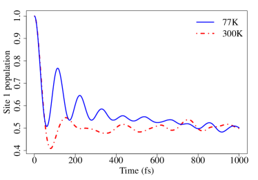
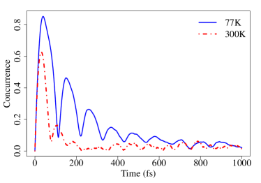
Figure 3: (Left panel) Time evolution of the exciton population at the site 1 ($\rho_{11}$) based on the strongly coupled site 1 and 2 of the FMO complex at 77K and 300K. The initial pure state $\rho=|1\rangle\langle 1|$ was propagated using Monte Carlo integration of unitary evolutions, where the time-dependent site energies are obtained from a combined molecular dyanmics/quantum chemistry approach. The asymptotic distribution does not follow a Boltzmann distribution because relaxation of the system to the bath is not considered. (Right panel) The concurrence between site 1 and 2 at 77K and 300K. Quantum coherence lives longer at a lower temperature.

Figure 3 shows the change of the population of the site 1, $\rho_{11}$, and the concurrence between site 1 and 2. The population is evenly distributed between the two sites because relaxation was not considered. The concurrence, $2|\rho_{12}|$, is an indicator of pairwise entanglement for the system. Sarovar2010 Note that the coherence builds up during the first $\approx$ 100 fs , and then decreases subsequently due to the decoherence from the bath.

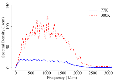
Figure 4: (Left panel) Spectral density from the autocorrelation function of the site 1 of the FMO complex from the molecular dynamics simulation at 77K and 300K. While the spectral density reflects the characteristic vibrational modes of the protein and the chromophore molecule, high-frequency modes are overpopulated due to the limitation of the Newtonian mechanics. (Right panel) Absorption spectrum of site 1 and 2 at 77K and 300K.

Figure 4 shows the spectral density of the first chromophore. Although the spectral density of the bath from molecular dynamics simulation shows characteristic frequencies related to the actual protein environment and the bacteriochloropyll molecule, high-frequency modes are overpopulated due to the limitation of the classical mechanics. There are efforts to incorporate quantum effects into the classical molecular dynamics simulation in a slightly different context, Egorov1999 ; Skinner2001 ; Stock2009 and we are investigating the possibilities of applying these corrections.

Another simplification employed was the omission of the feedback from exciton states. When the exciton state of a bacteriochlorophyll is changed, the Born-Oppenheimer surface which governs the dynamics of the chromophore molecule should be also changed. The current scheme only propagates the protein complex on the electronically ground-state surface. Incorporating the feedback could lead to the different characteristics of the protein bath. There exist several schemes for mixed quantum-classical dynamics Tully1990 ; Ben-Nun2000 ; Wu2005 which potentially resolve the problem at the additional computational cost of simultaneously propagating excitons and protein bath.

Calculations are underway to carry out the full seven-site simulation of the FMO complex at different temperatures to compare with experimental temperature-dependent results Panitchayangkoon2010 .

In the following final section, we will describe our quantum process tomography scheme, which is a spectroscopic technique associated with a computational procedure for direct extraction of the parameters related to the quantum evolution of the system, in terms of quantum process maps.

IV Quantum Process Tomography

So far, we have delved into several theoretical models to characterize quantum coherence in the entire FMO complex and in a dimer subsystem of it. Experimentally, however, a clear characterization of this coherence is still elusive. Signatures of long lived quantum superpositions between excitonic states in multichromophoric systems are potentially monitored through four wave-mixing techniques Engel2007 ; cheng ; mukamel . However, a transparent description of the evolving quantum state of the probed system is not necessarily obtained from a single realization of such experiments. In these, a series of three weak incoming ultrashort pulses sent from a noncollinear setup induce a macroscopic third order polarization in the sample. The latter manifests in a time dependent spatial grating through which a fourth pulse diffracts. From an operational standpoint, this last pulse selects the spatial Fourier component of the polarization which corresponds to its wavevector (heterodyne detection), hence earning the name of four wave-mixing for this technique (FWM) mukamel . Extracting specific Fourier components of the induced polarization allows for the selection of a particular set of processes in the density matrix of the probed system, as each wavevector is associated with a carrier frequency of the pulse. These processes can be intuitively understood by keeping track of the dual Feynman diagrams that account for the perturbations that the pulses induce on the bra or ket sides of the density matrix of the probed system. Whereas the analysis of these experiments is naturally carried out in the density matrix formalism, an important question is whether the density matrix itself can be imaged via these experiments, a problem known as quantum state tomography (QST) nielsenchuang . If this were possible, quantum process tomography (QPT) could also be carried out, therefore providing a complete characterization of excited state dynamics cirac . In a previous study, we showed that a series of two-color heterodyned rephasing photon-echo (PE) experiments repeated in different polarization configurations yields the necessary information to carry out QST and QPT of the single-exciton manifold of a coupled heterodimer YuenMohseni . In the present article, we adapt our previous theory to extract this information from two-dimensional spectra, similar to those employed in current experiments.

We begin by reviewing some basic aspects of QPT. Under very general assumptions, the evolution of an open quantum system can be described by a linear transformation sudarshan :

$$\rho_{ab}(T)=\sum_{cd}\chi_{abcd}(T)\rho_{cd}(0),$$ (8)

where $\rho_{ab}(T)$ is the element $ab$ of the reduced density matrix $\rho$ of the system at time $T$. Equation (8) is remarkable in that $\chi(T)$ is independent of the initial state. Knowledge of $\chi(T)$ implies a complete characterization of the dynamics of the reduced system and, in fact, QPT can be operationally defined as the procedure to obtain $\chi(T)$. Conceptually, it is straightforward to recognize that, due to linearity, $\chi(T)$ can be inverted by preparing a complete set of inputs, evolving them for time $T$, and detecting the outputs along a complete basis. In the context of nonlinear optical spectroscopy, this is exactly the strategy we shall follow, with a few caveats due to experimental constraints.

To place the discussion in context, we shall be again concerned with the subsystem composed of the excitonic dimer between sites 1 and 2 of the FMO complex. For simplicity, we ignore the rest of the sites in this theoretical study. We only need to be concerned with four eigenstates of this model system: The ground state $|g\rangle$, the delocalized single-excitons $|\alpha\rangle$ and $|\beta\rangle$, and the biexciton $|f\rangle$, which in the photosynthetic system can be safely assumed to be the direct sum of the single-excitons without significant interactions between them. Therefore, the biexciton energy level is just $\omega_{f}=\omega_{\alpha}+\omega_{\beta}$. We label the delocalized excitons so that $|\alpha\rangle$ is the higher energy eigenstate compared to $|\beta\rangle$. Denoting the transition energies between the $i$-th and the $j$-th states by $\omega_{ij}=\omega_{i}-\omega_{j}$, it follows that $\omega_{\alpha g}=\omega_{f\beta}$ and $\omega_{\beta g}=\omega_{f\alpha}$ minhaengbook . The excitonic system is not isolated, and in fact, it interacts with a phonon and photon bath which induces relaxation and dephasing processes in it.

The experimental technique we consider is photon-echo (PE) spectroscopy, which is a particular subset of FWM techniques where the wavevector of the fourth pulse corresponds to the phase-matching condition $\bm{k}_{PE}=-\bm{k_{1}}+\bm{k_{2}}+\bm{k_{3}}$, with $\bm{k}_{i}$ being the wavevector corresponding to the $i$-th pulse. Here, the labeling of the pulses corresponds to the order in which the fields interact with the sample. Typically, the ultrashort pulses employed to study these excitonic systems possess an optical carrier frequency, therefore allowing transitions which are resonant with the frequency components $\pm\omega_{\beta g}$ and $\pm\omega_{\alpha g}$. In PE experiments, the first pulse centered at $t_{1}$ creates an optical coherence beating at a frequency $\omega_{g\alpha}$ or $\omega_{g\beta}$. At $t_{2}=t_{1}+\tau$, the second pulse creates a coherence or a population in the single exciton manifold. At $t_{3}=t_{2}+T$, the third pulse generates another optical coherence, but this time, beating at the frequencies opposite to the ones in the first interval, that is, at frequencies $\omega_{\alpha g}$ or $\omega_{\beta g}$, causing a rephasing echo of the signal. The heterodyne detection of the nonlinear polarization signal $P_{PE}(\tau,T,t)$ occurs at time $t_{4}=t_{3}+t$. Borrowing from NMR jargon, the intervals $(t_{1},t_{2})$, $(t_{2},t_{3})$, and $(t_{3},t_{4})$ are traditionally refered to as coherence, waiting, and echo times, and their durations are $\tau$, $T$, and $t$, respectively. This nomenclature should not be taken literally. For example, in most case, coherences do not only evolve in the coherence time, but in the waiting and echo times. Similarly, the waiting time is often referred to as population time, which hosts dynamics of both populations and coherences. For a historical perspective on this vocabulary, we refer the reader to any comprehensive NMR treatise such as goldmanbook .

The experiment is systematically repeated for many durations for each interval. In order to ’watch’ single-exciton dynamics, it is convenient to isolate the changes on the signal due to the waiting time $T$. This exercise is accomplished by performing a double Fourier transform of the signal along the $\tau$ and $t$ axes, which yields a 2D spectra that evolves in $T$ ginsberg ; jonas ; minhaeng :

$$S(\omega_{\tau},T,\omega_{T})=\int_{0}^{\infty}d\tau\int_{0}^{\infty}dtP_{PE}(\tau,T,t)e^{-i\omega_{\tau}\tau+i\omega_{T}T}$$ (9)

In order to map a PE experiment to a QPT, we identify the coherence interval as the preparation step and the echo interval as the detection step. This assumption implies that the optical coherence intervals have well characterized dynamics. This hypothesis is reasonable due to a separation of timescales where optical coherences will presumably decay exponentially due to pure dephasing and not due to intricate phonon-induced processes. Therefore, the 2D spectrum consists of four Lorentzian peaks centered about $(\omega_{\tau},\omega_{t})=(\omega_{\alpha g},\omega_{\alpha g}),(\omega_{\alpha g},\omega_{\beta g}),(\omega_{\beta g},\omega_{\alpha g}),(\omega_{\beta g},\omega_{\beta g})$. In this discussion, we shall ignore inhomogeneous broadening, noting that it can always be accounted for as a convolution of the signal with the distrubtion of inhomogeneity. The width of these Lorentzians can be directly related to the dephasing rates of the optical coherences. Loosely speaking, a particular value on the $\omega_{\tau}$ axis of the spectrum indicates a specific type of state preparation, whereas the $\omega_{t}$ axis is related to a particular detection. More precisely, a peak in the 2D spectrum displays the correlations between the frequency beats from the coherence and echo intervals. A crucial realization is that the amplitude of these peaks can be written as a linear combination of elements of the time evolving excitonic density matrix stemming from different initial states, that is, of elements of $\chi(T)$ itself YuenMohseni :

$$\tilde{S}(\omega_{\alpha g},T,\omega_{\alpha g}) = -C_{\omega_{1}}^{\alpha}C_{\omega_{2}}^{\alpha}(\bm{\mu}_{\alpha g}\cdot\bm{e}_{1})(\bm{\mu}_{\alpha g}\cdot\bm{e}_{2})$$ (10)

$$\times\{C_{\omega_{3}}^{\alpha}[(\bm{\mu}_{\alpha g}\cdot\bm{e}_{3})(\bm{\mu}_{\alpha g}\cdot\bm{e}_{4})(\chi_{gg\alpha\alpha}(T)-1-\chi_{\alpha\alpha\alpha\alpha}(T))$$

$$+(\bm{\mu}_{f\beta}\cdot\bm{e}_{3})(\bm{\mu}_{f\beta}\cdot\bm{e}_{4})\chi_{\beta\beta\alpha\alpha}(T)]$$

$$+C_{\omega_{3}}^{\beta}[(\bm{\mu}_{f\alpha}\cdot\bm{e}_{3})(\bm{\mu}_{f\beta}\cdot\bm{e}_{4})-(\bm{\mu}_{\beta g}\cdot\bm{e}_{3})(\bm{\mu}_{\alpha g}\cdot\bm{e}_{4}))\chi_{\alpha\beta\alpha\alpha}(T)]\}$$

$$-C_{\omega_{1}}^{\alpha}C_{\omega_{2}}^{\beta}(\bm{\mu}_{\alpha g}\cdot\bm{e}_{1})(\bm{\mu}_{\beta g}\cdot\bm{e}_{2})$$

$$\times\{C_{\omega_{3}}^{\alpha}[(\bm{\mu}_{\alpha g}\cdot\bm{e}_{3})(\bm{\mu}_{\alpha g}\cdot\bm{e}_{4})(\chi_{gg\beta\alpha}(T)-\chi_{\alpha\alpha\beta\alpha}(T))$$

$$+(\bm{\mu}_{f\beta}\cdot\bm{e}_{3})(\bm{\mu}_{f\beta}\cdot\bm{e}_{4})\chi_{\beta\beta\beta\alpha}(T)]$$

$$+C_{\omega_{3}}^{\beta}[((\bm{\mu}_{f\alpha}\cdot\bm{e}_{3})(\bm{\mu}_{f\beta}\cdot\bm{e}_{4})-(\bm{\mu}_{\beta g}\cdot\bm{e}_{3})(\bm{\mu}_{\alpha g}\cdot\bm{e}_{4}))\chi_{\alpha\beta\beta\alpha}(T)]\},$$

$$\tilde{S}(\omega_{\alpha g},T,\omega_{\beta g}) = -C_{\omega_{1}}^{\alpha}C_{\omega_{2}}^{\alpha}(\bm{\mu}_{\alpha g}\cdot\bm{e}_{1})(\bm{\mu}_{\alpha g}\cdot\bm{e}_{2})$$ (11)

$$\times\{C_{\omega_{3}}^{\beta}[(\bm{\mu}_{\beta g}\cdot\bm{e}_{3})(\bm{\mu}_{\beta g}\cdot\bm{e}_{4})(\chi_{gg\alpha\alpha}(T)-1-\chi_{\beta\beta\alpha\alpha}(T))$$

$$+(\bm{\mu}_{f\alpha}\cdot\bm{e}_{3})(\bm{\mu}_{f\alpha}\cdot\bm{e}_{4})\chi_{\alpha\alpha\alpha\alpha}(T)]$$

$$+C_{\omega_{3}}^{\alpha}[((\bm{\mu}_{f\beta}\cdot\bm{e}_{3})(\bm{\mu}_{f\alpha}\cdot\bm{e}_{4})-(\bm{\mu}_{\alpha g}\cdot\bm{e}_{3})(\bm{\mu}_{\beta g}\cdot\bm{e}_{4}))\chi_{\beta\alpha\alpha\alpha}(T)]\}$$

$$-C_{\omega_{1}}^{\alpha}C_{\omega_{2}}^{\beta}(\bm{\mu}_{\alpha g}\cdot\bm{e}_{1})(\bm{\mu}_{\beta g}\cdot\bm{e}_{2})$$

$$\times\{C_{\omega_{3}}^{\beta}[(\bm{\mu}_{\beta g}\cdot\bm{e}_{3})(\bm{\mu}_{\beta g}\cdot\bm{e}_{4})(\chi_{gg\beta\alpha}(T)-\chi_{\beta\beta\beta\alpha}(T))$$

$$+(\bm{\mu}_{f\alpha}\cdot\bm{e}_{3})(\bm{\mu}_{f\alpha}\cdot\bm{e}_{4})\chi_{\alpha\alpha\beta\alpha}(T)]$$

$$+C_{\omega_{3}}^{\alpha}[((\bm{\mu}_{f\beta}\cdot\bm{e}_{3})(\bm{\mu}_{f\alpha}\cdot\bm{e}_{4})-(\bm{\mu}_{\alpha g}\cdot\bm{e}_{3})(\bm{\mu}_{\beta g}\cdot\bm{e}_{4}))\chi_{\beta\alpha\beta\alpha}(T)]\},$$

$$\tilde{S}(\omega_{\beta g},T,\omega_{\alpha g}) = -C_{\omega_{1}}^{\beta}C_{\omega_{2}}^{\beta}(\bm{\mu}_{\beta g}\cdot\bm{e}_{1})(\bm{\mu}_{\beta g}\cdot\bm{e}_{2})$$ (12)

$$\times\{C_{\omega_{3}}^{\alpha}[(\bm{\mu}_{\alpha g}\cdot\bm{e}_{3})(\bm{\mu}_{\alpha g}\cdot\bm{e}_{4})(\chi_{gg\beta\beta}(T)-1-\chi_{\alpha\alpha\beta\beta}(T))$$

$$+(\bm{\mu}_{f\beta}\cdot\bm{e}_{3})(\bm{\mu}_{f\beta}\cdot\bm{e}_{4})\chi_{\beta\beta\beta\beta}(T)]$$

$$+C_{\omega_{3}}^{\beta}[(\bm{\mu}_{f\alpha}\cdot\bm{e}_{3})(\bm{\mu}_{f\beta}\cdot\bm{e}_{4})-(\bm{\mu}_{\beta g}\cdot\bm{e}_{3})(\bm{\mu}_{\alpha g}\cdot\bm{e}_{4}))\chi_{\alpha\beta\beta\beta}(T)]\}$$

$$-C_{\omega_{1}}^{\beta}C_{\omega_{2}}^{\alpha}(\bm{\mu}_{\beta g}\cdot\bm{e}_{1})(\bm{\mu}_{\alpha g}\cdot\bm{e}_{2})$$

$$\times\{C_{\omega_{3}}^{\alpha}[(\bm{\mu}_{\alpha g}\cdot\bm{e}_{3})(\bm{\mu}_{\alpha g}\cdot\bm{e}_{4})(\chi_{gg\alpha\beta}(T)-\chi_{\alpha\alpha\alpha\beta}(T))$$

$$+(\bm{\mu}_{f\beta}\cdot\bm{e}_{3})(\bm{\mu}_{f\beta}\cdot\bm{e}_{4})\chi_{\beta\beta\alpha\beta}(T)]$$

$$+C_{\omega_{3}}^{\beta}[((\bm{\mu}_{f\alpha}\cdot\bm{e}_{3})(\bm{\mu}_{f\beta}\cdot\bm{e}_{4})-(\bm{\mu}_{\beta g}\cdot\bm{e}_{3})(\bm{\mu}_{\alpha g}\cdot\bm{e}_{4}))\chi_{\alpha\beta\alpha\beta}(T)]\},$$

$$\tilde{S}(\omega_{\beta g},T,\omega_{\beta g}) = -C_{\omega_{1}}^{\beta}C_{\omega_{2}}^{\beta}(\bm{\mu}_{\beta g}\cdot\bm{e}_{1})(\bm{\mu}_{\beta g}\cdot\bm{e}_{2})$$ (13)

$$\times\{C_{\omega_{3}}^{\beta}[(\bm{\mu}_{\beta g}\cdot\bm{e}_{3})(\bm{\mu}_{\beta g}\cdot\bm{e}_{4})(\chi_{gg\beta\beta}(T)-1-\chi_{\beta\beta\beta\beta}(T))$$

$$+(\bm{\mu}_{f\alpha}\cdot\bm{e}_{3})(\bm{\mu}_{f\alpha}\cdot\bm{e}_{4})\chi_{\alpha\alpha\beta\beta}(T)]$$

$$+C_{\omega_{3}}^{\alpha}[((\bm{\mu}_{f\beta}\cdot\bm{e}_{3})(\bm{\mu}_{f\alpha}\cdot\bm{e}_{4})-(\bm{\mu}_{\alpha g}\cdot\bm{e}_{3})(\bm{\mu}_{\beta g}\cdot\bm{e}_{4}))\chi_{\beta\alpha\beta\beta}(T)]\}$$

$$-C_{\omega_{1}}^{\beta}C_{\omega_{2}}^{\alpha}(\bm{\mu}_{\beta g}\cdot\bm{e}_{1})(\bm{\mu}_{\alpha g}\cdot\bm{e}_{2})$$

$$\times\{C_{\omega_{3}}^{\beta}[(\bm{\mu}_{\beta g}\cdot\bm{e}_{3})(\bm{\mu}_{\beta g}\cdot\bm{e}_{4})(\chi_{gg\alpha\beta}(T)-\chi_{\beta\beta\alpha\beta}(T))$$

$$+(\bm{\mu}_{f\alpha}\cdot\bm{e}_{3})(\bm{\mu}_{f\alpha}\cdot\bm{e}_{4})\chi_{\alpha\alpha\alpha\beta}(T)]$$

$$+C_{\omega_{3}}^{\alpha}[((\bm{\mu}_{f\beta}\cdot\bm{e}_{3})(\bm{\mu}_{f\alpha}\cdot\bm{e}_{4})-(\bm{\mu}_{\alpha g}\cdot\bm{e}_{3})(\bm{\mu}_{\beta g}\cdot\bm{e}_{4}))\chi_{\beta\alpha\alpha\beta}(T)]\}.$$

Here, the expressions have been obtained using the rotating-wave approximation, as well as the assumption of no overlap between pulses. $\bm{\mu}_{pq}=\bm{\mu}_{qp}$ is the transition dipole moment between states $p,q\in\{g,\alpha,\beta,f\}$. We have rescaled the spectra amplitudes to eliminate the details of the lineshape by multiplying them by the dephasing rates of the optical coherences in the coherence and echo intervals,

$$\tilde{S}(\omega_{pg},T,\omega_{qg})=\Gamma_{gp}\Gamma_{qg}S(\omega_{pg},T,\omega_{qg}).$$ (14)

The coefficient $C_{\omega_{i}}^{p}$ is the amplitude of the $i$-th pulse at the frequency $\omega_{pg}$,

$$C_{\omega_{i}}^{p}=-\frac{\Lambda}{i}\sqrt{2\pi\sigma^{2}}e^{-\sigma^{2}(\omega_{pg}-\omega_{i})^{2}/2},$$ (15)

with $\Lambda$ being the strength of the pulse and $\sigma$ the width of the Gaussian pulse in time domain. Also, $\bm{e}_{i}$ is the polarization of the $i$-th pulse. Both $C_{\omega_{i}}^{p}$ and $\bm{e}_{i}$ are experimentally tunable parameters for the pulses.

Whereas Equations (14) and (15) presented in YuenMohseni correspond to a single value of $\tau$ and $t$, Equations (10), (11), (12), and (13) stem from Fourier transform of data collected at many $\tau$ and $t$ times. Therefore, in principle, a 2D spectrum provides a more robust source of information from which to invert $\chi(T)$ than in the suggested 1D experiment. The displayed equations, albeit lengthy, are easy to interpret. For instance, consider the term which is proportional to $\chi_{\alpha\beta\alpha\alpha}(T)$ in Equation (10), which stems from the Feynman diagram depicted in Fig. 5. As expected, it consists of a waiting time where the initially prepared population $|\alpha\rangle\langle\alpha|$ is transferred to the coherence $|\alpha\rangle\langle\beta|$. This waiting time is escorted by a coherence $|g\rangle\langle\alpha|$ oscillating as $e^{(-i\omega_{g\alpha}-\Gamma_{g\alpha})\tau}$ which evolves during the coherence time and another set of coherences $|f\rangle\langle\beta|$ and $|\alpha\rangle\langle g|$ which evolve during the echo time as $e^{(-i\omega_{f\beta}-\Gamma_{f\beta})t}=e^{(-i\omega_{\alpha g}-\Gamma_{\alpha g})t}$. These two intervals correspond to the diagonal peak located at $(\omega_{\alpha g},\omega_{\alpha g})$. Other processes that exhibit oscillations at those two respective frequencies appear as additional terms in the equation corresponding to that particular peak.

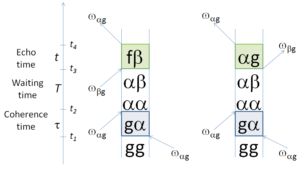
Figure 5: Dual Feynman diagrams that account for the population to coherence transfer terms $\chi_{\alpha\beta\alpha\alpha}(T)$ in quantum process tomography.

In Ref. YuenMohseni , we showed that there are sixteen real valued parameters of $\chi(T)$ which need to be determined at every value of $T$ in order to carry out QPT of the single exciton manifold of a heterodimer. For an illustration, we shall describe how to obtain the elements $\chi_{ij\alpha\alpha}(T)$. These quantities are shown in Fig. 6 and have been computed using the Ishizaki-Fleming model, with a bath correlation of 150 $fs$ Ishizaki2009 . They display rich and nontrivial phonon-induced behavior, such as the spontaneous generation of coherence from a population in an eigenstate of the excitonic Hamiltonian, and therefore, is a very good example of how QPT provides access to this nontrivial information via the repetition of a series of 2D PE experiments. For this particular set of $\chi(T)$ elements, we shall exploit the waveform of the pulses but not their polarizations, and for simplicitly we will assume the polarization configuration $xxxx$ for each of the pulses including the heterodyning.

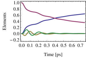
Figure 6: Transfer of population in eigenstate $|\alpha\rangle\langle\alpha|$ to other populations and coherences in the eigenbasis of the single exciton Hamiltonian. The hierarchy equation of motion approach is used for a dimer system based on the parameters of the site 1 and site 2 subsystem of the Fenna-Matthews-Olson complex. Population in $|\alpha\rangle\langle\alpha|$ decreases ($\chi_{\alpha\alpha\alpha\alpha}(T)$, purple) and is transferred to $|\beta\rangle\langle\beta|$ ($\chi_{\beta\beta\alpha\alpha}(T)$, blue). Emergence of coherence from the initial population occurs in this model ($\Re\{\chi_{\alpha\beta\alpha\alpha}(T)\}$, yellow and $\Im\{\chi_{\alpha\alpha\alpha\alpha}(T)\}$, green).

Consider the possibility of using pulses with carrier frequencies centered about $\omega_{\alpha g}$ and $\omega_{\beta g}$ respectively, and such that their bandwidth is narrow enough that the pulse centered about $\omega_{\alpha g}$ has negligible component at $\omega_{\beta g}$ and vice versa. Then, we can carry out an experiment such that $\frac{|C_{\omega_{1}}^{\alpha}|}{|C_{\omega_{1}}^{\beta}|},\frac{|C_{\omega_{2}}^{\alpha}|}{|C_{\omega_{2}}^{\beta}|},\frac{|C_{\omega_{3}}^{\beta}|}{|C_{\omega_{3}}^{\alpha}|}\gg 1$ (experiment 1) for all $i$ and notice that the diagonal peak at $(\omega_{\alpha g},\omega_{\alpha g})$ reduces to:

$$\langle\tilde{S}(\omega_{\alpha},T,\omega_{\alpha})\rangle_{xxxx}=-C_{\omega_{1}}^{\alpha}C_{\omega_{2}}^{\alpha}C_{\omega_{3}}^{\beta} \langle(\bm{\mu}_{\alpha g}\cdot\bm{e}_{1})(\bm{\mu}_{\alpha g}\cdot\bm{e}_{2})[(\bm{\mu}_{f\alpha}\cdot\bm{e}_{3})(\bm{\mu}_{f\beta}\cdot\bm{e}_{4})$$

$$-(\bm{\mu}_{\beta g}\cdot\bm{e}_{3})(\bm{\mu}_{\alpha g}\cdot\bm{e}_{4}))]\rangle_{xxxx}\chi_{\alpha\beta\alpha\alpha}(T)$$

which implies that its evolution with respect to $T$ directly monitors the transfer of the population prepared at $|\alpha\rangle\langle\alpha|$ to the coherence at $|\alpha\rangle\langle\beta|$. Here, $\langle\cdot\rangle_{xxxx}$ denotes an isotropic average of the experiments performed with the $xxxx$ polarization configuration. $\chi_{\alpha\beta\alpha\alpha}(T)$ can be directly obtained if information of the dipole moments is known in advance. As can be checked easily, $\chi_{\alpha\beta\alpha\alpha}(T)=(\chi_{\beta\alpha\alpha\alpha}(T))^{*}$ can, in principle, be also obtained directly from an experiment where $\frac{|C_{\omega_{i}}^{\alpha}|}{|C_{\omega_{i}}^{\beta}|}\gg 1$ for all $i$ (experiment 2) and monitoring $\langle\tilde{S}(\omega_{\alpha},T,\omega_{\beta})\rangle_{xxxx}$. Redundant measurements can be used as ways of effectively constraining the QPT.

Similarly, the transfer from $|\alpha\rangle\langle\alpha|$ to other populations can be extracted by monitoring $\langle\tilde{S}(\omega_{\alpha},T,\omega_{\alpha})\rangle_{xxxx}$ in experiment 2 and $\langle\tilde{S}(\omega_{\alpha},T,\omega_{\beta})\rangle_{xxxx}$ in experiment 1. These two linearly independent conditions are enough to extract $\chi_{gg\alpha\alpha}(T)$, $\chi_{\alpha\alpha\alpha\alpha}(T)$, and $\chi_{\beta\beta\alpha\alpha}(T)$, since there is a third independent condition based on trace preservation which reads $\chi_{gg\alpha\alpha}(T)+\chi_{\alpha\alpha\alpha\alpha}(T)+\chi_{\beta\beta\alpha\alpha}(T)=1$.

It is now important to verify whether the suggested experiments are feasible. In order to ensure conditions of the form $\frac{|C_{\omega_{i}}^{\alpha}|}{|C_{\omega_{i}}^{\beta}|}\gg 1$, we need $\sigma\sim\frac{3}{\omega_{\alpha g}-\omega_{\beta g}}\sim 470$ fs, that is, the pulse needs to be long enough to guarantee the narrow band condition. This requirement, although attractive from a pedagogical standpoint since it yields block diagonal sets of linear equations, is a nuisance from a practical perspective, as decoherence mechanisms might be in the same timescale and might not be ’seen’ with such long pulses. However, the only essential requirement is a toolbox of two different waveforms for the pulses. A more sensible choice is a set of pulses centered about $\omega_{\alpha g}$ and $\omega_{\beta g}$ respectively, but having $\sigma\sim 100$ fs. By carrying out 8 experiments alternating the two waveforms in each of the three pulses, each of the terms in Equations (10), (11), (12), and (13) which are proportional to $C_{\omega_{1}}^{i}C_{\omega_{2}}^{j}C_{\omega_{3}}^{k}$ for $i,j,k\in\{\alpha,\beta\}$ may be inverted to yield the block diagonal set of equations discussed above.

In summary, we have presented three different tools for unraveling the role of quantum coherence in biological systems: a) techniques for obtaining the contribution of quantum coherences to biological processes; b) a microscopic simulation approach to explore the dynamics of these systems by direct simulation; and finally c) a new theoretical proposal for an experimental procedure that provides detailed information about the quantum procesess associated with energy transfer in the ultrafast regime. We believe that ultimately, a combination of these three techniques and tools from other groups will be collectively required to make definitive conclusions about the role of quantum coherence in photosynthetic complexes.

We are thankful for financial support from the Department of Energy Frontier Research Center for Excitonics, the Army Research Office and the Sloan and Camille and Henry Dreyfus foundations.

References

- (1) R.E. Blankenship, Molecular Mechanisms of Photosynthesis, 1st Edition, Wiley-Blackwell, 2002.
- (2) Y.-C. Cheng, G.R. Fleming, Ann. Rev. Phys. Chem. 60 (2009) 241.
- (3) G.S. Engel, T.R. Calhoun, E.L. Read, T.-K. Ahn, T. Mancal, Y.-C. Cheng, R.E. Blankenship, G.R. Fleming, Nature 446 (7137) (2007) 782.
- (4) H. Lee, Y.-C. Cheng, G.R. Fleming, Science (New York, N.Y.) 316 (5830) (2007) 1462.
- (5) G. Panitchayangkoon, D. Hayes, K.A. Fransted, J.R. Caram, E. Harel, J. Wen, R.E. Blankenship, G.S. Engel, Proc. Natl. Acad. Sci. USA (2010) 1.
- (6) E. Collini, C.Y. Wong, K.E. Wilk, P.M.G. Curmi, P. Brumer, G.D. Scholes, Nature 463 (7281) (2010) 644.
- (7) P. Rebentrost, M. Mohseni, I. Kassal, S. Lloyd, A. Aspuru-Guzik, New Journal of Physics 11 (3) (2009) 033003.
- (8) M.B. Plenio, S.F. Huelga, New J. Phys. 10 (11) (2008) 113019.
- (9) M. Mohseni, P. Rebentrost, S. Lloyd, A. Aspuru-Guzik, J. Chem. Phys 129 (17) (2008) 174106.
- (10) A. Ishizaki, G.R. Fleming, Proc. Natl. Acad. Sci. USA 106 (41) (2009) 17255.
- (11) S. Jang, Y.-C. Cheng, D.R. Reichman, J.D. Eaves, J. Chem. Phys. 129 (10) (2008) 101104.
- (12) J. Wu, F. Liu, Y. Shen, J. Cao, R.J. Silbey, unpublished. URL http://arxiv.org/abs/1008.2236.
- (13) M. Sarovar, A. Ishizaki, G.R. Fleming, K.B. Whaley, Nature Physics 6 (6) (2010) 462.
- (14) F. Caruso, A. Chin, A. Datta, S. Huelga, M. Plenio, Phys. Rev. A 81 (6) (2010) 1.
- (15) F. Fassioli, A. Olaya-Castro, New J. Phys. 12 (2010) 085006.
- (16) J. Cai, G.G. Guerreschi, H.J. Briegel, Phys. Rev. Lett. 104 (22) (2010) 1.
- (17) P. Rebentrost, M. Mohseni, A. Aspuru-Guzik, J. Phys. Chem. B 113 (29) (2009) 9942.
- (18) A. Olaya-Castro, C. Lee, F. Olsen, N. Johnson, Phys. Rev. B 78 (8) (2008) 7.
- (19) Q. Shi, L. Chen, G. Nan, R.-X. Xu, Y. Yan, J. Chem. Phys. 130 (8) (2009) 084105.
- (20) J. Zhu, S. Kais, P. Rebentrost, A. Aspuru-Guzik, submitted.
- (21) J. Piilo, S. Maniscalco, K. Härkönen, K.-A. Suominen, Phys. Rev. Lett. 100 (18) (2008) 1.
- (22) P. Rebentrost, R. Chakraborty, A. Aspuru-Guzik, J. Chem. Phys. 131 (18) (2009) 184102.
- (23) J. Adolphs, T. Renger, Biophys. J. 91 (8) (2006) 2778.
- (24) M. Tamoi, T. Tabuchi, M. Demuratani, K. Otori, N. Tanabe, T. Maruta, S. Shigeoka, J. Bio. Chem. 285 (20) (2010) 15399.
- (25) P. Jahns, M. Graf, Y. Munekage, T. Shikanai, FEBS letters 519 (1-3) (2002) 99.
- (26) P. Pesaresi, D. Sandonà, E. Giuffra, R. Bassi, FEBS Letters 402 (2-3) (1997) 151.
- (27) W.D. Cornell, P. Cieplak, C.I. Bayly, I.R. Gould, K.M. Merz, D.M. Ferguson, D.C. Spellmeyer, T. Fox, J.W. Caldwell, P.A. Kollman, J. Am. Chem. Soc. 117 (19) (1995) 5179.
- (28) M. Ceccarelli, P. Procacci, M. Marchi, J. Comp. Chem. 24 (2) (2003) 129.
- (29) Y. Shao, L.F. Molnar, Y. Jung, J. Kussmann, C. Ochsenfeld, S.T. Brown, A.T.B. Gilbert, L.V. Slipchenko, S.V. Levchenko, D.P. O’Neill, R.A. DiStasio, R.C. Lochan, T. Wang, G.J.O. Beran, N.A. Besley, J.M. Herbert, C.Y. Lin, T. Van Voorhis, S.H. Chien, A. Sodt, R.P. Steele, V.A. Rassolov, P.E. Maslen, P.P. Korambath, R.D. Adamson, B. Austin, J. Baker, E.F.C. Byrd, H. Dachsel, R.J. Doerksen, A. Dreuw, B.D. Dunietz, A.D. Dutoi, T.R. Furlani, S.R. Gwaltney, A. Heyden, S. Hirata, C.-P. Hsu, G. Kedziora, R.Z. Khalliulin, P. Klunzinger, A.M. Lee, M.S. Lee, W. Liang, I. Lotan, N. Nair, B. Peters, E.I. Proynov, P.A. Pieniazek, Y.M. Rhee, J. Ritchie, E. Rosta, C.D. Sherrill, A.C. Simmonett, J.E. Subotnik, H.L. Woodcock, W. Zhang, A.T. Bell, A.K. Chakraborty, D.M. Chipman, F.J. Keil, A. Warshel, W.J. Hehre, H.F. Schaefer, J. Kong, A.I. Krylov, P.M.W. Gill, M. Head-Gordon, Phys. Chem. Chem. Phys. 8 (27) (2006) 3172.
- (30) V. May, O. Kühn, Charge and Energy Transfer Dynamics in Molecular Systems, WILEY-VCH Verlag GmbH & Co.KGaA, 2004.
- (31) S.A. Egorov, K.F. Everitt, J.L. Skinner, J. Phys. Chem. A 103 (47) (1999) 9494.
- (32) J.L. Skinner, K. Park, J. Phys. Chem. B 105 (28) (2001) 6716.
- (33) G. Stock, Phys. Rev. Lett. 102 (11) (2009) 1.
- (34) J.C. Tully, J. Chem. Phys. 93 (2) (1990) 1061.
- (35) M. Ben-Nun, J. Quenneville, T.J. Martínez, J. Phys. Chem. A 104 (22) (2000) 5161.
- (36) Y. Wu, M.F. Herman, J. Chem. Phys. 123 (14) (2005) 144106.
- (37) Y.C. Cheng, G.R. Fleming, J. Phys. Chem. A 112 (2008) 4254.
- (38) S. Mukamel, Principles of Nonlinear Optical Spectroscopy, Oxford, 1995.
- (39) I.L. Chuang, M.A. Nielsen, J. Mod. Opt. 44 (1997) 2455.
- (40) J.F. Poyatos, J.I. Cirac, P. Zoller, Phys. Rev. Lett. 78 (2) (1997) 390.
- (41) J. Yuen-Zhou, M. Mohseni, A. Aspuru-Guzik, unpublished. URL http://arxiv.org/abs/1006.4866.
- (42) E.C.G. Sudarshan, P.M. Mathews, J. Rau, Phys. Rev. 121 (3) (1961) 920.
- (43) M. Cho, Two Dimensional Optical Spectroscopy, CRC Press, 2009.
- (44) M. Goldman, Quantum Description of High-Resolution NMR in Liquids, Oxford University Press, 1991.
- (45) N.S. Ginsberg, Y.-C. Cheng, G.R. Fleming, Acc. Chem. Res. 42 (2009) 1352.
- (46) D.M. Jonas, Ann. Rev. Phys. Chem. 54 (2003) 425.
- (47) M. Cho, Chem. Rev. 108 (2008) 1331.