Neural Network Prediction of solar cycle 24

Abstract

The ability to predict the future behavior of solar activity has become of extreme importance due to its effect on the near Earth environment. Predictions of both the amplitude and timing of the next solar cycle will assist in estimating the various consequences of Space Weather. The level of solar activity is usually expressed by international sunspot number ($R_{z}$). Several prediction techniques have been applied and have achieved varying degrees of success in the domain of solar activity prediction. In this paper, we predict a solar index ($R_{z}$) in solar cycle 24 by using the neural network method. The neural network technique is used to analyze the time series of solar activity. According to our predictions of yearly sunspot number, the maximum of cycle 24 will occur in the year 2013 and will have an annual mean sunspot number of 65. Finally, we discuss our results in order to compare it with other suggested predictions.

1 Introduction

The successful prediction of a future event is arguably the most powerful way of confirming a scientific theory. Commonly in physics, a theory that is describing a system in a natural world is regarded as correct and therefore useful if it can use the state of the system at one time to reconstruct the state of the system at some other time, in past or future.

The prediction of solar activity for a few years is the oldest problem in solar physics, arising as soon as solar cycle itself was discovered. Unfortunately, this problem has not been solved, probably because the series of observational data available are not long enough for purely statistical analysis, and because we do not quite understand the physical nature of this phenomena.

Most of the space weather phenomena are influenced by variations in solar activity. During the years of solar maximum there are more solar flares causing significant increase in solar cosmic ray intensity. The high-energy particles disturb communication systems and affect the lifetime of satellites. Coronal mass ejections and solar flares are the origin of shocks in solar wind and cause geomagnetic disturbances in the earth’s magnetosphere. The high rate of geomagnetic storms and sub-storms results in atmosphere heating and drag of Low Earth Orbit (LEO) satellites. Solar activity forecasting is especially useful to space mission centers as in the orbital trajectory parameters of satellites are greatly affected by variations of solar activity. A dramatic effect, not only on the Earth’s upper atmosphere, disturbing the orbits of satellites, but also on power grids on the ground, e.g. the power cuts in Quebec, Canada in 1989. The level of solar activity is usually expressed by the Zurich or International sunspot number.

Although the solar activity presents some clear periodicities, its prediction is quiet difficult but not impossible, as a large range of forecasting methods using predict the occurrence and amplitude of solar cycle is categorized to two models; statistical models and physical models. In statistical models, it is usual to represent the evolution of a physical system by using a time series. In Contrast with a physical model, the statistical model only attempts to explain the system, and in particular a time series associated with it, in terms of itself, and perhaps in terms of correlation with other time series associated with the system. At this point, it is appropriate to address a common concern, which for obvious reasons is most usually expressed by physicists: what reasons are there for constructing a model that contains no physical understanding? Here are three reasons. Firstly, simply writing down the data as a time series, together with organizing and examining it, is the first step in the scientific method: analyzing the sequence as a time series governed by a statistical model is a natural first step, until such time as a physical theory can be formulated. The second reason is that predictions from a statistical model might simply be useful in their own right. For example, in day to day life it makes no difference to most people whether the weather forecast was made from a statistical model or from a physical one. The final and most important reason is that it might be impossible for the physical system to be predicted from the basic physical principles governing it. This can be because the system is simply too complicated, which, for example, is the case for a plasma (Conway con98 (1998)).

One of the statistical models using for predicting the data is artificial neural networks method. The use of artificial neural networks has been recognized recently as a promising way of making predictions on temporal series with chaotic or irregular behavior (Weigend wei90 (1990)). This technique has already been applied in the framework of solar-terrestrial physics for prediction of geomagnetic induced current and storms (Lundstedt lun92 (1992)) and as a way of recognizing a pattern in the onset of a new sunspot cycle (Koons koo90 (1990)).

The aim of this paper is to predict the solar cycle. The structure of the paper is as follow. In section 2 we provide a brief summary of the neural network methodology employed. In section 3 we introduce the results of our network architecture to generate our best estimate of the behavior of cycle 24, and In section 4, the conclusions and their comparison are presented.

2 Artificial Neural Network

An artificial neural network (ANN) is an information-processing system consisting of a large number of simple processing elements called neurons or units. The Neural Network (NN) system is characterized by (i) its pattern of connection between the neurons, (ii) its method of determining the weights on the connections (training or learning algorithm) and (iii) its activation function. In other words ANNs are parallel computing systems that are widely used in prediction, pattern recognition and classification. Neural networks with sufficient number of hidden units can approximate any nonlinear function to any degree of accuracy (Hornik et al. hor89 (1989)).

There exits various types of NN; however, for our predictions, we have used the most popular and simple NN, which is the Feed Forward Neural Network (FFNN) employing the Levenberg-Marquardt of errors learning algorithm ( Levenberg lev44 (1944), Marquardt mar63 (1963) ). Although back-propagation of errors learning algorithm ( Rumelhart rum86 (1986)) is more famous and usually use in FFNN, it is also known as an algorithm with a very poor convergence rate. More significant improvement was possible by using various second order approaches such as Newton, conjugate gradient, or the Levenberg-Marquardt (LM) method. The LM algorithm is now considered as the most efficient. It combines the speed of Newton algorithm with the stability of the steepest decent method (Hagen et al.  ha94 (1994)).

In a FFNN arrangement neurons (units) between layers are connected in a forward direction. Neurons in a given layer do not connect to each other and do not take inputs from subsequent layers. The input units send the signals to the hidden units, which then process the received information and pass the results to output units. The output units produce the final response to the inputs signals. A database of historical data describing the relation ship between a set of inputs and known outputs is used to define the inputs and output units. Feed Forward networks often have one or more hidden layers of sigmoid neurons followed by an output layer of linear neurons. Multiple layers of neurons with nonlinear activation functions allow the network to learn nonlinear and linear relationships between input and output vectors. The linear output layer lets the network produce values outside the range -1 to +1.

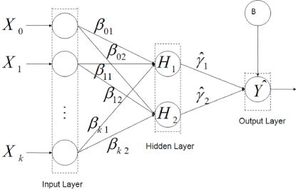
Figure 1: A FFNN with one hidden layer and one output.

A typical FFNN is depicted as follows: Algebraic form of neural network can be written

$$Y=y_{0}+\sum_{j=1}^{h}y_{j}f_{j}(X,w_{j})$$ (1)

Where $w_{j}$ is the vector of weights for $jth$ neuron , $X=(X_{1},X_{2},...,X_{k})$ is vector of explanatory variables, and $f_{j}(X,w_{j})=G(w_{0j}+X^{\prime}w_{j}),j=1,...,h$ shows output of the hidden unites. The function $G$ is any activation function such as hyperbolic tangent function $G(n)=(e^{n}-e^{-n})(e^{n}+e^{-n})^{-1}$ or logistic function $G(n)=(1+e^{-n})^{-1}$. An FFNN can compose from more than one hidden layer as well it can has multi output which is similar to system of nonlinear regression equations.

The FFNN is organized here with three layers; input, hidden, and output layers. The activation function in the first layer is log-sigmoid, and the output layer activation function is linear.Units between layers are connected by weights that are optimized for a minimum of the root mean square error(RMSE)between a known output and the predicted output. Training is the process by which the weights are adjusted according to Levenberg-Marquardt algorithm. A simplified definition of a NN is computer program that has been trained to learn the relationship between a given set of inputs and a known outputs. In general, training a NN requires an optimum network architecture and sufficient historical information about the time series. The architecture of a feed-forward network is specified by the number of neurons used in the input, hidden and output layers of the network. The input layer needs sufficient number of neurons so that the network has access to enough of the recent history of the time series. The hidden layer of the network is responsible for the nonlinear processing capability of the network and as such needs to have sufficient neurons to represent the underlying complexity of the time series. We only consider networks with one output, which is required to produce a prediction a number of years ahead of the must recent input. NNs are trained until the RMSE between the output values predicted by the network and the target output values has reached a minimum. At this point we say that the optimum result has been reached for the given situation. As applied to Sunspot Number (SSN) prediction, the RMSE was defined as

$$RMSE=\sqrt{\frac{1}{N}\sum_{i=1}^{N}(SSN_{obs}-SSN_{pred})^{2}}$$ (2)

where N is the number of training patterns, $SSN_{obs}$ and $SSN_{pred}$ are the observed and predicted (SSN) values. Generally, the time series is split into two data sets: a training set and a testing set. The training set is used to adjust the weights during training, while the testing set is used to verify the prediction performances of the network. Neural networks with large numbers of parameters are more in risk of overfitting. Overfitting is the problem of very bad predictions for the out of sample data in spite of very good results for in sample data. Here, for overcoming this problem we used early stopping method which stops training when validation set fails to reduce validation sample RMSE (Baum bau89 (1989)).

Table 1: Predicted values of sunspot number from 2008 to 2018

Year	Predicted	min	Year	Predicted	min	Year	Predicted	min
	values	RMSE		values	RMSE		values	RMSE
1986	12.68	0.060	1997	12.40	0.055	2008	14.46	0.039
1987	36.99	0.064	1998	66.74	0.053	2009	16.23	0.037
1988	86.17	0.057	1999	114.68	0.051	2010	17.91	0.049
1989	144.80	0.060	2000	132.90	0.056	2011	43.50	0.045
1990	135.97	0.055	2001	115.51	0.060	2012	57.64	0.047
1991	124.08	0.058	2002	104.19	0.055	2013	65.43	0.045
1992	92.14	0.053	2003	64.75	0.051	2014	56.74	0.042
1993	57.79	0.053	2004	42.20	0.051	2015	48.37	0.042
1994	38.55	0.051	2005	27.37	0.043	2016	18.58	0.041
1995	20.63	0.046	2006	19.94	0.039	2017	10.82	0.040
1996	11.22	0.052	2007	15.40	0.042	2018	14.17	0.041

Finally, before going on to present our results, we mention two different ways in which neural networks can be used to produce predictions. Firstly, in what we turn ”direct prediction”, the network only relies on actual known data to generate any predictions. Consequently the furthest ahead prediction obtainable is limited by the last known data point in the time series plus the predict ahead time of the individual network. Alternatively, networks can be used to predict iteratively, sometimes called multistep prediction, in which the networks’ predictions are subsequently fed back into the input layer as new data points. Potentially this allows networks to predict arbitrarily far ahead; in practice, as predicted values make up more and more of the supposedly known input data, errors can be compounded recursively until no estimate of accuracy of the results can be calculated (Conway con98 (1998)).

3 Solar indices forecasting

Here we wish to predict up to 10 years ahead, and consequently, we use yearly sunspot number since the use of monthly data would require potentially large network. Furthermore, Hoyt et al. hoy94 (1994) have shown that some of Wolf’s reconstructed values were wrong, particularly for the early cycles 1-7. Thus only the post-1850 data can be considered wholly reliable. It should be considered that cycle 23 began in 1996 May and reached its maximum in 2000 April, and now it is inferred to end in 2008 December (or probably later); therefore, its length should be 12.6 yr (or longer)(Li li09 (2009)).The sunspot number yearly mean value were obtained electronically from the website:ftp://ftp.ngdc.noaa.gov/STP/SOLAR_DATA/.

Regarding time difference between data accessing, we choose various network architecture for our time series. After a massive work of trial and error, We process sunspot number time series with a neural network of 128-42-1 structure which means we used the sunspot values for the years 1882-2009 as the training set.

For the sunspot number $R_{z}$, we obtained 2013 as the year of next maximum with a value of around 65. Regarding the accuracy of the year of maximum prediction, for the two cycles predicted with this network, in two cases the date of maximum was predicted correctly. With comparison of predicted value and observed value of Solar Cycles (SCs) 22 and 23, Uncertainty about the value of the sunspot maximum have been obtained $\pm 13$. All of the predicted values for sunspot number have been added to Table 1. Also, comparison between the 1986-2009 observed sunspot number and the predictions of neural networks are shown in figure 2 as well as the predicted shape and amplitude of SC 24 in terms of yearly sunspot number.

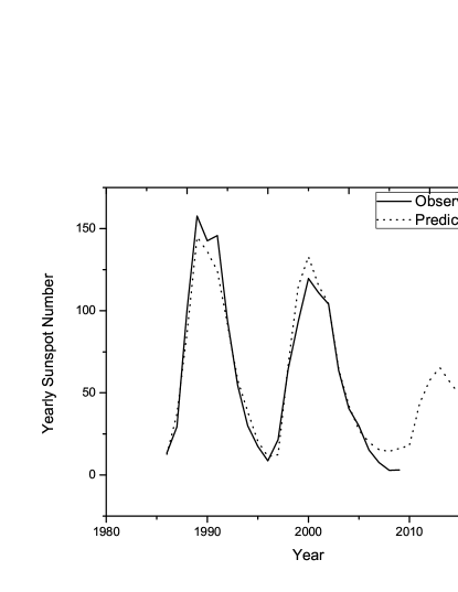
Figure 2: Observed SCs 22 and 23 (solid line) and the predicted SCs 22,23 and 24 (dashed line) in terms of yearly mean sunspot numbers.

4 Discussion and conclusions

Our neural network method is based on one hidden layer. For having reliable result, we use multi-step prediction to have only one reasonable output. In terms of processing data, by changing back-propagation algorithm to Levenberg-Marquardt algorithm our feed-forward neural network model becomes faster since LM algorithm speeds up convergence while limiting memory requirements (Battiti bat92 (1992)). We saw almost a similarity between predicted Solar cycle 24 and Solar cycle 20 . We predict a SC 24 with a maximum of $65\pm 13$ occurring in 2013. In general, our result is close to other prediction made for solar cycle 24. For example, Li et al. li05 (2005) obtained 2013 a maximum of cycle 24 with statistical method. Also a recent article by Wang et al. wang09 (2009), using similar descending phases and a cycle grouping, predicted that peak amplitude for that monthly smoothed sunspot number in the solar cycle 24 is near $100.2\pm 7.5$, occurring in 2012. Furthermore, Chumak et al. chumak10 (2010) predicted that the maximum amplitude of cycle 24 is $90\pm 20$ which is in agreement with our results. Finally, Our prediction fits well within the limits of the others as indicated in Pesnell pes08 (2008) where an average cycle was predicted using other methods such as statistical and precursor methods.

References

- (1) Battiti R., 1992, Neural Computation, 4, 141
- (2) Baum E. B., Haussler D., 1989, Neural Computation, 6, 151
- (3) Chumak O.V., and Matveychuk T.V., 2010, \chjaa, 10, 9, 935
- (4) Conway A.J., 1998, New Astronomy Reviews, 42, 343
- (5) Hagan M. T., Menhaj M., 1994, IEEE Transaction on Neural Networks, Vol.5, 6, 989
- (6) Hornik, K., Stinchcombe, M., White, H., 1989, Neural Networks, 2, 359
- (7) Hoyt, D.V., K. H. Schatten, and E.Nesmes-Ribes, 1994, Geophys. Res. Lett., 21, 2067
- (8) Koons H.C., Gorney D.J., 1990, EOS, Trans.AGU, 71, 677
- (9) Levenberg K., 1944, Quarterly of Applied Mathematics, 2(2), 164
- (10) Li K. J., 2009, \chjaa, 9, 9, 959
- (11) Li K. J., Gao P.X., and Su T.W., 2005, \chjaa, 5, 5, 539
- (12) Lundstedt H., 1992, Planet.Space.Sci., 40, 457
- (13) Marquardt D.W.,1963, SIAM Journal of Applied Mathematics, 11(2),431
- (14) Pesnell W.D., 2008, Prediction of solar cyle 24
- (15) Rumelhart D.E., Hinton G.E., Williams R.J., 1986, Nature, 323, 533
- (16) Wang J. L., Zong W.G.,Zhao H.J., Tang Y.Q., and Zhang Y., 2009, \chjaa, 9, 2, 133
- (17) Weigend A.S., Huberman B.A, Rumelhart D., 1990, Int.J.Neural Syst., 1,193