A survey of the Poincaré Center Problem in degree 3 using finite field heuristics

Abstract.

We compare a heuristic count of components of the center variety in degree $3$ with the equivalent count obtained from known families. From this comparison we conjecture that more than 100 unknown components exist.

1. Introduction

In 1885 Poincaré asked when the differential equation

$$y^{\prime}=-\frac{x+p(x,y)}{y+q(x,y)}=:-\frac{P(x,y)}{Q(x,y)}$$

with convergent power series $p(x,y)$ and $q(x,y)$ starting with quadratic terms, has stable solutions in the neighborhood of the equilibrium solution $(x,y)=(0,0)$. This means that in such a neighborhood the solutions of the equivalent plane autonomous system

$$\dot{x} =y+q(x,y)=Q(x,y)$$

$$\dot{y} =-x-p(x,y)=-P(x,y)$$

are closed curves around $(0,0)$.

Poincaré showed that one can iteratively find a formal power series $F=x^{2}+y^{2}+f_{3}(x,y)+f_{4}(x,y)+\dots$ such that

$$\det\begin{pmatrix}F_{x}&F_{y}\\ P&Q\end{pmatrix}=\sum_{j=1}^{\infty}s_{j}(x^{2j+2}+y^{2j+2})$$

with $s_{j}$ rational polynomials in the coefficients of $P$ and $Q$. If all $s_{j}$ vanish, and $F$ is convergent then $F$ is a constant of motion, i.e. its gradient field satisfies $Pdx+Qdy=0$. Since $F$ starts with $x^{2}+y^{2}$ this shows that close to the origin all integral curves are closed and the system is stable. Therefore the $s_{j}$’s are called the focal values of $Pdx+Qdy$. Often also the notation $\eta_{2j}:=s_{j}$ is used, and the $\eta_{i}$ are called Lyapunov quantities.

Poincaré also showed, that if an analytic constant of motion exists, the focal values must vanish. Later Frommer [Fro34] proved that the systems above are stable if and only if all focal values vanish even without the assumption of convergence of $F$. (Frommer’s proof contains a gap which can ben be closed [vW05])

Unfortunately it is in general impossible to check this condition for a given differential equation because there are infinitely many focal values. In the case where $P$ and $Q$ are polynomials of degree at most $d$, the $s_{j}$ are polynomials in finitely many unknowns. Hilbert’s Basis Theorem then implies that the ideal $I_{\infty}=(s_{1},s_{2},\dots)$ is finitely generated, i.e there exists an integer $m:=m(d)$ such that

$$s_{1}=s_{2}=\dots=s_{m(d)}=0\implies s_{j}=0\quad\forall j.$$

This shows that a finite criterion for stability exists, but due to the indirect proof of Hilbert’s Basis Theorem no value for $m(d)$ is obtained. In fact even today only $m(2)=3$ is known. In [vBK09] we prove $m(3)\geq 13$ for complex centers.

The proof for $m(2)=3$ is conceptually simple: Compute the first $3$ focal values as polynomials in the coefficients of $P$ and $Q$ under the assumption $\deg(P)=\deg(Q)=2$. The $3$ polynomials cut out an algebraic variety in the space of all differential equations of degree $2$. Then decompose, by hand or by computer, this variety into its irreducible components. For each component prove that all its differential equations have a constant of motion.

For $d=3$ this approach is not feasible because the polynomials $s_{j}$ are very large. They involve $14$ variables and are of weighted degree $2j$. For example the $s_{6}$ can be calculated with our script s6 available at [vBK10b] and has already $95760$ terms. The polynomials $s_{j}$, $j\geq 7$ are hard to calculate. Even if we would somehow obtain these polynomials, it is extremely difficult to decompose the resulting variety into irreducible components. Even $I_{5}=(s_{1},\dots,s_{5})$ can not be decomposed by current systems. So for $d=3$ only partial results are known, for example [CRŻ97] and [Chr05]. In [Żoł96] Żoła̧dek gives a list of $52$ families of differential forms known to have a center.

Our main tool is a statistical method of Schreyer [vBS05] to estimate the number of components of the locus $Z_{i}$ where the first $i$ focal values vanish. The basic idea is to reduce the equations $s_{k}$ modulo a prime number $p$ and count the number of $\mathbb{F}_{p}$-rational points of $Z_{i}$ with a tangent spaces of fixed codimension. By the Weil Conjectures [Wei49], which were proved by Delinge [Del74], we know that the fraction of points

$$\gamma_{p}(Z_{i}^{c}):=\frac{\#\{\text{$\mathbb{F}_{p}$ rational points on $Z_{i}$ with $\operatorname{codim}T_{Z,z}=c$}\}}{p^{14}}$$

is equal to

$$r\Bigl{(}\frac{1}{p}\Bigr{)}^{c}+\text{higher order terms}$$

for a disjoint union of $r$ smooth codimension $c$ varieties. If the components of $Z_{i}$ are not smooth and disjoint, this number is expected to be smaller. More precisely, if the set of singular points has $r_{s}$ components of codimension $c_{s}$ in the codimension $c$ components of $Z$, we expect by the same reasoning that the fraction of singular points

$$\gamma_{p}(\operatorname{sing}(Z_{i}^{c})):=\frac{\#\{\text{$\mathbb{F}_{p}$ rational singular points on $\operatorname{codim}c$ components of $Z_{i}$}\}}{p^{14}}$$

is equal to

$$r_{s}\Bigl{(}\frac{1}{p}\Bigr{)}^{c+c_{s}}+\text{higher order terms}.$$

If $r_{s}$ is small with respect to $p^{c_{s}}$ this error does not change the expected number $\gamma_{p}(Z_{i}^{c})$ significantly.

Instead of evaluating the $s_{k}$ at all possible points, we look at a large number of random points and obtain an approximate value of $\gamma_{p}(Z_{i}^{c})$ that can be used to estimate $r$ and therefore give an indication of the number of components in codimension $c$. All this is reviewed in Section 3.

In Section 4 we apply the above method using our implementation of Frommers Algorithm. The resulting estimates can be found in Figure 1.

In Section 5 we analyse Żoła̧dek’s families in detail. We choose random points on each family and apply the same statistic as above. Here we find that most families are either parametrizing non-reduced components of $Z$ or subvarieties of true components. Only 22 families seem to parametrize reduced components of $Z$. Those components can be found in Figure 6.

Comparing this to our estimate from Section 4 we find that up to codimension $7$ both counts agree. In codim $8$ we found heuristic evidence for $4$ components in Section 4 while in Żoła̧dek’s list we find $5$ such components. This apparent contradiction is resolved by showing that two of Żoła̧dek’s codimension $8$ families ($CR_{4}$ and $CR_{6}$) contain the same differential forms. For codimension $9$, $10$ and $11$ the heuristic method predicts many more reduced components than those that are contained in Żoła̧dek’s lists. We therefore conjecture that there are many more components to be discovered (see Conjecture 5.26).

The computations for this article were done at the Gauss Laboratory at the University of Göttingen. The source code for the Macaulay2 calculations of Section 5 is contained in survey2.m2 using the packages CenterFocus and Frommer. These files and the source code for our C++ Implementation of Frommers Algorithm can be found at [vBK10b]. Macaulay2 is available at [GS].

2. Preliminaries

If not stated otherwise we work over an algebraically closed field in this paper.

We write the differential equation

$$y^{\prime}=-\frac{P(x,y)}{Q(x,y)}$$

as $P(x,y)dx+Q(x,y)dy=0$.

Notation 2.1.

Furthermore we denote by

$V$	the $20$ dimensional space of degree $3$ differential forms $Pdx+Qdy$.
$W$	the $14$ dimensional subspace of Poincaré differential forms
	$(x+P_{2}(x,y)+P_{3}(x,y))dx+(y+Q_{2}(x,y)+Q_{3}(x,y))dy$

Definition 2.2.

The group

$$G:=\operatorname{Aff}_{2}:=\left\{\begin{pmatrix}M&v\\ 0&1\end{pmatrix}\,|\,\det M\not=0\right\}\subset GL(3)$$

with $M=\bigl{(}\begin{smallmatrix}m_{11}&m_{21}\\ m_{12}&m_{22}\end{smallmatrix}\bigr{)}$ and $v=\bigl{(}\begin{smallmatrix}v_{1}\\ v_{2}\end{smallmatrix}\bigr{)}$ is called the affine linear group. $G$ acts on the space of differential forms $V$ by affine linear transfomations, i.e. for $g\in G$

$$g\begin{pmatrix}x\\ y\end{pmatrix} =M\cdot\begin{pmatrix}x\\ y\end{pmatrix}+v$$

$$g\begin{pmatrix}dx\\ dy\end{pmatrix} =M\cdot\begin{pmatrix}dx\\ dy\end{pmatrix}$$

The subgroup

$$O(2):=\left\{\begin{pmatrix}M&0\\ 0&1\end{pmatrix}\,|\,MM^{T}=\begin{pmatrix}1&0\\ 0&1\end{pmatrix}\right\}\subset G;$$

is called the orthogonal group. $O(2)$ acts on $W$ since it fixes the linear part $xdx+ydy=\frac{1}{2}D(x^{2}+y^{2})$.

Definition 2.3.

A differential form $\omega=Pdx+Qdy\in V$ has a zero in $a$ if $P(a)=Q(a)=0$. We say that $Pdx+Qdy$ has a center at $a$ if in addition there exist formal power series $\mu$ and $F$ centered at $a$ such that $\mu(a)\not=0$ and $dF=\mu\omega$. In this case $\mu$ is called an integrating factor and $F$ a first integral.

Lemma 2.4.

If $\omega$ has a center at $a$ then $d\omega(a)=0$.

Proof.

If $\omega$ has a center at $a$, there exist $\mu$ and $F$ with $dF=\mu\omega$ as above. Applying $d$ to this equation we obtain

$$0=ddF=(d\mu)\omega+\mu(d\omega)$$

Evaluating at $a$ yields

$$0=(d\mu)(a)\omega(a)+\mu(a)(d\omega)(a)=\mu(a)(d\omega)(a)$$

since $\omega(a)=0$. Now $\mu(a)\not=0$ by definition, so we obtain $(d\omega)(a)=0$. ∎

Lemma 2.5.

If a differential form $\omega$ has a center at $a$ then there exists a first integral $F$ at $a$ whose Taylor expansion at $a$

$$F=F_{a,0}+F_{a,1}+F_{a,2}+\dots$$

satisfies $F_{a,0}=F_{a,1}=0$.

Proof.

$\omega$ has a first integral since it has a center at $a$. Since in the definition of first integral only $dF$ appears one can set $F_{a,0}=0$ without loss of generality. Now $F_{a,i}$ are homogeneous polynomials of degree $i$ in $(x-a_{x})$ and $(y-a_{y})$. Therefore $dF_{i}(a)=0$ for all $i\not=1$. Now $F_{1}=\alpha(x-a_{x})+\beta(y-dy)$ for certain $\alpha$ and $\beta$. We obtain

$$\alpha dx+\beta dy=dF_{1}(a)=dF(a)=(\mu\omega)(a)=0$$

and conclude $F_{1}=0$. ∎

Definition 2.6.

In the situation of Lemma 2.5, $F_{2,a}=:F_{2}(\omega,a)$ is called the quadric associatied to $\omega$ in $v$. The rank of $F_{2}(\omega,a)$ is invariant under affine coordinate tranformations.

Remark 2.7.

If $\omega$ has a center at $(0,0)$ and $\operatorname{rank}F_{2}(\omega,(0,0))=2$ we can assume that $F$ has no constant or linear terms as above. Over an algebraically closed field we can find a coordinate change such that

$$F=\frac{1}{2}(x^{2}+y^{2})+\dots$$

and $\omega=xdx+ydy+\dots$, i.e $\omega$ is a Poincare differential form.

Over an arbitrary field this is only possible if additional conditions are satisfied. For example over $\mathbb{R}$ one must assume that the quadratic form associated to $F_{2}$ is positive definite.

Definition 2.8.

Let $Pdx+Qdy$ be a Poincaré differential form of degree $3$ over a field of characteristic $0$. One can then use Frommer’s algorithm to find a formal power series $F\in K[[x,y]]$ with

$$\det\begin{pmatrix}F_{x}(x,y)&F_{y}(x,y)\\ P(x,y,1)&Q(x,y,1)\end{pmatrix}=\sum_{j=1}^{\infty}s_{j}(P,Q)(x^{2j+2}+y^{2j+2}).$$

In this situation $s_{j}(P,Q)$ is called the $j$th focal value of $Pdx+Qdy$. Frommer’s algorithm also implies that $s_{j}$ is polynomial on $W$ and has rational coefficients. We call $s_{j}\in\mathbb{Q}[p_{ij},q_{ij}]$ the $j$th focal polynomial.

Remark 2.9.

By analysing Frommer’s Algorithm [vBC07] one can show no prime factor of that the denominator of $s_{j}$ is bigger than $2j+2$. Therefore $s_{j}\mod p$ is well defined for $j\leq(p-3)/2$.

Definition 2.10.

We define the ideals

$$I_{j}=(s_{1},\dots,s_{j}),\quad I_{\infty}=(s_{1},s_{2},\dots)$$

and their vanishing sets $Z_{j}=V(I_{j})\subset W$. $Z_{\infty}$ is a variety whose points are exactly the Poincaré differential forms with a center at $(0,0)$. We therefore call it the center variety.

Remark 2.11.

In the case of degree 3 differential forms considered here, $\mathbb{Q}[p_{ij},q_{ij}]$ has 14 variables. Hilbert’s Nullstellensatz implies that $I_{\infty}$ can be generated by finitely many elements, therefore there exist a number $m:=m(3)$ such that $Z_{\infty}=Z_{m}$ and $Z_{\infty}\not=Z_{m-1}$. The precise value of $m(3)$ is unknown. In [vBK09] the inequality $m(3)\geq 13$ is proven for complex centers. Since one can not study $Z_{\infty}$ explicitly we analyze $Z_{13}$ in this paper. If $m(3)=13$ this is equivalent to analyzing $Z_{\infty}$. Otherwise we have $Z_{\infty}\subset Z_{13}$.

3. Finite Field Heuristics

In this section we explain how one can obtain heuristic information about a variety $X\subset\mathbb{A}^{n}$ by evaluating its defining equations at random points. For an extended discussion about this method see [vBS05] or [vB08]. An application of this method to the Poincaré center problems in some solved and some unsolved cases is described in [vB07].

Definition 3.1.

Let $X\subset\mathbb{A}^{n}(\mathbb{F}_{p})$ be an algebraic variety. Denote the number of $\mathbb{F}_{p}$-rational points of $X$ by $|X(\mathbb{F}_{p})|$. Then

$$\gamma_{p}(X)=\frac{|X(\mathbb{F}_{p})|}{|\mathbb{A}^{n}(\mathbb{F}_{p})|}$$

is called the fraction of $\mathbb{F}_{p}$-rational points of $X$ in $\mathbb{A}^{n}$.

Remark 3.2.

If $X$ has $r$ irreducible reduced smooth components of codimension $c$ and all other irreducible components have larger codimension then the Weil-Conjectures imply that

$$\gamma_{p}(X)=r\Bigl{(}\frac{1}{p}\Bigr{)}^{c}+\text{higher order terms in $\frac{1}{p}$}$$

We will estimate $\gamma_{p}(X)$ statistically by evaluating the equations defining $X$ in a number of randomly chosen points.

Definition 3.3.

Let $X\subset\mathbb{A}^{n}(\mathbb{F}_{p})$ be an algebraic variety. For a sequence $S=(x_{1},\dots,x_{N})$ of $\mathbb{F}_{p}$-rational points in $\mathbb{A}^{n}(\mathbb{F}_{p})$ we call

$$\tilde{\gamma}_{p}(X,S)=\frac{|\{i\,|\,x_{i}\in X\}|}{N}$$

the empirical fraction of $\mathbb{F}_{p}$-rational points.

Remark 3.4.

The distribution of $\tilde{\gamma}_{p}(X,S)$ on the set of all sequences $S$ of length $N$ is binomial with mean $\mu(\tilde{\gamma}_{p}(X,S))=\gamma_{p}(X)$ and standard deviation

$$\sigma(\tilde{\gamma}_{p}(X,S))=\sqrt{\frac{\gamma_{p}(X)(1-\gamma_{p}(X))}{N}}\approx\sqrt{\frac{\gamma_{p}(X)}{N}}$$

This allows us to obtain an estimate of $\gamma_{p}(X)$ and then of $r$ and $c$ by evaluating the equations of $X$ in many random points. More information is obtained, if we also calculate the tangent space of $X$ in these random points:

Definition 3.5.

Let $X\subset\mathbb{A}^{n}$ be an algebraic variety defined by $f_{1}=\dots=f_{r}=0$. Then the tangent space of $X$ in a point $x\in X$ is defined as

$$T_{X,x}=\ker\Bigl{(}\frac{df_{i}}{dx_{j}}(x)\Bigr{)}_{i=1\dots r,j=1\dots n}.$$

Remark 3.6.

Let $X^{\prime}\subset X\subset\mathbb{A}^{n}$ be an irreducible component, $x\in X^{\prime}$ a point and $T_{X^{\prime},x}$ the tangent space of $X^{\prime}$ in $x$. Then

$$\operatorname{codim}X^{\prime}\geq\operatorname{codim}T_{X^{\prime},x}$$

with equality for general points if $X^{\prime}$ is reduced. We therefore consider only points with $\operatorname{codim}T_{X^{\prime},x}=c$ in estimating the number of components of codimension $c$. By the inequality above we disregard all points on components of codimension greater then $c$.

These arguments lead us to

Heuristic 3.7.

Evaluate the equations of $X$ in $N$ random points $x_{i}$ over $\mathbb{F}_{p}$ and calculate the tangent spaces $T_{X,x_{i}}$ in these points. Then estimate

$$\#\{\text{reduced codim $c$ components}\}\approx\frac{\#\{i\,|\,\operatorname{codim}T_{X,x_{i}}=c\}}{N}p^{c}$$

with an estimated error

$$\Phi\frac{\sqrt{\#\{i\,|\,\operatorname{codim}T_{X,x_{i}}=c\}}}{N}p^{c}.$$

In this paper we have used $\Phi=2$ to obtain a confidence level of approximately $95\%$.

Caution 3.8.

Let $X^{c}$ be the subvariety of $X$ whose points have a tangent space of codimension $c$. Then above heuristic means that statistically the hypothesis $\gamma_{p}(X^{c})=r(1/p)^{c}$ can not be rejected with confidence of more than $4.6\%$. Algebraically this proves nothing, but gives a way to arrive at a reasonable conjecture about $X$.

Caution 3.9.

It is possible that $X$ contains a component $Y$ that is irreducible over $\mathbb{Q}$ but decomposes into several irreducible components $Y_{1},\dots,Y_{k}$ over the algebraic closure $\overline{\mathbb{Q}}$, i.e. the Galois group $\operatorname{Gal}(\overline{\mathbb{Q}}/\mathbb{Q})$ acts transitively on the $Y_{i}$. Over a finite field a $Y_{i}$ is rational if the Frobenius endomorphism fixes $Y_{i}$. The expected number of such components is $1$. Therefore our heurisic is an indication of the number of reduced irreducible components over $\mathbb{Q}$ and not over $\overline{\mathbb{Q}}$ or $\mathbb{C}$.

Remark 3.10.

If the components of $X$ are not smooth and disjoint, then

$$\frac{\#\{i\,|\,\operatorname{codim}T_{X,x_{i}}=c\}}{N}p^{c}$$

is expected to be smaller than the actual number of reduced codim $c$ component. More precisely, if the set of singular points has $r_{s}$ components of codimension $c_{s}$ in the codimension $c$ components of $X$, we expect by the same reasoning that the number of singular points on codim $c$ components to be approximately

$$\frac{r_{s}N}{p^{c+c_{s}}}.$$

If $r_{s}$ is small compared to $p^{c_{s}}$ our Heuristic 3.7 is therefore also useful in the presence of singularities. If not, the number calculated can still be used as a heuristic lower bound on the number of reduced components.

4. Experiments

Using the heuristics described in Section 3 one can estimate the number and codimension of reduced components of the center variety $Z_{\infty}$. For this we study $Z_{13}\supset Z_{\infty}$ as an approximation. This is possible because Frommer’s algorithm [Fro34], [vB07], [Mor00] provides a fast way to calculate the focal values of a given Poincaré differential form even though the explicit polynomial expressions for the focal values are not known.

Experiment 4.1.

We examined $402376372880300032\cong 4.02\times 10^{17}$ points over $\mathbb{F}_{29}$ and determined the rank of the Jacobi matrix if the first 13 focal values vanished using our implementation of Frommers algorithm [vBK10b].

This would take about 11 years of CPU time on a 2.3 GHz AMD Opteron Prozessor with 128 KB L1-Cache and 512 KB L2-Cache using our newes implementation of Frommers algorithm and a parametrization for the solution set of the first three focal values to speed up the process. We distributed the work to 56 processors.

The heuristic estimate derived from this experiment is shown in Figure 1. Interesting differential forms found in this and other computer experiments as well as statistics about theses experiments are collected in our online database [vBK10a].

Remark 4.2.

To test our implementation we have used it to recalculate the focal values of the examples in [Hö01]. Also the focal values of our example in [vBK09] were calculated independently by Colin Christopher using Reduce and agree with ours modulo $29$. Furthermore the fact that for most Żoła̧dek differential forms we indeed find points whose first 13 focal values vanish (see Section 5) can be interpreted as another test of our implementation.

To test the parametrization of the first thee focal values we compare the results obtained with and without using parametrization.

To ensure that our experiments can be repeated we use a pseudo random number generator and store the svn revision number of the program version used to do the calculation in our database.

Remark 4.3.

By applying elements of the group $O(2)$ to a given differential form $\omega$ over $\mathbb{F}_{29}$ we obtain further differential forms that have exactly the same properties as $\omega$. Now the group $O(2)$ has $2\cdot 28^{2}$ elements over $\mathbb{F}_{29}$ and therefore only approximately

$$\frac{29^{14}}{2\cdot 28^{2}}\approx 1.9\times 10^{17}$$

fundamentally different differential forms exist over $\mathbb{F}_{29}$. Since we choose our points randomly it can happen, that some forms that are equivalent with respect to $O(2)$ have been analysed several times. This makes no difference for our statistics, but prevents us from looking at all points even though we have made more than $1.9\times 10^{17}$ calculations. More precisely the propability of missing a general $O(2)$ orbit was

$$\left(1-\frac{1}{1.9\times 10^{17}}\right)^{4.0\times 10^{17}}\approx\exp\left(-\frac{4.0\times 10^{17}}{1.9\times 10^{17}}\right)\approx 12\%$$

for our experiment. Therefore one can expect that we have seen about $88\%$ of the fundamentally different differential forms.

$$\begin{array}[]{|c|c|c|c|}\hline\cr\operatorname{rank}&\text{points found}&\text{estimated number}&\text{error}\\ &&\text{of components}&\\ \hline\cr 1&208&0&<0.01\\ 2&61435&0&<0.01\\ 3&2506200&0&<0.01\\ 4&27367779&0&<0.01\\ 5&19681046795&1.00&<0.01\\ 6&1328814108&1.96&<0.01\\ 7&89629060&3.84&<0.01\\ 8&3082816&3.83&<0.01\\ 9&332067&11.97&.04\\ 10&31422&32.85&.37\\ 11&2556&77.50&3.07\\ 12&1&.88&1.76\\ \hline\cr\end{array}$$

Figure 1. Number of Poincaré differential forms whose first 13 focal values vanish over $\mathbb{F}_{29}$ found after shifting through 402376372880300032 random differential forms.

5. Żoła̧dek’s Lists

In [Żoł94] and [Żoł96] Żoła̧dek has given a list of 52 families

$$\phi\colon\mathbb{A}^{n}\to V$$

of degree 3 differential forms with a center. They are divided into 17 rational reversible systems and 35 Darboux integrable systems but this distinction is not needed for our survey. No claim on the completeness of this list is made.

Remark 5.1.

In [vB07] we proved that Żoła̧dek’s families $CR_{5}$ and $CR_{7}$ are subfamilies of $\overline{CD_{4}}$ and similarily $CR_{12}$ and $CR_{16}$ are subfamilies of $\overline{CD_{2}}$. We will therefore not consider them in this paper.

Remark 5.2.

Notice that the trivial Hamiltonian component of differential forms $\omega$ that satisfy

$$\omega=dF$$

for a polynomial $F$ of degree $4$, is not on Żoła̧dek’s list.

Remark 5.3.

In printing long lists of polynomials it is impossible not to introduce missprints. For this paper we have started from the implementation in Ulrich Rheins thesis [Rhe08] and made further corrections. Together we have made the following changes

• In $CR_{1}$ we changed the second occurrence of $q$ to a new variable, enlarging the family to all symmetric forms.

• For $CR_{3}$ we changed $(2a^{2}-b)$ to $(2a-b^{2})$ in the expression for $F$ and $5a/2$ to $3a$ in the expression for $H$. The first change is in [Rhe08] the second isn’t.

• For $CR_{5}$, $\dot{x}$ and $\dot{y}$ have to be exchanged in [Żoł96]. Also $l$ has to be changed to $ly$. This is already corrected in [Rhe08].

• In $CR_{11}$ a sign mistake was introduced in [Rhe08]

• For $CR_{17}$ the derivatives $\eta_{x}$ and $\eta_{y}$ were not calculated correctly in [Rhe08].

• For $CD_{17}$ the equation

  $$4\beta(\beta-1)a^{2}+4\beta(3-2\beta)a+(3-2\beta)(1-2\beta)=0$$

  must be satisfied. Fortunately the curve defined by this equation is rational and can be parametrized by

  $$a =\frac{-t_{0}^{4}+2t_{0}^{3}t_{1}-2t_{0}^{2}t_{1}^{2}-2t_{0}t_{1}^{3}+3t_{1}^{4}}{-2t_{0}^{3}t_{1}+8t_{0}^{2}t_{1}^{2}-14t_{0}t_{1}^{3}+12t_{1}^{4}}$$

  $$\beta =\frac{-6t_{0}t_{1}^{3}+12t_{1}^{4}}{-2t_{0}^{3}t_{1}+8t_{0}^{2}t_{1}^{2}-14t_{0}t_{1}^{3}+12t_{1}^{4}}.$$

  We substituted this parameterization into the expression for $CD_{17}$ set $t_{1}=1$ and considered only the numerator of the resulting expression. The parameterization was kindly computed for us by Janko Böhm [Böh10].

• For $CD_{24}$ we did not find any centers over $\mathbb{F}_{29}$

• In $CD_{25}$ the coefficient of $x^{3}$ was changed from $a$ to $\alpha$. This misprint was already corrected in [Rhe08]

• In $CD_{26}$ the division $/2$ must be erased. This was also found by [Rhe08].

• For $CD_{32}$ we did not find any centers over $\mathbb{F}_{29}$

• From $CD_{33}$ we obtain degree $4$ differentials for generic coefficients. Only in the case $a=1$ we were able to factor out another factor $x$. We therefore only use $CD_{33}$ with this additional restriction.

• Some families can be trivially enlarged by scaling with a nonzero scalar. We did this for all $CD$’s except $CD_{5}$ and $CD_{8}$ by multiplying the formula given by Żoła̧dek with the variable $aa_{16}$.

The families we used are contained in our Macaulay2 package CenterFocus [vBK10b], where we have renamed the variables $a,\dots,t,\alpha,\beta,\gamma$ to $aa_{1},\dots,aa_{19}$.

To estimate what part of our statistic in Figure 1 is explained by Żoła̧dek’s examples we need to take into account, that Żoła̧dek’s examples are general degree 3 differential forms in $V$ while we are interested in Poincaré differential forms in $W$. Over an algebraically closed field every degree 3 differential form $\omega$ with a non degenerate center can transformed into a Poincaré differential form by an affine transformation. It is the purpose of this section to formalize this process and keep track of the dimensions of the families involved.

Definition 5.4.

The affine linear group $G$ acts on the center variety. Therefore if

$$\phi\colon\mathbb{A}^{n}\to V$$

is a family of differential forms with a center, then

$$\psi\colon G\times\mathbb{A}^{n} \to V$$

$$(g,a) \mapsto(g(\phi(a)))$$

is a (possibly larger) family of differential forms with a center that is invariant under action of $G$. Furthermore

$$\overline{\operatorname{Im}\psi}\cap W$$

is a variety of Poincaré differential forms.

Remark 5.5.

$\overline{\operatorname{Im}\psi}\cap W$ can have several components $W_{i}$ of which at least one contains differential forms with a center at $(0,0)$. The subset of such differential forms is then dense inside this component.

Lemma 5.6.

Let $\phi\colon\mathbb{A}^{n}\to V$ be a morphism, and $D\phi$ its differential. If $a\in A$ is a integral point with $\operatorname{rank}(D\phi)(a))_{\mathbb{F}_{p}}=n$ then $\dim\phi$ = n.

Proof.

We have the following inequalities

$$n\geq\operatorname{rank}(D\phi)(a)\geq\operatorname{rank}((D\phi)(a))_{\mathbb{F}_{p}}=n.$$

Since the $D\phi$ drops rank only on Zariski closed subsets of $\mathbb{A}^{n}$ we also know that $D\phi$ has generically rank $n$. If follows that $\phi$ is generically locally injective and therefore $\dim\operatorname{Im}\phi=n$. ∎

Calculation 5.7.

We compared the number of variables $n$ involved in the definition of Żoła̧dek’s families with the rank of $D\phi$ in a random point $a$ using our script rankDifferential. For all families both numbers agreed. Figure 2 contains Żoła̧dek’s families sorted by $n=\operatorname{rank}D\phi=\dim\operatorname{Im}\phi$.

$$\begin{array}[]{|c|c|c|}\hline\cr n&CR&CD\\ \hline\cr 10&1&\\ 8&6,11&\\ 7&4&3\\ 6&2,14&1,2,4\\ 5&3,8,9,10,13,15&6,7\\ 4&&8,13,14,18,19,20,21,28,34,35\\ 3&&5,9,10,15,16,17,22,23,25,27,30,33\\ 2&17&11,12,24,26,29,31,32\\ \hline\cr\end{array}$$

Figure 2. Dimension of $\operatorname{Im}\phi$ for Żoła̧dek’s families

For the remaining calculations we need the following theorem on the dimension of fibers of a morphim:

Theorem 5.8.

Let $\phi\colon X\to Y$ be a morphism of irreducible varieties over an algebraically closed field. Then

$$\dim\phi^{-1}(y)\geq\dim X-\dim Y$$

for all $y\in Y$ and there exist a Zariski open subset $U\subset Y$ such that

$$\dim\phi^{-1}(u)=\dim X-\dim Y$$

for all $u\in U$. In this situation $\dim X-\dim Y$ is called the generic fiber dimension.

Proof.

[Mum88, 8, Theorems 2+3] ∎

Definition 5.9.

For a family $\phi$ we denote by $d_{1}=n-\dim\operatorname{Im}\phi$ the generic fiber dimension of $\phi$. For all Żoła̧dek families considered in this paper we have seen $d_{1}=0$ in Calculation 5.7.

Definition 5.10.

Let $\phi\colon\mathbb{A}^{n}\to V$ be a family of differential forms and $a\in\mathbb{A}^{n}$ a point. Then

$$G_{a}=\{g\in G|g(\phi(a))\in\overline{\operatorname{Im}\phi}\}$$

is called the set of irrelevant elements of $G$ with respect to $a$. Consider now the variety

$$X=\{(g,a)|g(\phi(a))\in\overline{\operatorname{Im}\phi}\}\subset G\times\mathbb{A}^{n}$$

and the projection

$$\pi\colon X\to\mathbb{A}^{n}$$

then $\pi^{-1}(a)=G_{a}$. From Theorem 5.8  we obtain that for almost all $a$

$$\dim G_{a}=\dim X-n=:d_{2}.$$

we call $d_{2}$ the generic dimension of $G_{a}$.

Calculation 5.11.

In Figure 3 we list subsets $H_{a}\subset G_{a}$ for almost all $a$ for all of Żoła̧dek rationally reversible families. That these are indeed subsets is checked by our script isIrrelevant.

$$\begin{array}[]{|c|c|c|c|c|c|}\hline\cr\text{Familiy}&H&\dim H&\dim G_{a}&n&\operatorname{codim}\\ &&&&&\operatorname{Im}\psi\cap W\\ &&&(\ref{cDimGa})&(\ref{cDimFiberPhi})&(\ref{calcDimWImgPsi})\\ \hline\cr CR_{1}&{\begin{pmatrix}\text{$m_{11}$}&0\\ 0&\text{$m_{22}$}\\ \end{pmatrix}}{\begin{pmatrix}0\\ \text{$v_{2}$}\\ \end{pmatrix}}&3&3&10&6\\ \hline\cr CR_{2}&{\begin{pmatrix}\text{$m_{22}$}&0\\ 0&\text{$m_{22}$}\\ \end{pmatrix}}{\begin{pmatrix}0\\ 0\\ \end{pmatrix}}&1&1&6&8\\ \hline\cr CR_{3}&{\begin{pmatrix}\text{$m_{11}$}&0\\ 0&\text{i$m_{11}$}\\ \end{pmatrix}}{\begin{pmatrix}0\\ 0\\ \end{pmatrix}}&1&1&5&9\\ \hline\cr CR_{4}&{\begin{pmatrix}\text{$m_{11}$}&\text{$v_{2}$}\text{$m_{11}$}{\text{$aa^{-1}_{3}$}}\\ 0&\text{$v_{2}$}\text{$m_{11}$}{\text{$aa^{-1}_{3}$}}+\text{$m_{11}$}\\ \end{pmatrix}}{\begin{pmatrix}0\\ \text{$v_{2}$}\\ \end{pmatrix}}&2&2&7&8\\ \hline\cr CR_{5}&\lx@intercol\hfil\text{subfamily of $CD_{4}$ \cite[cite]{[\@@bibref{}{zentrum}{}{}]}}\hfil\lx@intercol\vrule\lx@intercol\\ \hline\cr CR_{6}&{\begin{pmatrix}\text{$m_{11}$}&\text{$v_{2}$}\text{$m_{11}$}{\text{$aa^{-1}_{3}$}}\\ 0&\text{$m_{22}$}\\ \end{pmatrix}}{\begin{pmatrix}0\\ \text{$v_{2}$}\\ \end{pmatrix}}&3&3&8&8\\ \hline\cr CR_{7}&\lx@intercol\hfil\text{subfamily of $CD_{4}$ \cite[cite]{[\@@bibref{}{zentrum}{}{}]}}\hfil\lx@intercol\vrule\lx@intercol\\ \hline\cr CR_{8}&{\begin{pmatrix}\text{$m_{22}$}&0\\ 0&\text{$m_{22}$}\\ \end{pmatrix}}{\begin{pmatrix}0\\ 0\\ \end{pmatrix}}&1&1&5&9\\ \hline\cr CR_{9}&{\begin{pmatrix}\text{$m_{22}$}&0\\ 0&\text{$m_{22}$}\\ \end{pmatrix}}{\begin{pmatrix}0\\ 0\\ \end{pmatrix}}&1&1&5&9\\ \hline\cr CR_{10}&{\begin{pmatrix}\text{$m_{22}$}&0\\ 0&\text{$m_{22}$}\\ \end{pmatrix}}{\begin{pmatrix}0\\ 0\\ \end{pmatrix}}&1&1&5&9\\ \hline\cr CR_{11}&{\begin{pmatrix}\text{$m_{11}$}&\text{$v_{2}$}\text{$m_{11}$}{\text{$aa^{-1}_{3}$}}\\ 0&\text{$v_{2}$}\text{$m_{11}$}{\text{$aa^{-1}_{3}$}}+\text{$m_{11}$}\\ \end{pmatrix}}{\begin{pmatrix}0\\ \text{$v_{2}$}\\ \end{pmatrix}}&2&2&8&7\\ \hline\cr CR_{12}&\lx@intercol\hfil\text{subfamily of $CD_{2}$ \cite[cite]{[\@@bibref{}{zentrum}{}{}]}}\hfil\lx@intercol\vrule\lx@intercol\\ \hline\cr CR_{13}&{\begin{pmatrix}\text{$m_{22}$}&0\\ 0&\text{$m_{22}$}\\ \end{pmatrix}}{\begin{pmatrix}0\\ 0\\ \end{pmatrix}}&1&1&5&9\\ \hline\cr CR_{14}&{\begin{pmatrix}\text{$m_{22}$}&0\\ 0&\text{$m_{22}$}\\ \end{pmatrix}}{\begin{pmatrix}0\\ 0\\ \end{pmatrix}}&1&1&6&8\\ \hline\cr CR_{15}&{\begin{pmatrix}\text{$m_{22}$}&0\\ 0&\text{$m_{22}$}\\ \end{pmatrix}}{\begin{pmatrix}0\\ 0\\ \end{pmatrix}}&1&1&5&9\\ \hline\cr CR_{16}&\lx@intercol\hfil\text{subfamily of $CD_{2}$ \cite[cite]{[\@@bibref{}{zentrum}{}{}]}}\hfil\lx@intercol\vrule\lx@intercol\\ \hline\cr CR_{17}&{\begin{pmatrix}1&0\\ 0&1\\ \end{pmatrix}}{\begin{pmatrix}0\\ 0\\ \end{pmatrix}}&0&0&2&11\\ \hline\cr\end{array}$$

Figure 3. Calculating the codimension of $\operatorname{Im}\psi\cap W$ for Żoła̧dek’s rationally reverible systems

Calculation 5.12.

For every rational reversible Żoła̧dek family we calculate $\dim G_{a_{0}}$ for a random element $a_{0}$ using our script idealIrrelevantElementsRandom. The results can also be found in Figure 3. Since $\dim G_{a_{0}}$ is always bigger then the generic dimension of $G_{a}$ we obtain for almost all $a\in\mathbb{A}^{n}$:

$$\dim G_{a_{0}}\geq d_{2}\geq\dim H_{a}$$

From the Figure 3 we see that for every Żoła̧dek family these inequalities have to be equalities and we can calclate $d_{2}$.

Calculation 5.13.

For every Darboux integrable Żoła̧dek family we calculate $\dim G_{a_{0}}$ for a random element using our script idealIrrelevantElementsRandom. We obtain that this dimension is zero for all $CD_{i}$. Since

$$\dim G_{a_{0}}\geq d_{2}\geq 0$$

We obtain $d_{2}=0$ for these cases.

Proposition 5.14.

Consider $\psi\colon G\times\mathbb{A}^{n}\to V$ as above. Then

$$\dim\operatorname{Im}\psi=n+6-d_{1}-d_{2}.$$

Proof.

Let $\psi(g,a)=g(\phi(a))$ be a generic element of $\operatorname{Im}\psi$. Then the fibere over this element is

$$F =\psi^{-1}g(\phi(a))$$

$$=\{(h,b)|h(\phi(b))=g(\phi(a)\}$$

$$=\{(h,b)|(\phi(b)=h^{-1}g(\phi(a))\}$$

$$=\{(\tilde{h},b)|\phi(b)=\tilde{h}(\phi(a))\}\subset G_{a}\times\mathbb{A}^{n}.$$

Now consider the projection

$$\pi\colon F\to G_{a}$$

For $\tilde{h}\in G_{a}$ we obtain

$$\pi^{-1}(\tilde{h})\ =\{b|\phi(b)=\tilde{h}(\phi(a))\}$$

$$=\{b|\phi(b)=\phi(a^{\prime})\}$$

$$=\phi^{-1}(a^{\prime})$$

For generic $a$ and $\tilde{h}$ we therefore have

$$\dim F=\dim G_{a}+\dim\phi^{-1}(a)=d_{1}+d_{2}$$

by Theorem 5.8. Using Theorem 5.8  again for $\psi$ and generic $F$ we get

$$\dim\operatorname{Im}\psi=\dim(G\times\mathbb{A}^{n})-\dim F=n+6-d_{1}-d_{2}$$

∎

Proposition 5.15.

Consider the variety

$$X=\{(g,\omega)|g(\omega)\in W\}\subset G\times\operatorname{Im}\psi$$

and $X_{0}\subset X$ an irreducible component. Let

$$\pi\colon X_{0} \to G$$

$$(g,\omega) \mapsto g$$

be the natural projection. In this situation all fibers of $\pi$ are isomorphic and $\pi^{-1}(id)$ is an irreducible component of $\operatorname{Im}\psi\cap W$. Furthermore this component has the dimension $\dim X_{0}-6$.

Proof.

$G$ operates on $X$ via $h(g,\omega)=(gh,h^{-1}\omega)$. Since $G$ is irreducible it also acts on every component $X_{0}\subset X$. With this operation $\pi^{-1}(h)=h^{-1}(\pi^{-1}(\operatorname{id}))$. This proves the first claim. Now

$$\pi^{-1}(\operatorname{id})=\{\omega|\omega\in W\}\cap X_{0}.$$

This proves the second claim. The third claim follows from Theorem 5.8. ∎

Lemma 5.16.

Let $X$ be the variety considerend in Proposition 5.15 and the natural morphism

$$\eta\colon X \to\mathbb{A}^{2}\times\operatorname{Im}\psi$$

$$((\begin{smallmatrix}M&v\\ 0&1\end{smallmatrix}),\omega) \mapsto(-M^{-1}v,\omega).$$

Then

$$\operatorname{Im}\eta=\{(\tilde{v},\omega)|\omega(\tilde{v})=d\omega(\tilde{v})=0\,\text{and}\,\operatorname{rank}F_{2}(\tilde{v},\omega)=2\}.$$

Proof.

If $\omega^{\prime}:=(\begin{smallmatrix}M&v\\ 0&1\end{smallmatrix})(\omega)$ lies in $W$, it satisfies $\omega^{\prime}(0)=d\omega^{\prime}(0)=0$ and $\operatorname{rank}F_{2}(0,\omega^{\prime})=2$. But then $\omega(-M^{-1}v)=d\omega(-M^{-1}v)=0$. With $\tilde{v}:=-M^{-1}v$ this shows

$$\operatorname{Im}\eta\subset\{(\tilde{v},\omega)|\omega(\tilde{v})=d\omega(\tilde{v})=0\,\text{and}\,\operatorname{rank}F_{2}(\tilde{v},\omega)=2\}.$$

Conversely consider $(\tilde{v},\omega)$ with $\omega(\tilde{v})=d\omega(\tilde{v})=0$ and $\operatorname{rank}F_{2}(\tilde{v},\omega)=2$. Then with $g=(\begin{smallmatrix}1&-\tilde{v}\\ 0&1\end{smallmatrix})$ we have $\omega^{\prime}=g(\omega)$ satisfiying $\omega^{\prime}(0)=0$. This shows that $\omega^{\prime}$ is of the form

$$\omega^{\prime}=\omega_{1}^{\prime}+\omega_{2}^{\prime}+\dots$$

with $\omega_{1}^{\prime}=dF_{2}^{\prime}$. Since $\operatorname{rank}F_{2}=2$ there exists an element $h=(\begin{smallmatrix}M&0\\ 0&1\end{smallmatrix})$ such that $h(F_{2}^{\prime})$ is $\frac{1}{2}(x^{2}+y^{2})$. It follows that

$$\omega^{\prime\prime}:=h(\omega^{\prime})=xdx+ydy+\dots$$

and $(h\circ g,\omega)$ is an element of $X$ with image $(\tilde{v},\omega)$. ∎

$$\begin{array}[]{|c|c|c|c|c|c|c|c|c|c|c|c|c|}\hline\cr&0&1&2&3&4&5&6&7&8&9&10&11\\ \hline\cr CR_{1}&&&&&&&.87&&&&&\\ CR_{2}&&&&&&&&.01&.79&&&\\ CR_{3}&&&&&&&&&&.74&&\\ CR_{4}&&&&&&&&&.81&&&\\ CR_{6}&&&&&&&&&.88&&&\\ CR_{8}&&&&&&&&&.03&&&\\ CR_{9}&&&&&&&&&&.73&&\\ CR_{10}&&&&&&&&&&.77&&\\ CR_{11}&&&&&&&&.73&&&&\\ CR_{13}&&&&&&&&&.03&&&\\ CR_{14}&&&&&&&&&.66&.09&&\\ CR_{15}&&&&&&&&&&.76&&\\ CR_{17}&&&&&&&&&&&.03&\\ \hline\cr\end{array}$$

Figure 4. Estimated number of center variety components parametrized by Żoła̧dek’s rational reversible families

$$\begin{array}[]{|c|c|c|c|c|c|c|c|c|c|c|c|c|}\hline\cr&0&1&2&3&4&5&6&7&8&9&10&11\\ \hline\cr CD_{1}&&&&&&&.01&.87&&&&\\ CD_{2}&&&&&&&&.76&&&&\\ CD_{3}&&&&&&&.84&&&&&\\ CD_{4}&&&&&&&&.77&&&&\\ CD_{5}&&&&&&&&&&&&\\ CD_{6}&&&&&&&&.03&&&&\\ CD_{7}&&&&&&&&&.87&&&\\ CD_{8}&&&&&&&&&&.93&&\\ CD_{9}&&&&&&&&&&&&\\ CD_{10}&&&&&&&&&&&.96&\\ CD_{11}&&&&&&&&&&&&\\ CD_{12}&&&&&&&&&&&&\\ CD_{13}&&&&&&&&&&&&\\ CD_{14}&&&&&&&&&.02&&&\\ CD_{15}&&&&&&&&&&&&\\ CD_{16}&&&&&&&&&&.02&&\\ CD_{17}&&&&&&&&&&&.59&\\ CD_{18}&&&&&&&&&.02&&&\\ CD_{19}&&&&&&&&&.03&&&\\ CD_{20}&&&&&&&&&.02&&&\\ CD_{21}&&&&&&&&&&.78&&\\ CD_{22}&&&&&&&&&&&&\\ CD_{23}&&&&&&&&&&.02&&\\ CD_{25}&&&&&&&&&&&.64&\\ CD_{26}&&&&&&&&&&&&\\ CD_{27}&&&&&&&&&&&.67&\\ CD_{28}&&&&&&&&&&.12&&\\ CD_{29}&&&&&&&&&&&&\\ CD_{30}&&&&&&&&&&.03&&\\ CD_{31}&&&&&&&&&&&&.84\\ CD_{33}&&&&&&&&&&&&\\ CD_{34}&&&&&&&&&&&&\\ CD_{35}&&&&&&&&&.02&&&\\ \hline\cr\end{array}$$

Figure 5. Estimated number of center variety components parametrized by Żoła̧dek’s Darboux integrable families

Lemma 5.17.

In the situation of Lemma 5.16 the fibers of

$$\eta\colon X\to\operatorname{Im}\eta\subset\mathbb{A}^{2}\times\operatorname{Im}\psi$$

are isomorphic (as varieties) to $O(2)\subset G$. In particular the components $X_{i}$ of $X$ are in $1:1$ correspondence with the components $E_{i}$ of $\operatorname{Im}\eta$ and $\dim X_{i}=\dim E_{i}+1$.

Proof.

The group $G$ acts on $\mathbb{A}^{2}\times\operatorname{Im}\psi$ via

$$h(\tilde{v},\omega)=(h(\tilde{v}),h^{-1}(\omega))$$

where for $h=(\begin{smallmatrix}M^{\prime}&v^{\prime}\\ 0&1\end{smallmatrix})$ we set

$$h(\tilde{v}):=-(M^{\prime})^{-1}(v^{\prime}+\tilde{v}).$$

With this action the morphism $\eta$ is $G$ covariant. It follows that the fiber $\eta^{-1}(v,\omega)$ is isomorphic to a fiber $\eta^{-1}(0,\omega^{\prime})$ with $\omega^{\prime}=h^{-1}(\omega)$ for an $h$ with $h(v)=0$. We have

$$\eta^{-1}(0,\omega^{\prime}) =\{M|(\begin{smallmatrix}M&v\\ 0&1\end{smallmatrix})(\omega^{\prime})\in W\wedge-M^{-1}v=0\}$$

$$=\{M|(\begin{smallmatrix}M&0\\ 0&1\end{smallmatrix})(\omega^{\prime})\in W\}.$$

This set is non empty, since $(0,\omega^{\prime})$ is in the image of $\eta$. Therefore there exists an $h^{\prime}$ such that $h^{\prime}(0,\omega^{\prime})=(0,\omega^{\prime\prime})$ with $\omega^{\prime\prime}\in W$. Now

$$\eta^{-1}(0,\omega^{\prime\prime}) =\{M|(\begin{smallmatrix}M&0\\ 0&1\end{smallmatrix})(\omega^{\prime\prime})\in W\}$$

$$=O(2)\subset G$$

since only elements with $MM^{T}=(\begin{smallmatrix}1&0\\ 0&1\end{smallmatrix})$ fix the linear part $\omega_{1}^{\prime\prime}=xdx+ydy$. ∎

Corollary 5.18.

If $\phi$ is a family of differential forms with a center whose generic element has only finitely many zeros and a center of rank $2$, then

$$\dim W\cap\operatorname{Im}\psi=n+1-d_{1}-d_{2}.$$

Proof.

By assumption a Zariski open subset of $\operatorname{Im}\phi$ contains differential forms with a rank $2$ center. Since this fact is invariant under action of $G$ the same is true for $\operatorname{Im}\psi$. For every such element $\omega\in\operatorname{Im}\psi$ one can find an element $g\in G$ such that $g(\omega)$ is a Poincaré differential form in $W$. Therefore $\xi\circ\eta$ is dominant. If $\omega$ has only finitely many zeros then $\xi^{-1}(\omega)$ is finite, so $\xi$ is generically finite by our assumptions. We obtain

$$\dim X=\dim\operatorname{Im}\psi+1.$$

Using Proposition 5.14 and Proposition 5.15 we obtain

$$\dim\operatorname{Im}\psi\cap W=\dim X-6=\dim\operatorname{Im}\psi-5=n+1-d_{1}-d_{2}.$$

∎

Calculation 5.19.

Using Corollary 5.18 we calculate $\dim W\cap\operatorname{Im}\psi$ for Żoła̧dek’s families of rationally revesible centers. The results can also be found in Figure 3. For Żoła̧dek’s families of Darboux centers we have $d_{1}=d_{2}=0$ and therefore the dimensions are equal to $n+1$ and can be read from Figure 2.

Remark 5.20.

We collect the previous definitions, lemmata and propsitions in the following diagram:

where labels of the $\xi$- and $\eta$ arrows denote the expected fibers. Special fibers could have a different structure.

To estimate the component structure of $\pi^{-1}(\operatorname{id})=\operatorname{Im}\psi\cap W$ we use again our heuristic approach.

Calculation 5.21.

Starting from a family $\phi\colon\mathbb{A}^{n}\to V$, we find rational points on $\operatorname{Im}\psi\cap W$ as follows. First choose a rational point $a\in\mathbb{A}^{n}$ and consider the differential form $\omega=\psi(\operatorname{id},a)=(\phi(a))\in\operatorname{Im}\psi$. If $v_{1},\dots,v_{k}$ are the rational symmetric zeros of $\omega$, then the rational points in the preimage of $\xi$ are

$$\xi^{-1}(\omega)=\{(v_{i},\omega)\,|\,i=1,\dots,k\}.$$

For each pair $(v_{i},\omega)\in\mathbb{A}^{2}\times\operatorname{Im}\psi$ the preimage of $\eta$ is

$$\eta^{-1}(v_{i},\omega)=\{(M,-Mv_{i},\omega_{g}\,|\,(M,-M^{-1}v_{i})(\omega)\in W\}$$

Now

$$(\begin{smallmatrix}M&-Mv_{i}\\ 0&1\end{smallmatrix})=(\begin{smallmatrix}M&0\\ 0&1\end{smallmatrix})(\begin{smallmatrix}1&-v_{i}\\ 0&1\end{smallmatrix})$$

and $\omega_{i}:=(\begin{smallmatrix}1&-v_{i}\\ 0&1\end{smallmatrix})(\omega)$ has zeros at $(v_{j}-v_{i})$ in particular one at zero. Therefore $\omega_{i}$ is of the form

$$\omega_{i}=l_{11}xdx+l_{12}(xdy+ydx)+l_{22}ydy+\text{higher order terms}$$

We have $(\begin{smallmatrix}M&0\\ 0&1\end{smallmatrix})(\omega_{i})\in W$ if and only if

$$M^{t}L_{i}M=(\begin{smallmatrix}1&0\\ 0&1\end{smallmatrix})$$

with

$$L_{i}=(\begin{smallmatrix}l_{11}&l_{12}\\ l_{21}&l_{22}\end{smallmatrix}).$$

Since by Lemma 5.17 the solution is a one dimensional space, we can fix one entry of $M$ and and generically obtain finitely many rational solutions $M_{i1},\dots,M_{il}$. In this manner we have found finitely many rational points

$$(g,\omega)\in(\eta\circ\xi)^{-1}(\omega)\subset X\subset G\times\operatorname{Im}\phi$$

with

$$g\in\{(M_{ij},-M_{ij}v_{i})\}.$$

To obtain points in $W\cap\operatorname{Im}\psi=\pi^{-1}(\operatorname{id})$ we operate with $g^{-1}$ on the whole situation, and obtain points

$$(\operatorname{id},g(\omega))\in X\subset G\times\operatorname{Im}\psi$$

The points $g(\omega)$ can then be analysed with our implementation of Frommer’s algorithm. If the first $13$ focal values of $g(\omega)$ vanish we calculate the codimension of the tangent space to $Z_{13}\supset Z_{\infty}$ in these points. The results of doing this for $2000$ random choices of $a$ in each of Żoła̧dek’s   families are available as hash tables experimentsCR and experimentsCD in survey2.m2. For the families $CD_{24}$ and $CD_{32}$ we did not find any differential forms this way.

We now want to identify those Żoła̧dek -families that define reduced components of the center variety $Z_{13}\supset Z_{\infty}$. For this we use again our finite field heuristic.

Calculation 5.22.

Consider a family $\phi\colon\mathbb{A}^{n}\to V$ and set $d=W\cap\operatorname{Im}\psi$. $W$ might have several components $W_{i}$ of which at least one has dimension $d$. By the procedure above we expect to find approxemately $2000/p^{d-\dim W_{i}}$ points on a component $W_{i}$ of $W\cap\operatorname{Im}\psi$. The generic codimension of a tangent space to the center variety in points of $W_{i}$ is $14-\dim W_{i}$ if and only if $W_{i}$ is also a reduced component of the center variety. We can therefore heuristically identify reduced components of the center variety $Z_{13}$ by scaling our point counts by $p^{d-14+c}/2000$ where $c$ is the codimension of the tangent space a each point. The result is contained in Figures 4 and 5.

$$\begin{array}[]{|c|c|c|}\hline\cr\text{codim}&CR&CD\\ \hline\cr 6&1&3\\ 7&11&1,2,4\\ 8&2,4,6,14&7\\ 9&3,9,10,15&8,21\\ 10&&10,17,25,27\\ 11&&31\\ \hline\cr\end{array}$$

Figure 6. Żoła̧dek families that heuristically parametrize reduced components of the center variety

Remark 5.23.

A family $\phi$ will have all numbers calculated above close to zero if one of the following holds

1. $\phi$ defines only a subfamily of a true component of the center variety and the codimension of the family inside the component is at least one.

2. $\phi$ defines a non reduced component of the center variety

3. The generic point of $\phi$ does not have a symmetric center.

We suspect that all three possibilities actually occur. The third case can be easily detected by analysing a generic point. This shows that families $CD_{33}$ and $CD_{34}$ are of this kind. Probably this is either due to misprints introduced by us or by misprints in [Żoł94] or [Żoł96] that we were not able to find and correct.

To distinguish between the cases (1) and (2) is much more difficult.

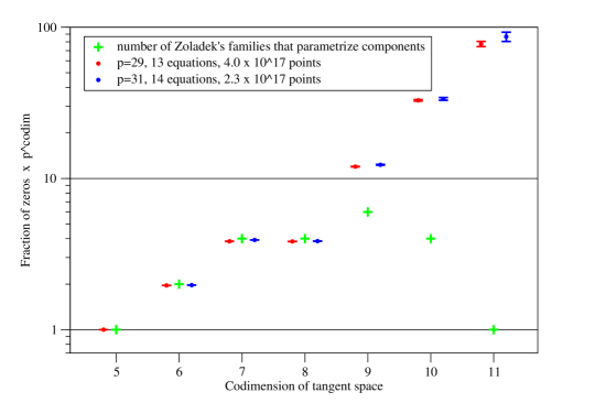
Figure 7. Our heuristic predicts that up to codimension 8 all reduced components of the center variety are known. For higher codimension many components are waiting to be discovered.

Remark 5.24.

Notice that only smooth points on each components have the correct tangent dimenesion. Therefore we expect the results of the above scaling to be less than $1$ for each component of the center variety. We have collected those families that do parametrize a reduced component of the center variety by this heuristic in Figure 6.

Comparing the number of components contained in Figure 6 with those of Figure 1 we find that up to codim 7 both counts agree in codim 8 there are 5 components given by Żoła̧dek , while we see only 4 in our heuristic. Fortunately Ulrich Rhein has found numerical evidence for $CR_{4}\subset CR_{6}$ in his Diploma Thesis [Rhe08]. It is not difficult to prove that this is indeed the case:

Proposition 5.25.

All differentials parametrized by Żoła̧dek’s family $CR_{4}$ are also contained in Żoła̧dek’s family $CR_{6}$.

Proof.

One can obtain $CR_{4}$ from $CR_{6}$ by setting $k=0$ and renaming the variables as follows $r\to q\to p\to n\to l\to k$ in Żoła̧dek’s notation. ∎

With this correction we have compared our heuristic component count with the components detected among Żoła̧dek’s list in Figure 7. We observe, that up to codimension $8$ both counts agree. Starting from codimension $9$ there seem to exist many more reduced components than previously known. We therefore

Conjecture 5.26.

The number of reduced components of the center variety in degree $3$ is

• 1 in codimension 5

• 2 in codimension 6

• 4 in codimension 7

• 4 in codimension 8

• at least 12 in codimension 9

• at least 33 in codimension 10

• at least 74 in codimension 11

• possibly further components in codimension 12

Remark 5.27.

The Macaulay2 calculations made in this section are contained in the file survey2.m2 using the packages CenterFocus and Frommer. All three are available at [vBK10b]. Macaulay2 is available at [GS].

References

- [Böh10] Janko Böhm. Parametrization, a macaulay2 package for computing rational parametrizations of rational curves. Available at http://www.math.uni-sb.de/ag/schreyer/jb/Macaulay2/Parametrization/html/, 2010.
- [Chr05] Colin J. Christopher. Centre conditions for a class of polynomial differential systems. preprint, 2005.
- [CRŻ97] L. A. Cherkas, V. G. Romanovskii, and H. Żoła̧dek. The centre conditions for a certain cubic system. Differential Equations Dynam. Systems, 5(3-4):299–302, 1997. Planar nonlinear dynamical systems (Delft, 1995).
- [Del74] P. Deligne. La conjecture de Weil, I. Publ. Math. IHES, 43:273–307, 1974.
- [Fro34] M. Frommer. Über das Auftreten von Wirbeln und Strudeln (geschlossener und spiraliger Integralkurven) in der Umgebung rationaler Unbestimmtheitsstellen. Math. Ann., 109:395–424, 1934.
- [GS] Daniel R. Grayson and Michael E. Stillman. Macaulay2, a software system for research in algebraic geometry. Available at http://www.math.uiuc.edu/Macaulay2.
- [Hö01] André Höhn. Algebraische Berechnung von Strudelgrößen und graphisches Auffinden von Grenzzykeln um eine Stelle der Unbestimmtheit. Diploma thesis, Universität Bayreuth, Germany, 2001. available online at http://www.uni-bayreuth.de/departments/math/org/mathe6/publ/da/hoehn/diplom.htm.
- [Mor00] Kay Moritzen. Ein rekursives Verfahren zur Berechnung von Strudeln für Differentialgleichungen um eine Unbestimmtheitsstelle. Diploma thesis, Universität Bayreuth, Germany, 2000. available online at http://www.uni-bayreuth.de/departments/math/org/mathe6/publ/da/moritzen/diplom.html.
- [Mum88] David Mumford. The red book of varieties and schemes, volume 1358 of Lecture Notes in Mathematics. Springer-Verlag, Berlin, 1988.
- [Rhe08] Ulrich Rhein. Das Poincarésche Zentrumsproblem: Komponenten der Zentrumsvarietät. Diploma thesis, Leibniz Universität Hannover, Germany, 2008. available online at http://www.crcg.de/wiki/Hans-Christian_Graf_v._Bothmer:_Betreute_Abschlussarbeiten#2008.
- [vB07] Hans-Christian Graf v. Bothmer. Experimental results for the Poincaré center problem. NoDEA Nonlinear Differential Equations Appl., 14(5-6):671–698, 2007.
- [vB08] Hans-Christian Graf v. Bothmer. Finite field experiments. In Higher-dimensional geometry over finite fields, volume 16 of NATO Sci. Peace Secur. Ser. D Inf. Commun. Secur., pages 1–62. IOS, Amsterdam, 2008.
- [vBC07] H.-Chr. Graf v. Bothmer and Martin Cremer. Frommers algorithm. NoDEA, 14(5-6):694–698, 2007.
- [vBK09] Hans-Christian Graf v. Bothmer and Jakob Kröker. Focal values of plane cubic centers, 2009.
- [vBK10a] H.-Chr. Graf v. Bothmer and Jakob Kröker. A database of differential forms in characteristic . Available at http://centerfocus.de/, 2010.
- [vBK10b] H.-Chr. Graf v. Bothmer and Jakob Kröker. Source files for the centerfocus project. Available at http://sourceforge.net/projects/centerfocus, 2010.
- [vBS05] H.-C. Graf v. Bothmer and F.-O. Schreyer. A quick and dirty irreducibility test for multivariate polynomials over . Experiment. Math., 14(4):415–422, 2005.
- [vW05] Wolf v. Wahl. personal communication, 2005.
- [Wei49] A. Weil. Number of solutions of equations over finite fields. Bull. Amer. Math. Soc., 55:497–508, 1949.
- [Żoł94] Henryk Żoła̧dek. The classification of reversible cubic systems with center. Topol. Methods Nonlinear Anal., 4(1):79–136, 1994.
- [Żoł96] Henryk Żoła̧dek. Remarks on: “The classification of reversible cubic systems with center” [Topol. Methods Nonlinear Anal. 4 (1994), no. 1, 79–136; MR1321810 (96m:34057)]. Topol. Methods Nonlinear Anal., 8(2):335–342 (1997), 1996.