Optical Polarization Mapping toward the interface between the Local Cavity and Loop I

Abstract

The Sun is located inside an extremely low density and quite irregular volume of the interstellar medium, known as the Local Cavity (LC). It has been widely believed that some kind of interaction could be occurring between the LC and Loop I, a nearby superbubble seen in the direction of the Galactic Center. As a result of such interaction, a wall of neutral and dense material, surrounded by a ring shaped feature, would be formed at the interaction zone. Evidence of this structure was previously observed by analyzing the soft X-ray emission in the direction of Loop I. Our goal is to investigate the distance of the proposed annular region and map the geometry of the Galactic magnetic field in these directions. On that account, we have conducted an optical polarization survey to $878$ stars from the Hipparcos catalogue. Our results suggest that the structure is highly twisted and fragmented, showing very discrepant distances along the annular region: $\approx 100$ pc to the left side and $250$ pc to the right side, independently confirming the indication from a previous photometric analysis. In addition, the polarization vectors’ orientation pattern along the ring also shows a widely different behavior toward both sides of the studied feature, running parallel to the ring contour in the left side and showing no relation to its direction in the right side. Altogether, these evidence suggest a highly irregular nature, casting some doubt on the existence of a unique large-scale ring-like structure.

1 Introduction

The Sun is located roughly at the center of a large interstellar feature in the Local spiral arm (the Orion Spur). This conspicuous structure, known as Local Cavity (LC) or Local Bubble, consists of a very irregular, low density volume ($n_{HI}<0.005$ cm^-3) of the interstellar medium (ISM), whose borders extend from $\approx 65$ to $250$pc, depending on the direction to which we observe it (Cox & Reynolds, 1987; Welsh et al., 1994; Lallement et al., 2003; Vergely et al., 2010). This cavity is surrounded by several other interstellar bubbles that are sometimes associated to strong star-forming activity, and are frequently believed to have been generated by supernovae (SN) explosions and very intense stellar winds from massive OB stars (Quigley & Haslam, 1965; Berkhuijsen et al., 1971; Weaver, 1979).

Several efforts have been made to build a tridimensional view of the LC, mainly by using Na I observations in the direction of nearby stars, which is a suitable tracer of the neutral gas (Welsh et al., 1994; Sfeir et al., 1999; Lallement et al., 2003; Vergely et al., 2010). Information on the shape and size of this structure can also be inferred from ultraviolet interstellar absorption lines (Frisch, 1981; Frisch & York, 1983; Paresce, 1984; Centurion & Vladilo, 1991; Welsh et al., 1994; Redfield & Linsky, 2000; Sallmen et al., 2008; Welsh & Lallement, 2005), interstellar reddening (Franco, 1990; Corradi et al., 1997; Corradi et al., 2004; Frisch, 2007; Reis & Corradi, 2008; Vergely et al., 2010, Reis et al. 2010, in preparation) and interstellar polarization (Tinbergen, 1982; Reiz & Franco, 1998; Heiles, 1998, 2000; Leroy, 1999). The overall shape of the LC suggests that it is being compressed due to the expansion of the neighboring bubbles, with a narrower dimension along the Galactic Plane (GP), and probably opened in the direction of the Galactic halo. Furthermore, this “chimney” structure is slightly tilted relative to the GP ($\approx 20^{\circ}$), and perpendicular to the Gould’s Belt, a large complex of young massive OB stars surrounding the Local ISM (Welsh et al., 1994; Sfeir et al., 1999; Lallement et al., 2003; Vergely et al., 2010).

In the direction of the Galactic Center, we find a particularly interesting structure known as the Loop I superbubble, which is centered at the Scorpio-Centaurus OB association (Sco-Cen, $l\approx 329^{\circ},b\approx+17.5^{\circ}$), and probably created due to its intense stellar activity (Blaauw, 1964; de Geus, 1992; Sartori et al., 2003; Preibisch & Mamajek, 2008). This neighboring interstellar bubble, located at $d\approx 130$pc and defined by a large sky-projected diameter ($\sim 115^{\circ}$), has been better revealed by radio continuum observations, which show several arc-shaped shells of interstellar material (Berkhuijsen et al., 1971; Iwan, 1980; Haslam et al., 1982; Heiles, 1998).

The proximity between the Local and Loop I bubbles led some authors to believe that some kind of interaction could be taking place between them (Cox & Reynolds, 1987; Centurion & Vladilo, 1991). In fact, by analyzing shadowing effects at the wide-angle soft X-ray survey from ROSAT ($0.25$keV), Egger & Aschenbach (1995) proposed that the collision between both bubbles led to the formation of a wall of neutral gas surrounded by a dense interstellar ring feature at the interaction zone. This conclusion was inspired by collisional models of spherical shock fronts, which revealed that a dense interacting wall would arise, encompassed by an even denser annular feature, if at least one of the interacting shells have reached the radiative stage before the collision occurred (Yoshioka & Ikeuchi, 1990). This idea was supported by an anticorrelation between the shadows from the soft X-ray maps and the neutral hydrogen (HI) emission from the local ISM (Egger & Aschenbach, 1995; Breitschwerdt et al., 2000).

Up to date, several attempts have been made to determine the distance to the supposed interacting region, leading to widely different results. Centurion & Vladilo (1991) suggested a distance of $40\pm 25$ pc, from the analysis of ultraviolet spectra to eight stars at the region defined by $315^{\circ}<l<330^{\circ}$ and $15^{\circ}<b<25^{\circ}$. Egger & Aschenbach (1995) used HI column densities data from Fruscione et al. (1994) to determine a distance of $70$ pc, defined by a jump in $N_{H}$ from $\leq 10^{20}$ cm^-2 to $\geq 7\times 10^{20}$ cm^-2 at this distance.

Using $E(b-y)$ color excess data and high resolution spectroscopy in the direction of the Southern Coalsack, Chamaeleon, and Musca dark clouds Corradi et al. (1997); Corradi et al. (2004) suggested that the interaction zone is twisted and folded, located at $120-150$ pc along this line-of-sight. As previously pointed out by Dame et al. (2001), several dark clouds ($\rho$ Oph, Lupus, R CrA, G317-4, Southern Coalsack, Chamaeleon, and Musca) are located at the same mean distance of $150$ pc, in the direction of Loop I. However, Welsh & Lallement (2005) identified the presence of an interstellar cloud in the direction of $(l,b)\approx(330^{\circ},+18^{\circ})$, at approximately $90$ pc from the Sun, suggesting that this could be part of the interface between the Local and Loop I bubbles.

Recently, Reis & Corradi (2008) used a larger sample of $E(b-y)$ color excess data distributed along the entire interface region to map the interstellar dust distribution. The analysis led to the conclusion that the expected transition from nearly $E(b-y)=0\fm 015$ to $E(b-y)\approx 0\fm 070-0\fm 100$ (which corresponds to the ring’s density, as proposed by Egger & Aschenbach, 1995), occurs at the western (left) side at $110\pm 20$pc while the eastern (right side) transition cannot be clearly defined before $280\pm 50$ pc.

Moreover, the structure of the interstellar magnetic field along the borders of the LC have been previously studied by several polarimetric surveys (Mathewson & Ford, 1970; Tinbergen, 1982; Reiz & Franco, 1998; Leroy, 1999; Heiles, 2000). It is known that the local ISM is filled by an irregular, large-scale magnetic flux of average intensity $\langle B\rangle\approx 2.2\mu$G (Heiles, 1998; Beck, 2001; Heiles & Crutcher, 2005). Although no final conclusion has been reached in relation to the dominant physical mechanism responsible for the alignment of the interstellar dust particles, it is generally accepted that in the majority of cases, grain alignment occurs with the grain’s major axis perpendicular to the magnetic field direction (Hall, 1949; Hiltner, 1949; Davis & Greenstein, 1951; Jones & Spitzer, 1967; Codina-Landaberry & Magalhaes, 1976; Purcell, 1979; Lazarian, 1995a, b; Draine & Weingartner, 1996, 1997; Fosalba et al., 2002; Lazarian, 2007). This configuration of dust grains gives rise to an anisotropic extinction which results in a partially polarized transmitted light beam from a distant star, with position angle in the same direction as the field $\mathbf{\bf{B}}$. Therefore, there is a strong correlation between the direction of the plane-of-sky projected component of $\mathbf{\bf{B}}$ and the polarization vectors, which can be used as a powerful tool to map the Galactic magnetic field, as well as to probe the nature of the interstellar dust particles.

All-sky polarization surveys exhibit a large-scale vectors distribution pattern which is generally correlated to the direction of the local interstellar structures. Specifically, it is frequently found that polarization vectors may be aligned roughly perpendicular or parallel to the interstellar filaments, depending on several physical and geometrical factors, including projection effects (Heiles, 1998; Fosalba et al., 2002; Whittet, 2003; Heiles & Crutcher, 2005). Particularly along the Galactic plane it is noted an overall distribution of polarization angles which is mainly horizontal (i.e., parallel to the plane). Such trend reflects the morphology of the local magnetic field, directed mainly along the local spiral arm. In fact, this predominant orientation along the Galactic plane vanishes when the local magnetic field is viewed face-on along its “poles” at $l\approx(80^{\circ},260^{\circ})$, which is roughly coincident with the direction of the local spiral arm.

Large-scale mappings of the magnetic field structure in other spiral galaxies show that the orientation parallel to the galactic plane is a general trend which may be attributed to differential rotation of the galactic disk and magnetic flux freezing with the interstellar matter (Zweibel & Heiles, 1997; Beck, 2002).

In this work, we present an optical polarimetric survey in the direction of the interface between the LC and Loop I. Section 2 provides a description of the observational data, as well as the reduction process. The results and analysis of the correlation between polarimetric and color excess data, as well as of the spatial distribution of the polarimetric vectors and polarization degree as a function of distance are shown on sections 3, 4 and 5. Discussion of the results is carried out on section 6 and the conclusions are shown on section 7.

2 Observational Data

The polarimetric data used in this work were collected at OPD (Observatório Pico dos Dias, LNA/MCT, Brazil) during $63$ nights distributed between 2007 August and 2009 February. We have used both the $60$cm and $1.6$m telescopes, equipped with an imaging polarimeter attached to a specially adapted CCD camera.

The polarimeter consists of a rotating half-wave retarder, a fixed analyzer, and a filter wheel. The half-wave retarder is allowed to rotate in discrete steps of $22.5^{\circ}$, so that 16 steps corresponds to a complete rotation ($360^{\circ}$). Its effect on the incident stellar light is to cause a rotation of the polarization plane of the linearly polarized component. For instance, if the stellar initial polarization angle (relative to the North Celestial Pole - NCP) is $\theta$, and $\psi$ is the angle between the retarder’s optical axis and the NCP, the outcome is a light beam with polarization angle of $2\psi-\theta$ (Serkowski, 1974).

The analyzer was a Savart plate, i.e., a birefringent double calcite prism which subdivides the incoming light beam into two orthogonally plane-polarized beams. Thereafter, both beams pass through a filter, and are simultaneously detected by the CCD, which registers the individual beams’ intensities at each position of the half-wave retarder (for a complete description of this instrument, see Magalhães et al., 1996).

Thus, the Q and U Stokes parameters are obtained by fitting a 4-cosine modulation amplitude curve (Magalhães et al., 1984; Santos, 2009), so that the polarization degree ($P$) and the polarization angle ($\theta$) may be calculated, respectively, by

$P=\frac{\sqrt{Q^{2}+U^{2}}}{I}\ \ \ \ \ \ \ \mathrm{and}\ \ \ \ \ \ \ \theta=\frac{1}{2}\arctan{U/Q}$

($I$ represents the intensity of the incident light beam). The simultaneous observation of both light beams allows a differential calculation of the polarization parameters, i.e., independent of the atmospheric variations.

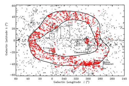
Figure 1: Polarimetric data distribution along the interface between the LC and Loop I: crosses ($\times$, colored in red at the electronic version) represent objects observed at OPD/LNA and open circles ($\circ$) represent the data acquired from Heiles (2000) catalogue. The thick contour indicates the position of the annular feature proposed by Egger & Aschenbach (1995), and the boxes roughly delimit the position of the indicated dark clouds. The data collected at OPD are mainly concentrated along the interaction ring.

Table 1: Polarimetric data obtained at OPD.

HIP	$l(^{\circ})$	$b(^{\circ})$	d(pc)	$P_{V}(\%)$	$\theta_{gal}(^{\circ})$
88294	$355.277$	$-6.689$	$222$	$0.772\pm 0.043$	$30.4\pm 1.9$
90969	$355.998$	$-13.331$	$151$	$0.293\pm 0.023$	$6.4\pm 2.5$
94157	$355.552$	$-20.975$	$256$	$0.317\pm 0.026$	$80.8\pm 2.5$
105062	$353.880$	$-44.005$	$42$	$0.050\pm 0.024$	$28.7\pm 13.8$
105133	$350.192$	$-43.855$	$133$	$0.035\pm 0.010$	$18.6\pm 8.3$
105180	$354.923$	$-44.319$	$344$	$0.172\pm 0.028$	$67.2\pm 4.8$
105391	$354.142$	$-44.695$	$53$	$0.027\pm 0.053$	$24.5\pm 56.2$
105425	$348.398$	$-44.217$	$112$	$0.104\pm 0.029$	$139.8\pm 8.1$
105685	$352.919$	$-45.208$	$97$	$0.015\pm 0.029$	$91.0\pm 55.4$
12654	$297.063$	$-36.043$	$59$	$0.023\pm 0.013$	$168.8\pm 16.2$

Standard stars were obtained from various catalogues (Serkowski et al., 1975; Bailey & Hough, 1982; Hsu & Breger, 1982; Bastien et al., 1988; Tapia, 1988; Turnshek et al., 1990; Schmidt et al., 1992; Gil-Hutton & Benavidez, 2003) and were observed at least twice every night (two polarized and two unpolarized standard stars), in order to determine the zero-point of the polarization degree and angle. Moreover, observations of standard stars were performed by using 16 positions of the half-wave plate, to minimize the uncertainties of the computed polarimetric parameters. Program stars were observed with the usually adopted 8 positions of the half-wave plate. Instrumental polarization was mainly negligible when compared to the typical polarization errors provided by this scheme ($<0.1\%$).

The reduction of the CCD images was performed using the IRAF standard routines from the CCDRED package. The polarimetric parameters were calculated for each star, using PCCDPACK, a collection of IRAF routines specifically developed to this purpose (Pereyra, 2000). This observational scheme provided mean polarization errors of approximately $0.05$%, so that typical interstellar polarization degree values ($0.1-2$%) could be easily obtained.

The observed stars were selected from the HIPPARCOS catalogue (ESA, 1997), and are distributed toward the interface region, mainly concentrated along the proposed ring structure (Figure 1, crosses). Our goal was to obtain a stellar distribution within this feature with a maximum possible spatial uniformity. However, some observational limits were imposed, e.g., notice a lack of observed data around $(l,b)\approx(300^{\circ},-30^{\circ})$, which is very close to the south celestial pole’s line-of-sight, and therefore could not be reached by the telescope. Moreover, in order to observe the entire structure of the proposed ring, our observational nights were roughly uniformly distributed along the year, allowing each part of the feature to be observed during specific months. However, some regions coincided with bad weather seasons at OPD, providing less observing time along these regions. Besides observing along the ring, we have also chosen specific lines-of-sight in the direction of the R CrA and Southern Coalsack clouds, which are located inside the contour of the ring. A small fraction of the collected data are spread throughout these areas (see Figure 1).

To guarantee an appropriate distance precision up to $\sim 200$ pc, only stars with trigonometric parallax relative error $\Delta\pi/\pi<30$% were used. Additionally to our sample, we have also used the available polarimetric data from Heiles (2000) catalogue, restricted to objects containing distance data from the HIPPARCOS catalogue with $\Delta\pi/\pi<30$%. Their distribution is also displayed in Figure 1. The whole sample, distributed along the region delimited by the Galactic coordinates $240^{\circ}<l<60^{\circ}$, $-60^{\circ}<b<60^{\circ}$, adds up to $2271$ stars, among which $1393$ are from Heiles (2000) catalogue and $878$ objects were observed at OPD (using the Johnson’s V filter). The polarimetric data set is shown in Table 1.

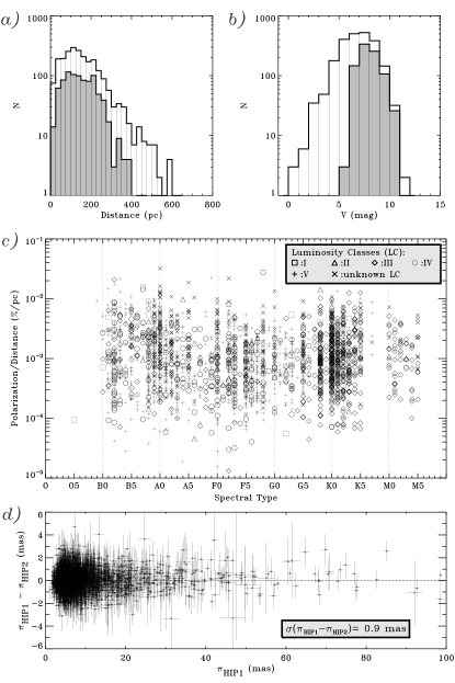
Figure 2: Histograms (a) and (b) respectively show the distributions of distance and Johnson’s V magnitude, where filled columns represent only data collected at OPD and white columns consider the entire sample (including data from Heiles (2000)). Part (c) shows a diagram of $\mathrm{P(\%)/d(pc)}\times\mathrm{Spectral\ Type}$ for the entire sample, using logarithmic scale to improve visualization and distinguishing the luminosity classes through different symbols, as shown at the gray box. Most of the stars are distributed between B and K types, and no $P/d$ trend can be seen related to giants or late-type stars, which could be associated to intrinsic polarization. The diagram from part (d) represents a measure of trigonometric paralaxes differences $(\pi_{\mathrm{HIP1}}-\pi_{\mathrm{HIP2}})$ between the Hipparcos original release (HIP1, ESA, 1997) and the new reduction provided by van Leeuwen (2007) (HIP2), using all stars from our sample. This comparison shows a small and symmetric dispersion around the equality line (the dotted line), with a standard deviation of $0.9$ milli-arcsecond (mas).

With respect to the distance distribution we have chosen stars that are mainly located between $25$ and $250$ pc, as may be seen from the histogram shown in part (a) of Figure 2. The filled portion of the histogram corresponds to the data collected at OPD, while the white columns represent the entire sample (which includes the data from Heiles (2000)). Based on the previous knowledge that the dense interstellar structures from the interface would be located between $\sim 80$ and $180$ pc, this represents a suitable distribution allowing the detection of many of these clouds. Beyond $250$ pc there is a steep decrease in the number of observed stars.

We have also plotted a histogram of the Johnson’s V magnitude (Figure 2b) for the entire sample (white portion) and more specifically to the objects observed at OPD (filled parts). Notice that most of the stars observed at OPD have $V>6$, which is related to the saturation limit of the CCD used. Our sample is limited to a maximum V magnitude of $\sim 11-12$ mag, i.e., most of the objects are bright stars.

Figure 2c shows a diagram of $\mathrm{P(\%)/d(pc)}\times\mathrm{Spectral\ Type}$, where we have used a logarithmic scale in order to obtain a better visualization, and luminosity classes are indicated by different symbols. Spectral types are mainly distributed between B and K types, reflecting the general trend for objects of the Galactic disk. No trend for specific $P/d$ values is noted toward giants or late type stars, which could indicate the presence of intrinsic polarization. Concerning such topic, it is possible that some of the objects of our sample present this property. However, we do not believe that this would alter the general picture provided by our study. Specifically, as will be shown in sections 4 and 5, it is improbable that intrinsic polarization could explain the large-scale correlation of polarization angles, and also the correlated distances where a rise in polarization degree and color excess is seen in the direction of several regions. Using the SIMBAD object classification tool for the entire sample, only six stars are designated pre-main sequence stars, namely: HIP 80337, HIP 80462, HIP 6494, HIP 93368, HIP 64408 and HIP 110778. Among these, HIP 6494 and HIP 93368 were observed at OPD, while the others were obtained from Heiles (2000).

Figure 3: Comparison between polarimetric data from Heiles (2000) catalogue and those obtained at OPD for some objects of the sample. The dashed lines were inserted for clarity, and for the $\theta$ (equatorial) comparison, only objects with $\Delta P/P<20$% were included in order to exclude the unpolarized stars.

We have used the original data from Hipparcos (HIP1, ESA (1997)), instead of the new reduction data provided by van Leeuwen (2007) (HIP2). Since a comparison of trigonometric parallaxes between both catalogs reveal a small and symmetric dispersion around the equality line for the stars of our sample (see Figure 2d), the analysis is not affected by the new reduction scheme, i.e., if small shifts would increase and decrease the distances of individual stars, this would not change the general picture provided by our results.

As a means of verifying the consistency of the collected data, some of the observed stars were chosen to match objects available from Heiles (2000) catalogue. Figure 3 shows a comparison of the polarization degree and angle for both samples. The mean percentage difference between the compared values is only $\sim 13$% for $P_{V}$ and $\sim 16$% for $\theta$.

3 Correlation between $P(\%)$ and $E(b-y)$

Whenever polarization degree is plotted against interstellar reddening, it is observed to exist a maximum value of $P$, empirically corresponding to the inequality $P_{V}/E(B-V)<9.0\%\mathrm{mag}^{-1}$ (Serkowski et al., 1975). This comes from the fact that (after the passage through a successive number of interstellar clouds) reddening of stellar light is an additive effect, whereas polarization exhibits a more complex behavior, heavily dependent on the alignment efficiency.

Figure 4: Diagram showing the limited correlation between $P(\%)$ and $E(b-y)$. The straight line corresponds to the ideal conditions of alignment efficiency ($P_{V}/E(b-y)=12.51$) and the photometric data were obtained from Reis & Corradi (2008).

It is then instructive to verify this relation to the objects of our data, using stars to which color excesses have been accurately determined. This could be achieved by correlating our sample to the $E(b-y)$ data of Reis & Corradi (2008), who studied the same interaction region using Strömgren photometry. The results are shown in Figure 4, where the straight line corresponds to the optimum alignment efficiency, which is reached only under ideal conditions. This relation, expressed by $P_{V}/E(b-y)=12.51$, was obtained by using $E(B-V)=1.39E(b-y)$ with the empirical relation mentioned above. Although several stars show a ratio $P_{V}/E(b-y)<12.51$, as expected, we can see that most of them lie close to the optimum alignment line, indicating a quite good correlation between these two quantities.

It is possible to find a star that shows a high value of color excess, and a low polarization degree, which in our case would represent a problem, as we expect to detect a rise in polarization wherever an interstellar structure is localized. However, in order to affect our analysis, a systematic decrease in alignment efficiency would have to be observed over large areas of the sky ($>10$ square degrees). Therefore, the detection of a polarized star implies a minimum expected value of color excess and hence, when studied as a function of distance, a rise in polarization in the direction of an specific interstellar structure may be interpreted as setting a superior limit to the distance of that cloud.

4 Distribution of the polarization vectors toward the interface region

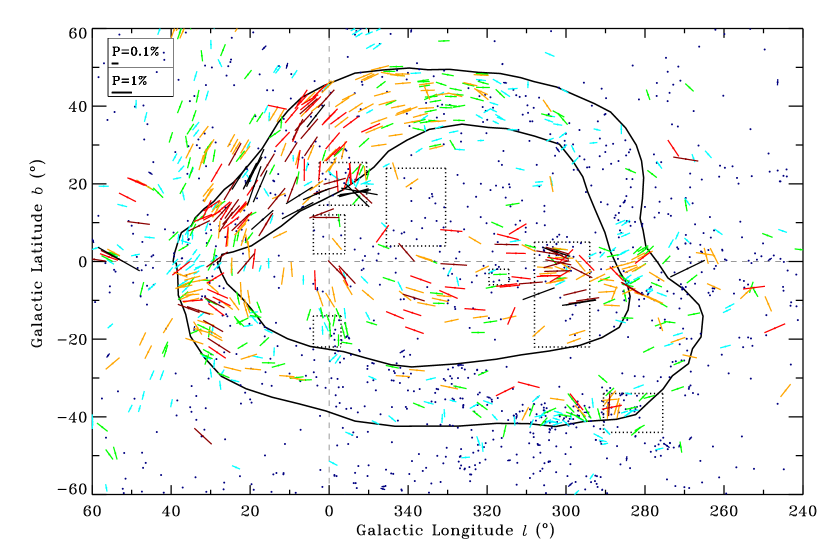
Figure 5: Distribution of polarization vectors along the studied region. The thick contour corresponds to the annular feature proposed by Egger & Aschenbach (1995) and the dotted rectangles indicate the locations of the main dark clouds distributed along this region, as shown in Figure 1. To improve visualization, the sizes of the $P$-vectors are plotted proportionally to $\sqrt{P}$, and a grayscale scheme (colored at the electronic version) was used (as specified on Table 2).

The model that suggests the existence of a dense and neutral “wall” of interstellar material between the LC and Loop I claims that the supposed interaction ring would be located at a distance of approximately $70$ pc, corresponding to a $N_{\mathrm{HI}}$ transition from $\sim 10^{20}$ cm^-2 to $\sim 7\times 10^{20}\$cm^-2 (Egger & Aschenbach, 1995). In this case, the standard gas-to-dust ratio proposed by Knude (1978) may be used to interpret this transition as a rise in $E(b-y)$ from $\approx 0\fm 015$ to $\approx 0\fm 100$, which corresponds to maximum value of polarization ($P_{max}$) increasing from $\approx 0.2$ to $\approx 1.3\%$.

Table 2: Color/Grayscale scheme used in the polarization analysis

$P(\%)$	Color	Grayscale	$E(b-y)_{min}$
$\leq 0.1$	navy blue	black	$\leq 0\fm 008$
$0.1-0.3$	cyan	light gray	$\approx 0\fm 008-0\fm 025$
$0.3-0.5$	green	light gray	$\approx 0\fm 025-0\fm 040$
$0.5-0.9$	orange	light gray	$\approx 0\fm 040-0\fm 070$
$\mathbf{0.9-1.3}$	red	dark gray	$\mathbf{\approx 0\fm 070-0\fm 100}$
$1.3-2.0$	dark red	black	$\approx 0\fm 100-0\fm 160$
$>2.0$	black	black	$>0\fm 160$

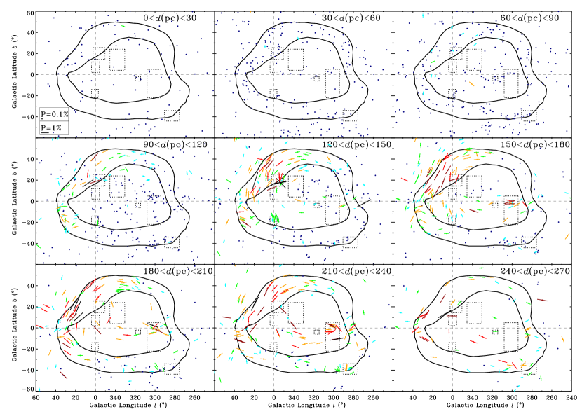
Figure 6: Distribution of polarization vectors along the interface region, divided by distance intervals of $30$ pc each. Notice the existence of dark gray vectors (colored in red at the electronic version, corresponding to the transition to $P\approx 0.9-1.3\%$) on the left side at about $90-120$pc (the loop-shaped polarization feature in the direction of $(l,b)\approx(0^{\circ},30^{\circ})$), whereas on the right side they are not clearly seen before $240$pc. The details are the same as in Figure 5.

Knude (1978) asserts that stars with $E(b-y)\geq 0\fm 030$ must be located behind at least a diffuse interstellar cloud. Hence, if $E(b-y)\sim 0\fm 070$, the objects are probably reddened by a denser interstellar cloud, which might as well polarize the stellar light. Based on this reasoning, in the following polarization analysis we shall look for a transition from $P_{max}\approx 0.2\%$ to $P_{max}\approx 0.9-1.3\%$, which corresponds to $E(b-y)$ going from $0\fm 015$ to $0\fm 070-0\fm 100$. In principle, this is the expected transition if the proposed HI column density for the ring is considered. To ease the comparison between the polarization and the color excess we will adopt a criterion similar to Reis & Corradi (2008), for the typical values of $E(b-y)$ corresponding to the ring transition.

The distribution of polarization vectors along the entire studied region is shown on Figure 5, where lines represent the $\mathbf{\bf{E}}$-vectors of the partially polarized light, centered on the position of each star. We have chosen to represent the size of each vector proportional to $\sqrt{P}$, hence allowing a better visualization of the polarization pattern, since most of the objects show low polarization degree ($\leq 0.5\%$). For polarized stars ($P\geq 0.1\%$), only those satisfying $\Delta P/P<0.2$ and $\Delta\theta_{gal}<20^{\circ}$ are plotted, eliminating 338 objects from this kind of diagram. The $\Delta\theta_{gal}<20^{\circ}$ requirement implies that objects with large uncertainties on polarization angle will not be plotted. Considering the typical polarization degree error of $\sim 0.05\%$, we define objects with $P\leq 0.1\%$ as “unpolarized”, based on our instrumental precision. These objects are represented as a single dot.

Moreover, in order to further improve the visualization, a color scheme corresponding to polarization degree intervals was adopted. Table 2 specifies the colors and grayscales corresponding to each polarization interval, as well as the minimum color excess value ($E(b-y)_{min}$) associated to each $P$ (assuming that the relation discussed on section 3 is valid). Notice that the dark gray level (i.e., the red color at the electronic version) corresponds to the transition of $0.9-1.3\%$.

To analyze the distribution of the polarization vectors as a function of distance, the same diagram of Figure 5 was sliced in distance intervals of $30$ pc each. These plots are shown on Figure 6, from $0$ to $270$ pc. Regions that are closer to the Sun (up to $60$ pc) exhibit mainly unpolarized stars ($P<0.1\%$), consistent with the presence of the LC. The first weakly polarized stars (with $P<0.5$%) are distributed along the western (left) side ($l>330^{\circ}$) of the interaction region in the $60-90$ pc interval. The first large-scale interstellar structure is observed in the $90-120$ pc interval near $(l,b)\approx(0^{\circ},30^{\circ})$, where the polarization vectors run parallel to the ring contour and show high polarization degree ($P>1.3\%$) along most lines-of-sight, forming something like a “loop” pattern. Notice that up to this distance range, the eastern (right) side ($l\approx 290^{\circ}$) is still composed mainly by unpolarized stars.

The main dark clouds located inside the ring contour are located along the $120-150$ pc and $150-180$ pc distance intervals, e.g.: R CrA ($l,b\approx 0^{\circ},-18^{\circ}$), $\rho$ Oph ($l,b\approx 355^{\circ},+20^{\circ}$) and the Southern Coalsack/Chamaeleon/Musca complex ($l,b\approx 300^{\circ},-10^{\circ}$). Notice that the large-scale structure observed along the left side of the ring shows polarization vectors distributed roughly parallel to the ring contour orientation. The first few weakly polarized stars ($P<0.3$%) appear at the south-right side ($280^{\circ}<l<320^{\circ}$,$-50^{\circ}<b<-20^{\circ}$) in the $150-180$ pc interval. However, the majority of the objects in this region are still unpolarized.

The $180-210$ pc and $210-240$ pc diagrams show that the first stars located along the right side of the ring presenting slightly higher polarization degree ($P>0.5$%) appear only after $200$pc. Also notice that the polarization vectors along this direction are perpendicular to the ring structure, in contrast to the situation observed at the left side, where the vectors run parallel to the ring contour.

The $240-270$ pc diagram shows that up to $270$ pc the right region is composed predominantly by stars with polarization in the range $0-0.9$%. Some stars possess $P>0.9\%$ suggesting that the expected transition to $P\sim 0.9-1.3\%$ might occur along this distance range. For higher distances, the sample becomes non-uniform and incomplete, an expected effect, given the rapid decrease in the number of observed stars beyond $250$pc, as can be seen from Figure 2a.

5 Polarization as a function of distance at the interface region

Several interstellar structures are distributed along the interface with the Loop I superbubble, and can be identified by a rise in the $P(\%)$ values when such a feature is crossed. To build a better picture of the distances to each individual structure along the whole region, we have plotted diagrams of $P(\%)$ as a function of distance $d$(pc) to several rectangular areas positioned along the entire surveyed area. These diagrams are limited to the range $0\%<P<2\%$ to offer a better view of the smaller $P$ variations.

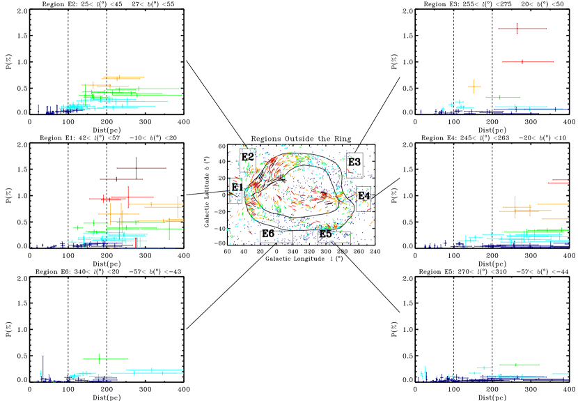
Figure 7: Diagrams of $P(\%)\times distance(pc)$ for rectangular regions outside the ring, as indicated in the central panel. Polarization vectors are also plotted along the interface region at the center, as in Figure 5. A rise to $P\approx 0.6$% is observed at approximately $130-140$ pc along E1 and E2 areas, coinciding to the direction of the NPS. These diagrams are limited to the range $0\%<P<2\%$.

Our analysis was divided between three regions: outside (E1-E6, Figure 7), along (A1-A12, Figure 8), and inside (I1-I6, Figure 9) the annular ring-like feature proposed by Egger & Aschenbach (1995). This scheme shall allow us to study specifically the structure of the supposed ring and its relation to the surroundings, as well as to compare our results with the previous photometric analysis by Reis & Corradi (2008). The limiting Galactic coordinates of each rectangular region are indicated in the corresponding figures.

5.1 Regions outside the ring

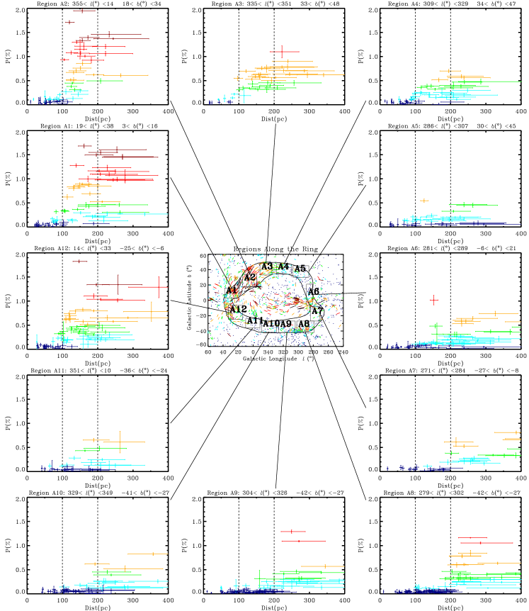
Figure 8: Diagrams of $P(\%)\times distance(pc)$ for rectangular regions along the ring. The $0.9-1.3\%$ transition occurs at $\approx 100$ pc on the left side (e.g., A2 area) and is not clearly identified before $\approx 250$ pc on the right side region (e.g., A8 area). These diagrams are limited to the range $0\%<P<2\%$.

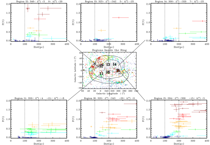
Figure 9: Diagrams of $P(\%)\times distance(pc)$ for rectangular regions inside the ring. A rise in P(%) is seen at $\approx 120-130$ pc in the directions of R CrA (region I1, $P_{max}\approx 0.6\%$) and $\rho$ Oph (region I2, $P_{max}>2\%$). The complex of dark clouds defined by the Southern Coalsack, Chamaeleon, and Musca (I5 region) displays a sharp rise to $P>2\%$ at approximately $150-180$ pc. These diagrams are limited to the range $0\%<P<2\%$.

For the regions outside the ring area (Figure 7), interstellar polarization is mainly $\leq 0.3$% up to approximately $200$pc in almost all directions, although more data would be necessary to carry out an adequate analysis.

Exceptions are observed at E1 and E2 regions, where a rise to $P\approx 0.6$% is observed at approximately $130-140$ pc. These regions coincide with the direction of the “North Polar Spur” (NPS), the brightest rim of Loop I, well-known to be a large radio filament, which extends to the north along $30^{\circ}$ in longitude. The rise in $P(\%)$ is consistent with the presence of this structure.

5.2 Regions along the ring

A sharp rise in $P$ (in some cases higher than $1.3\%$) is observed for several areas along the left side of the interaction region (areas A1, A2, A3, and A12 of Figure 8) indicating that the interstellar structures are positioned at a distance of $\approx 80-100$pc in these directions. These areas coincide with the large loop pattern identified by analyzing the polarization vectors, as discussed on Section 4 (see, for example, Figures 5 and 6). Some dark clouds and dense structures are known to be present in these directions, particularly: Sag-South and Aql-South ($27^{\circ}<l<40^{\circ}$; $-21^{\circ}<b<-10^{\circ}$), the Scutum dark cloud ($l=25^{\circ}$;$b=1^{\circ}$), the Oph-Sgr molecular clouds ($8^{\circ}<l<40^{\circ}$; $9^{\circ}<b<24^{\circ}$) etc.

Carrying on the analysis in the left-right direction, a smooth decrease to $P\approx 0.5\%$ is observed at the northern (e.g., A4 and A5) and southern areas (e.g., A10 and A11) at $\sim 100$ pc, when compared to polarization values at the same distance on the left areas (e.g., A1, A2, and A12).

In the regions to the right, the first clear rise to $P\approx 0.6\%$ occurs at $180-200$ pc along the A6, A7 and A8 areas. However, the expected $0.9-1.3\%$ transition is not clearly seen before $\sim 250$ pc (see A8 and A9 areas). Specifically, part of the A8 region coincides with a diffuse interstellar filament in the direction of the Mensa constellation, with an estimated distance of $d=230\pm 30$ pc (Penprase et al., 1998).

Some regions (e.g., the A5 region) show low polarization values ($P<0.5\%$) up to $\sim 300$ pc, suggesting that the structure is discontinuous and probably highly fragmented.

5.3 Regions inside the ring

The regions inside the ring area (Figure 9) are marked by the presence of several well-known dark clouds distributed relatively close to the GP along the southern sky (see e.g., Dame et al., 2001).

The diagrams related to left areas exhibit a rise in P(%) at $\approx 120-130$ pc in the directions of R CrA (region I1, $P_{max}\approx 0.6\%$) and $\rho$ Oph (region I2, $P_{max}>2\%$). The I2 area also encompasses the region of the Pipe Nebula, which is located at a distance of $145\pm 16$ pc from the Sun (Alves & Franco, 2007).

Along the I3 and I4 regions our data are quite sparse and do not lead us to any clear conclusion, although there seems to be a trend to low polarization values ($P<0.6\%$) up to $\approx 200$ pc. The complex of dark clouds defined by the Southern Coalsack, Chamaeleon, and Musca (SCCM, I5 region) displays a sharp rise to $P>2\%$ at approximately $150-180$ pc. This distance corroborates previous photometric analysis by Corradi et al. (1997); Corradi et al. (2004). A smooth rise from $P<0.1\%$ (up to $\sim 100$ pc) to $P\approx 1.3\%$ (at $\sim 200$ pc) is observed at the I6 area.

6 Discussion

6.1 Summary of polarimetric properties between regions outside, along and inside the ring

Table 3: Summary of the analysis of rectangular areas outside, along, and inside the ring

Area	$(l_{min},l_{max})$	$(b_{min},b_{max})$	Comment
E1	$(42^{\circ},57^{\circ})$	$(-10^{\circ},20^{\circ})$	Orientation along the NPS; $P$ rise to $\approx 0.6$% at $130-140$ pc
E2	$(25^{\circ},45^{\circ})$	$(27^{\circ},55^{\circ})$	Same as E1; Northern portion of the NPS loop
E3	$(255^{\circ},275^{\circ})$	$(20^{\circ},50^{\circ})$	Low $P$ ($\leq 0.3$%) up to approximately $200$ pc
E4	$(245^{\circ},263^{\circ})$	$(-20^{\circ},10^{\circ})$	Same as E3
E5	$(270^{\circ},310^{\circ})$	$(-57^{\circ},-44^{\circ})$	Same as E3
E6	$(340^{\circ},20^{\circ})$	$(-57^{\circ},-43^{\circ})$	Same as E3
A1	$(19^{\circ},38^{\circ})$	$(3^{\circ},16^{\circ})$	$P$ rise to $\approx 0.7$% at $80-100$ pc; loop pattern; Serpens-Aquila cloud
A2	$(355^{\circ},14^{\circ})$	$(18^{\circ},34^{\circ})$	$P$ rise to $>1.0$% at $\approx 100$ pc; loop pattern orientation
A3	$(335^{\circ},351^{\circ})$	$(33^{\circ},48^{\circ})$	$P$ rise to $\approx 0.7$% at $\approx 100$ pc; $P$ decrease compared to A1 and A2
A4	$(309^{\circ},329^{\circ})$	$(34^{\circ},47^{\circ})$	Same as A3; final portion of the polarization loop pattern
A5	$(286^{\circ},307^{\circ})$	$(30^{\circ},45^{\circ})$	Low $P$ values ($<0.5\%$) up to $\sim 300$ pc
A6	$(281^{\circ},289^{\circ})$	$(-6^{\circ},21^{\circ})$	Orientation parallel to the GP; $P$ rise to $0.6$% at $\approx 180-200$ pc
A7	$(271^{\circ},284^{\circ})$	$(-27^{\circ},-8^{\circ})$	$P$ rise to $0.6$% at $\approx 180-200$ pc
A8	$(279^{\circ},302^{\circ})$	$(-42^{\circ},-27^{\circ})$	$P=0.9-1.3\%$ at $\sim 250$ pc; interstellar filament at $d=230\pm 30$ pc
A9	$(304^{\circ},326^{\circ})$	$(-42^{\circ},-27^{\circ})$	$P=0.9-1.3\%$ transition at $\sim 250$ pc
A10	$(329^{\circ},349^{\circ})$	$(-41^{\circ},-27^{\circ})$	$P$ rise to $0.6$% at $\approx 180-200$ pc
A11	$(351^{\circ},10^{\circ})$	$(-36^{\circ},-24^{\circ})$	$P$ rise to $0.6$% at $\approx 150$ pc; $P$ decrease compared to A12
A12	$(14^{\circ},33^{\circ})$	$(-25^{\circ},-6^{\circ})$	$P$ rise to $\approx 0.7$% at $80-100$ pc;
I1	$(350^{\circ},4^{\circ})$	$(-21^{\circ},-8^{\circ})$	R CrA dark cloud; rise to $P\approx 0.6\%$ at $\approx 120-130$
I2	$(346^{\circ},5^{\circ})$	$(0^{\circ},20^{\circ})$	$\rho$ Oph and Pipe Nebula dark clouds; rise to $P>2\%$ at $\approx 120-130$
I3	$(325^{\circ},342^{\circ})$	$(5^{\circ},25^{\circ})$	Low $P$ ($<0.6\%$) up to $\approx 200$ pc; few data
I4	$(300^{\circ},320^{\circ})$	$(7^{\circ},25^{\circ})$	Same as I3
I5	$(294^{\circ},309^{\circ})$	$(-15^{\circ},5^{\circ})$	SCCM dark clouds; rise to $P>2\%$ at $\approx 150-180$ pc
I6	$(320^{\circ},343^{\circ})$	$(-20^{\circ},0^{\circ})$	Smooth rise from $P<0.1\%$ (at $\sim 100$ pc) to $P\approx 1.3\%$ (at $\sim 200$ pc)

The main polarimetric properties exposed in sections 4 and 5, associated to each of the rectangular areas inside, along and outside the ring contour are summarized in table 3.

Inside the contour, large polarization values ($P>2\%$) are seen in the direction of several dark clouds distributed along the interface area. When analyzing the distances to these interstellar structures, we notice a difference in positions of clouds from the left side (R CrA, $\rho$ Oph; at $120-130$ pc) when compared to the right side (Southern Coalsack, Chamaeleon and Musca complex; at $150-180$ pc). This may indicate that the interface is tilted with respect to the Sun.

Figure 5 show that inside the contour the polarized vectors’ orientation is mainly parallel to the GP. However, along the left side (particularly along the R CrA dark cloud), vectors are oriented perpendicularly to the GP. According to Harju et al. (1993), an expanding shell from the Upper Centaurus-Lupus (UCL) Sco-Cen sub-group would have collided with the R CrA dark cloud a few million years ago, creating the cloud’s cometary shape and triggering star formation. In this direction, polarized vectors are oriented parallel to the “head-tail” direction of the cloud, and therefore perpendicular to the GP. This could be a local effect of the distortion of magnetic field lines due to the passage of the expanding shell.

Along the contour of the ring, a coherent alignment of polarization vectors appears toward the left-northern side (areas A1, A2, A3 and A4), tracing a loop-shaped structure of magnetic field lines. The distance to this structure is evident from a rise in polarization values at $80-100$ pc. The Serpens-Aquila molecular cloud ($l\approx 30^{\circ},b\approx 4^{\circ})$, which is positioned toward the A1 area, is probably located at $200$ pc, according to Dame et al. (1987, 2001). In fact, the A1 diagram shows a second polarization rise at $\sim 200$ pc, which could correspond to this interstellar structure. However, the first rise to $P\approx 0.6\%$ at $\sim 100$ pc (also detected at the photometric survey) suggests the presence of nearer interstellar material in front of the denser molecular cloud.

Along the right side of the ring, the first rise to low polarization values $\sim 0.5\%$ occurs only after $200$ pc. Furthermore, the vectors’ orientation is mainly uncorrelated to the contour of the ring. Further discussion of vectors’ orientation along the ring will be presented in section 6.3

Outside the contour of the ring the most conspicuous structure is the North Polar Spur (along E1 and E2 areas), located at approximately $130-140$ pc. In this direction polarized vectors are oriented in a loop pattern parallel to the radio filament.

6.2 Comparison with the color excess analysis

The results presented in section 5 are in agreement with a similar analysis made by Reis & Corradi (2008) using $E(b-y)$ color excesses as a function of distance to several rectangular areas located along the interface region. Particularly, the above mentioned work revealed that the expected transition to $E(b-y)\approx 0\fm 070-0\fm 100$, corresponding to the ring’s column density, occurs on the left side of the ring at $d=110\pm 20$ pc, while the right side transition is not clearly seen before $d=280\pm 50$ pc. Accordingly, our data show that the left side rise to $P\sim 0.9-1.3\%$ occurs at $\approx 100$ pc, while the right side regions exhibit the same transition only beyond $\approx 250$ pc.

The results of both surveys also match for areas inside and outside the ring region. When comparing the polarimetric and photometric analysis along each line-of-sight, the increase in polarization and $E(b-y)$ always occur at the same distances. For example, if we compare Figures 9, 10 and 11 from Reis & Corradi (2008) with our Figures 7, 8 and 9, we note that: in the direction of A2, a rise both in polarization and $E(b-y)$ is seen at approximately $100$ pc; toward the SCCM clouds (I5 area), both $P$ and $E(b-y)$ increases sharply at $150-180$ pc. Such correlations may be noted throughout several other areas and may be explained by the good association between color excesses and polarization values, as presented on section 3.

Despite the correlation between $P$ and $E(b-y)$, polarization efficiency variations along the ring possibly could exist locally, toward specific areas, particularly in the direction of star-forming regions, where the radiation field is more intense (Andersson & Potter, 2007). However, given the largely correlated distances obtained from the polarimetric analysis when compared to the photometric survey (Reis & Corradi, 2008), local variations of $P/A_{V}$ does not affect our global conclusions on the positions of the several interstellar structures.

Comparing the polarization properties between the interfaces’s left and right sides, it is worth noting that the gradual decrease in the highest polarization values observed in the right side ($P\approx 2\%$) relative to the left ones ($P\approx 0.9\%$) may be due to a greater proximity of the right side with the “magnetic pole” associated to the large-scale structure of the Galactic magnetic field at the solar neighborhood, which is mainly directed along the local spiral arm of the Galaxy. According to Whittet (2003) and Heiles & Crutcher (2005) the magnetic pole is located toward $(l,b)=(260^{\circ},0^{\circ})$, and can be viewed face-on in this direction. This is revealed by a greater dispersion in polarization angles and lower polarization degree values toward this line-of-sight, which traces only the sky-projected component of the magnetic field. However, this fact doesn’t impair our analysis of polarization as a function of distance toward the right side regions, since the same results are observed with the color excess analysis (which does not depend on the magnetic field configuration), revealing similar distances to the interstellar structures.

These evidence confirm the distorted nature of the large-scale interface of the interstellar medium in the direction of Loop I. Besides, by analyzing specifically the A5 and A11 areas along the ring, we note a lower dust column density along these lines-of-sight (see Figures 5 and 8) which may be an indication of fragmentation of the suggested large-scale ring structure, or simply that such ring feature may not exist.

6.3 Analysis of the polarization vectors’ direction and its relation to the ring structure

The analysis of the polarization vectors orientation for different distance bands (Figure 6), reveals that on the $180-210$ pc and $210-240$ pc diagrams the polarization vectors along the right side direction do not present correlation with the ring contour orientation, in contrast to the situation observed at the left side, where the vectors run parallel to the ring contour. This relation between polarization vectors’ mean direction and the direction of the ring contour is further investigated on Figure 10, where we show histograms of the polarization angle ($\theta_{gal}$) to the same previously studied rectangular areas. These histograms only account for the polarized stars, i.e., with $P>0.1\%$ and $\Delta P/P<0.2$. The dashed lines on the histograms indicate the direction of the ring contour along each studied area.

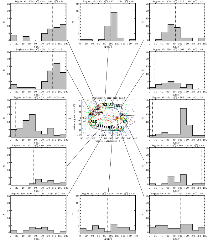
Figure 10: Histograms of polarization vectors’ direction to the same rectangular areas analyzed in Figure 8. The dashed lines on the histograms roughly indicate the direction of the contour along each specific area. Polarization vectors are also plotted along the interface region at the center, as in Figure 5. Note that left and northern areas (e.g., A1, A2, A3, and A4) show predominant vectors’ orientation parallel to the ring contour (dashed lines), while at the right side and southern areas (e.g., A6, A7, A8, and A9) the main vectors’ directions show no relation to the ring contour direction.

In fact, the histograms associated to the left-northern areas (e.g., A1-A4) show a good correlation between the ring contour direction and the main values of polarization direction, as indicated by the coincidence of the histogram peak and the dashed line, that indicates the ring contour orientation.

Iwan (1980), de Geus (1992), and Heiles (1998) pointed out that these lines-of-sight intercept several spherical “shells” of interstellar material which are centered on the sub-groups of Sco-Cen and are most probably generated by stellar wind and SN explosion from these massive stars. Furthermore, by analyzing the radio continuum maps ($408$MHz) by Haslam et al. (1982) and the relation between the shells’ direction and the polarization vectors, Heiles (1998) proposed that this configuration could be created due to the distortion of the local magnetic field along constant “longitude” lines on the surface of the expanding shells.

In contrast, histograms related to the right side areas (e.g., A6 and A7) show that the predominant polarization direction is mainly uncorrelated to the ring contour direction, as indicated by the different position of the dashed line and the peak of the histogram. Furthermore, the southern areas (A8, A9, and A10) show a large polarization vectors dispersion, as suggested by the flat shape of the histogram.

This could be related to the low polarization sky-projected component of the local magnetic field (being viewed face-on) or perhaps due to the presence of several interstellar sub-structures. In fact, Penprase et al. (1998) reported the existence of a diffuse interstellar filament located in the direction of the A8 area at $d=230\pm 30$ pc. A more detailed analysis of the polarization vectors in the direction of this filament suggest a clear relation with the morphology of such feature, with the polarization vectors positioned perpendicular to the direction of the filament.

These results show that the behavior of the magnetic field direction in relation to the direction of the ring contour is markedly different between the left and right side regions.

6.4 Implications on the models of the Local ISM

The existence (or not) of the interaction ring is closely related to the true nature of the LC. Several models attempting to explain the origin of the LC have been proposed, and have been divided here in three main classes, as discussed below.

On one side, the first class claims that the LC may have been created due to one or more SN explosions at the solar neighborhood a few million years ago, which would have swept the local neutral material and heated the interstellar gas up to $10^{6}$K (Cox & Smith, 1974; Cox & Anderson, 1982; Cox & Reynolds, 1987; Gehrels & Chen, 1993; Smith & Cox, 2001; Maíz-Apellániz, 2001; Berghöfer & Breitschwerdt, 2002; Fuchs et al., 2006). The hot gas would have generated a local component on the all-sky observed soft X-ray emission (corresponding to the “Hot Local Bubble”). In fact, using data from the ROSAT survey ($0.25$keV) and assuming a constant emissivity of the plasma, Snowden et al. (1990) and Snowden (1998) attempted to produce tridimensional maps of the Hot Local Bubble.

On the other side, a second class of models suggest that the LC would be a part of the nearby Loop I superbubble, in a sense that different star forming epochs from the Sco-Cen OB association would have created different shock fronts, which expanded asymmetrically in the direction of the Sun, i.e., a low density region between the Galaxy’s spiral arms (Frisch, 1981; Frisch & York, 1983; Frisch, 1995; Wolleben, 2007). Frisch (2008, 2010) argues further that this model is consistent with the view that two separate synchrotron emitting interstellar shells centered on different parts over the Sco-Cen association can reproduce large-scale structures revealed by recent radio polarization surveys, as proposed by Wolleben (2007). Furthermore, the existence of a global flux of interstellar material at the solar neighborhood toward the opposite direction of Loop I (Lallement et al., 1995; Lallement, 1998; Cox & Helenius, 2003), i.e., toward $(l,b)\approx(186^{\circ},-16^{\circ})$, supports the idea that some recent event may have caused the large-scale movement of the interstellar material driven away from Sco-Cen.

A third class of models propose that the Local Cavity is not really a bubble in a sense that its origin is not associated to SN explosions, being actually an ordinary cavity (the “local void”) in the local interstellar medium (Bruhweiler, 1996; Mebold et al., 1998). The local cavity would be a low-density volume of space defined by several interacting shells, like Loops I, II, III, and IV, the Gum Nebula, the Orion-Eridanus Superbubble, among others.

If the interaction ring really exists, the first class of models provides a suitable scenario, since the collisional models by Yoshioka & Ikeuchi (1990) would require both bubbles (Local and Loop I) to be expanding, and in addition, at least one of them should have reached the radiative stage of evolution prior to the interaction in order to generate the proposed annular dense region, as pointed out by Egger & Aschenbach (1995).

However, some issues have been recently presented regarding the idea that the LC would have been created by such supernovae explosions. Specifically, recent studies revealed that a major part of the observed soft X-ray emission could be related to a much closer component, associated to the solar wind charge exchange effect at the heliosphere, which have not been properly accounted on the previous analysis (Cravens, 1997; Freyberg, 1998; Cox, 1998; Cravens, 2000; Robertson et al., 2001; Robertson & Cravens, 2003; Lallement, 2004; Welsh & Shelton, 2009).

Our data demonstrates that the classical concept of a unique bounding ring at the interaction area is misleading, in view of the largely discrepant distances between the different parts of the annular area, and also due to the widely different behavior of the magnetic field lines along the structure, which suggest that the left and right sides of the proposed ring are possibly uncorrelated. Figure 3 from the work by Breitschwerdt et al. (1996) shows a conceptual representation of the classical model attributed to the interaction ring.

Instead of the scenario proposed by Egger & Aschenbach (1995), our data suggest that this structure is quite distorted and fragmented, unlike one would expect from a unique feature. However, this evidence does not refute the first class of models, it simply adds a new constraint to computational simulations which attempts to reproduce the characteristics of the LC and Loop I through SN energy input. Therefore, these models should account for the shape of the magnetic field lines, and reproduce the observed distortion along the interface area.

On the other hand, the second and third types of model do not require the existence of an interaction ring, since the occurrence of SN explosions inside the LC are not considered. Particularly, the model provided by Wolleben (2007) allow the shape of magnetic field lines to be tested by using polarimetric data, similar to what has been accomplished by Frisch (2008, 2010). According to this scenery, Loop I is conceived as consisting of two synchrotron-emitting shells (namely S1 and S2), that reproduces the large-scale magnetic field structure as revealed by polarimetric radio continuum surveys. As an illustration of this model, Figure 11 shows the projected positions of both shells along with the optical polarimetric data distribution from this work.

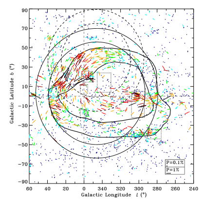
Figure 11: Distribution of polarimetric data in the direction of Loop I, used to illustrate the Wolleben (2007) model, represented by the projected positions of the S1 (solid line) and S2 (dashed line) shells. We have also included the contour of the ring proposed by Egger & Aschenbach (1995), and the positions of several dark clouds located along the interface with Loop I.

From the point of view of our results, the advantage of such model is that it doesn’t require the existence of an interaction ring between the LC and Loop I. However, it is important to point out that, referring to Figure 11, it is possibly misleading to perform a direct comparison of the shells’ positions with the vectors direction. Instead, a valid analysis would demand a rigorous comparison between the polarization vectors and the summed projected magnetic field lines, derived by Wolleben (2007), along all distances and directions. This means that the interweaving magnetic field lines related to the S1 and S2 shells should be projected in the plane-of-sky and thereafter vectorially summed along each line-of-sight, similar to what has been discussed at the Appendix from Wolleben (2007) (where the integrated Q and U Stokes parameters were computed based on the magnetic field structure).

Although there exist some correlations of the polarization vectors’ direction with respect to the shells’ positions (especially toward E1 and E2 areas $-$ the North Polar Spur $-$ when compared to the left side of the S2 shell), such effect may be possible only when the projected magnetic field follows the direction of the shell’s border, which is not true in general, considering the projections and the combined effect of both shells. Therefore, it is soon to assert if this is an adequate model, and it would also be expected to reproduce the observed gas and dust column densities in the lines-of-sight of the Loop I shells.

7 Conclusions

We have carried out a polarimetric survey of $878$ Hipparcos stars in the general direction of the Loop I superbubble’s interface with the LC. Our sample was complemented with the data from Heiles (2000) catalogue. The main results of the analysis are summarized below:

• Along the ring structure proposed by Egger & Aschenbach (1995), the left side rise from $P\sim 0.2\%$ to $P\sim 0.9-1.3\%$, which correspond to the ring’s column density, occurs at $\approx 100$ pc, while at the right side regions the same transition occurs only beyond $\approx 250$ pc. This trend corroborates the color excess analysis by Reis & Corradi (2008);

• A gradual decrease in the polarization values is observed in the left-right direction along the contour of the interaction ring;

• The analysis of the polarization vectors direction along the interface revealed that along the right side the predominant direction of the vectors do not present correlation with the direction of the ring contour, in contrast to the situation observed at the left side, where the vectors run parallel to the ring structure.

Altogether, these evidence confirm the distorted nature of the interstellar interface between the LC and Loop I. The low polarization values toward some areas along the interaction ring suggest that, if it really exists, it is probably highly fragmented and twisted. However, the configuration of the sky-projected component of magnetic field in relation to the direction of the ring contour reveals markedly different behavior in the left and right sides. This fact casts some doubt on the existence of the ring-like structure as a unique large-scale feature.

Our methods were mainly the analysis based on the distances to the interstellar structures and the shape of magnetic field lines along the interface. These studies were used in a qualitative comparison with the existent models for the local interstellar medium. The existence (or not) of the ring is closely related to the true nature and associated origin models of the Local Cavity, and shall deserve a particularly special attention.

References

- Alves & Franco (2007) Alves, F. O., & Franco, G. A. P. 2007, A&A, 470, 597
- Andersson & Potter (2007) Andersson, B.-G., & Potter, S. B. 2007, ApJ, 665, 369
- Bailey & Hough (1982) Bailey, J., & Hough, J. H. 1982, PASP, 94, 618
- Bastien et al. (1988) Bastien, P., Drissen, L., Menard, F., Moffat, A. F. J., Robert, C., & St-Louis, N. 1988, AJ, 95, 900
- Beck (2001) Beck, R. 2001, Space Sci. Rev., 99, 243
- Beck (2002) Beck, R. 2002, Disks of Galaxies: Kinematics, Dynamics and Perturbations, 275, 331 OPD
- Berghöfer & Breitschwerdt (2002) Berghöfer, T. W., & Breitschwerdt, D. 2002, A&A, 390, 299
- Berkhuijsen et al. (1971) Berkhuijsen, E. M., Haslam, C. G. T., & Salter, C. J. 1971, A&A, 14, 252
- Breitschwerdt et al. (1996) Breitschwerdt, D., Egger, R., Freyberg, M. J., Frisch, P. C., & Vallerga, J. V. 1996, Space Sci. Rev., 78, 183
- Breitschwerdt et al. (2000) Breitschwerdt, D., Freyberg, M. J., & Egger, R. 2000, A&A, 361, 303
- Blaauw (1964) Blaauw, A. 1964, The Galaxy and the Magellanic Clouds, 20, 50
- Bruhweiler (1996) Bruhweiler, F. C. 1996, IAU Colloq. 152: Astrophysics in the Extreme Ultraviolet, 261
- Centurion & Vladilo (1991) Centurion, M., & Vladilo, G. 1991, ApJ, 372, 494
- Codina-Landaberry & Magalhaes (1976) Codina-Landaberry, S., & Magalhaes, A. M. 1976, A&A, 49, 407
- Corradi et al. (1997) Corradi, W. J. B., Franco, G. A. P., & Knude, J. 1997, A&A, 326, 1215
- Corradi et al. (2004) Corradi, W. J. B., Franco, G. A. P., & Knude, J. 2004, MNRAS, 347, 1065
- Cox & Smith (1974) Cox, D. P., & Smith, B. W. 1974, ApJ, 189, L105
- Cox & Anderson (1982) Cox, D. P., & Anderson, P. R. 1982, ApJ, 253, 268
- Cox & Reynolds (1987) Cox, D. P., & Reynolds, R. J. 1987, ARA&A, 25, 303
- Cox (1998) Cox, D. P. 1998, IAU Colloq. 166: The Local Bubble and Beyond, 506, 121
- Cox & Helenius (2003) Cox, D. P., & Helenius, L. 2003, ApJ, 583, 205
- Cravens (1997) Cravens, T. E. 1997, Geophys. Res. Lett., 24, 105
- Cravens (2000) Cravens, T. E. 2000, ApJ, 532, L153
- Dame et al. (1987) Dame, T. M., et al. 1987, ApJ, 322, 706
- Dame et al. (2001) Dame, T. M., Hartmann, D., & Thaddeus, P. 2001, ApJ, 547, 792
- Davis & Greenstein (1951) Davis, L. J., & Greenstein, J. L. 1951, ApJ, 114, 206
- Draine & Weingartner (1996) Draine, B. T., & Weingartner, J. C. 1996, ApJ, 470, 551
- Draine & Weingartner (1997) Draine, B. T., & Weingartner, J. C. 1997, ApJ, 480, 633
- Egger & Aschenbach (1995) Egger, R. J., & Aschenbach, B. 1995, A&A, 294, L25
- ESA (1997) ESA, 1997, The Hipparcos and Tycho Catalogues, ESA SP-1200. ESA Publications Division, Noordwijk
- Fosalba et al. (2002) Fosalba, P., Lazarian, A., Prunet, S., & Tauber, J. A. 2002, ApJ, 564, 762
- Franco (1990) Franco, G. A. P. 1990, A&A, 227, 499
- Freyberg (1998) Freyberg, M. J. 1998, IAU Colloq. 166: The Local Bubble and Beyond, 506, 113
- Frisch (1981) Frisch, P. C. 1981, Nature, 293, 377
- Frisch & York (1983) Frisch, P. C., & York, D. G. 1983, ApJ, 271, L59
- Frisch (1995) Frisch, P. C. 1995, Space Sci. Rev., 72, 499
- Frisch (2007) Frisch, P. C. 2007, Space Sci. Rev., 130, 355
- Frisch (2008) Frisch, P. C. 2008a, Space Sci. Rev., 142
- Frisch (2010) Frisch, P. C. 2010, ApJ, 714, 1679
- Fruscione et al. (1994) Fruscione, A., Hawkins, I., Jelinsky, P., & Wiercigroch, A. 1994, ApJS, 94, 127
- Fuchs et al. (2006) Fuchs, B., Breitschwerdt, D., de Avillez, M. A., Dettbarn, C., & Flynn, C. 2006, MNRAS, 373, 993
- de Geus (1992) de Geus, E. J. 1992, A&A, 262, 258
- Gil-Hutton & Benavidez (2003) Gil-Hutton, R., & Benavidez, P. 2003, MNRAS, 345, 97
- Gehrels & Chen (1993) Gehrels, N., & Chen, W. 1993, Nature, 361, 706
- Hall (1949) Hall, J. S. 1949, Science, 109, 166
- Harju et al. (1993) Harju, J., Haikala, L. K., Mattila, K., Mauersberger, R., Booth, R. S., & Nordh, H. L. 1993, A&A, 278, 569
- Haslam et al. (1982) Haslam, C. G. T., Salter, C. J., Stoffel, H., & Wilson, W. E. 1982, A&AS, 47, 1
- Heiles (1998) Heiles, C. 1998, IAU Colloq. 166: The Local Bubble and Beyond, 506, 229
- Heiles (2000) Heiles, C. 2000, AJ, 119, 923
- Heiles & Crutcher (2005) Heiles, C., & Crutcher, R. 2005, Cosmic Magnetic Fields, 664, 137
- Hiltner (1949) Hiltner, W. A. 1949, Science, 109, 165
- Hsu & Breger (1982) Hsu, J.-C., & Breger, M. 1982, ApJ, 262, 732
- Iwan (1980) Iwan, D. 1980, ApJ, 239, 316
- Jones & Spitzer (1967) Jones, R. V., & Spitzer, L. J. 1967, ApJ, 147, 943
- Knude (1978) Knude, J. 1978, Astronomical Papers Dedicated to Bengt Stromgren, 273
- Lallement et al. (1995) Lallement, R., Ferlet, R., Lagrange, A. M., Lemoine, M., & Vidal-Madjar, A. 1995, A&A, 304, 461
- Lallement (1998) Lallement, R. 1998, IAU Colloq. 166: The Local Bubble and Beyond, 506, 19
- Lallement et al. (2003) Lallement, R., Welsh, B. Y., Vergely, J. L., Crifo, F., & Sfeir, D. 2003, A&A, 411, 447
- Lallement (2004) Lallement, R. 2004, A&A, 418, 143
- Lazarian (1995a) Lazarian, A. 1995, MNRAS, 277, 1235
- Lazarian (1995b) Lazarian, A. 1995, ApJ, 451, 660
- Lazarian (2007) Lazarian, A. 2007, Journal of Quantitative Spectroscopy and Radiative Transfer, 106, 225
- Leroy (1999) Leroy, J. L. 1999, A&A, 346, 955
- Magalhães et al. (1984) Magalhães, A. M., Benedetti, E., Roland, E. H., 1984, PASP 96, 383
- Magalhães et al. (1996) Magalhães, A. M., Rodrigues, C. V., Margoniner, V. E., Pereyra, A., & Heathcote, S. 1996, Polarimetry of the Interstellar Medium, 97, 118
- Maíz-Apellániz (2001) Maíz-Apellániz, J. 2001, ApJ, 560, L83
- Mathewson & Ford (1970) Mathewson, D. S., & Ford, V. L. 1970, MmRAS, 74, 139
- Mebold et al. (1998) Mebold, U., Kerp, J., & Kalberla, P. M. W. 1998, IAU Colloq. 166: The Local Bubble and Beyond, 506, 199
- Paresce (1984) Paresce, F. 1984, AJ, 89, 1022OPD
- Penprase et al. (1998) Penprase, B. E., Lauer, J., Aufrecht, J., & Welsh, B. Y. 1998, ApJ, 492, 617
- Pereyra (2000) Pereyra, A. 2000, Ph.D. Thesis,
- Preibisch & Mamajek (2008) Preibisch, T., & Mamajek, E. 2008, Handbook of Star Forming Regions, Volume II, 235
- Purcell (1979) Purcell, E. M. 1979, ApJ, 231, 404
- Quigley & Haslam (1965) Quigley, M. J. S., & Haslam, C. G. T. 1965, Nature, 208, 741
- Reis & Corradi (2008) Reis, W., & Corradi, W. J. B. 2008, A&A, 486, 471
- Reiz & Franco (1998) Reiz, A., & Franco, G. A. P. 1998, A&AS, 130, 133
- Redfield & Linsky (2000) Redfield, S., & Linsky, J. L. 2000, ApJ, 534, 825
- Robertson et al. (2001) Robertson, I. P., Cravens, T. E., Snowden, S., & Linde, T. 2001, Space Sci. Rev., 97, 401
- Robertson & Cravens (2003) Robertson, I. P., & Cravens, T. E. 2003, J. Geophys. Res., 108, 8031
- Sallmen et al. (2008) Sallmen, S. M., Korpela, E. J., & Yamashita, H. 2008, ApJ, 681, 1310
- Santos (2009) Santos, F. P. 2009, Master Thesis, Departamento de Física, UFMG, Brazil
- Sartori et al. (2003) Sartori, M. J., Lépine, J. R. D., & Dias, W. S. 2003, A&A, 404, 913
- Schmidt et al. (1992) Schmidt, G. D., Elston, R., & Lupie, O. L. 1992, AJ, 104, 1563
- Serkowski (1974) Serkowski, K. , 1974, Methods of Experimental Physics, Volume 12 - Part A: Astrophysics - Optical and Infrared, Cap. 8, Academic Press, New York
- Serkowski et al. (1975) Serkowski, K., Mathewson, D. L., & Ford, V. L. 1975, ApJ, 196, 261
- Sfeir et al. (1999) Sfeir, D. M., Lallement, R., Crifo, F., & Welsh, B. Y. 1999, A&A, 346, 785
- Smith & Cox (2001) Smith, R. K., & Cox, D. P. 2001, ApJS, 134, 283
- Snowden et al. (1990) Snowden, S. L., Cox, D. P., McCammon, D., & Sanders, W. T. 1990, ApJ, 354, 211
- Snowden (1998) Snowden, S. L. 1998, IAU Colloq. 166: The Local Bubble and Beyond, 506, 103
- Tapia (1988) Tapia, S., 1988, Preprints of the Steward Observatory, No. 831
- Tinbergen (1982) Tinbergen, J. 1982, A&A, 105, 53
- Turnshek et al. (1990) Turnshek, D. A., Bohlin, R. C., Williamson, R. L., II, Lupie, O. L., Koornneef, J., & Morgan, D. H. 1990, AJ, 99, 1243
- van Leeuwen (2007) van Leeuwen, F. 2007, Astrophysics and Space Science Library, 350,
- Vergely et al. (2010) Vergely, J.-L., Valette, B., Lallement, R., & Raimond, S. 2010, arXiv:1002.4578
- Weaver (1979) Weaver, H. 1979, The Large-Scale Characteristics of the Galaxy, 84, 295
- Welsh et al. (1994) Welsh, B. Y., Craig, N., Vedder, P. W., & Vallerga, J. V. 1994, ApJ, 437, 638
- Welsh & Lallement (2005) Welsh, B. Y., & Lallement, R. 2005, A&A, 436, 615
- Welsh & Shelton (2009) Welsh, B. Y., & Shelton, R. L. 2009, Ap&SS, 323, 1
- Whittet (2003) Whittet, D. C. B., 2003 Dust in the Galactic Environment, nd edition, IOP Publishing
- Wolleben (2007) Wolleben, M. 2007, ApJ, 664, 349
- Yoshioka & Ikeuchi (1990) Yoshioka, S., & Ikeuchi, S. 1990, ApJ, 360, 352
- Zweibel & Heiles (1997) Zweibel, E. G., & Heiles, C. 1997, Nature, 385, 131