A Symplecticity-preserving Gas-kinetic Scheme for Hydrodynamic Equations under Gravitational Field

Abstract

A well-balanced scheme for a gravitational hydrodynamic system is defined as a scheme which could precisely preserve a hydrostatic isothermal solution. In this paper, we will construct a well-balanced gas-kinetic symplecticity-preserving BGK (SP-BGK) scheme. In order to develop such a scheme, we model the gravitational potential as a piecewise step function with a potential jump at the cell interface. At the same time, the Liouville’s theorem and symplecticity preserving property of a Hamiltonian flow have been used in the description of particles penetration, reflection, and deformation through a potential barrier. The use of the symplecticity preserving property for a Hamiltonian flow is crucial in the evaluation of the high-order moments of a gas distribution function when crossing through a potential jump. As far as we know, the SP-BGK method is the first shock capturing Navier-Stokes flow solver with well-balanced property for a gravitational hydrodynamic system. A few theorems will be proved for this scheme, which include the necessity to use an exact Maxwellian for keeping the hydrostatic state, the total mass and energy (the sum of kinetic, thermal, and gravitational ones) conservation, and the well-balanced property to keep a hydrostatic state during particle transport and collision processes. Many numerical examples will be presented to validate the SP-BGK scheme.

Key Words: gas-kinetic scheme, hydrodynamic equations, gravitational potential, symplecticity preserving, well-balanced scheme.

1 Introduction

Generally, flow equations with source terms can be written as

$$U_{t}+\nabla\cdot F(U)=S,$$ (1)

where $U$ is the vector of conservative flow variables with corresponding fluxes $F(U)$ and $S$ is the source term. For a gas flow under an external time-independent gravitational field, there exists a special solution, i.e., the hydrostatic or well-balanced equilibrium solution with a constant temperature and zero fluid velocity. This solution is an intrinsic solution due to the balance between the flux gradient and source term, i.e.,

$$\nabla\cdot F(U)=S.$$ (2)

In order to capture the physical solution for a slowly evolving gravitational hydrodynamic system, the numerical scheme has to be a well-balanced one in keeping the hydrostatic solution in the special situation, and has the shock capturing property in the general case. Theoretically, it seems that to design a well-balanced shock capturing scheme for the gravitational hydrodynamic system is much more difficult than that for the shallow water equations.

There have been many attempts to construct well-balanced gas dynamic codes which preserve the hydrostatic solution ([4, 15, 2]). The schemes in [4, 15, 2] are designed based on the condition Eq.(2), such as to explicitly enforce this balance even for the updated non-hydrostatic solution, then use the re-balanced quantities in the evaluation of fluxes in the next time step. However, for a transient flow, the use of Eq.(2) directly in the design of the numerical scheme may be problematic, because in general case Eq.(2) is not satisfied in a physical evolution process, especially for flow around discontinuities. So, our aim of this paper is to design a scheme with correct particle transport and collision across a potential barrier, which will automatically becomes a well-balanced one when the solution is settling down to the hydrostatic one. But, the scheme is still accurate in capturing any general gas evolution process.

In the past years, a gas-kinetic BGK scheme has been successfully developed for compressible Euler and Navier-Stokes equations without gravitational field ([11, 12]). The main part of the BGK scheme is to find a gas distribution function $f$ at a cell interface. Physically, the inclusion of gravitational effect is only to change the particle trajectory. Therefore, it should have no much difficulty for the gas-kinetic scheme to include the gravitational effect in the modification of the time evolution of a gas distribution function through the particle acceleration and deceleration processes. Along this line, the gas kinetic scheme (GKS) has been extended to a gravitational system [10], which much improved the solution in comparison with operator splitting method. However, mathematically, the use of a piecewise linear gravitational potential makes the exact solution complicated and a simplification of the numerical scheme in [10] can not keep a precise well-balanced solution. Therefore, the scheme presented in [10] is not a well-balanced one.

In this paper, in order to design a precise well-balanced scheme we are going to approximate the gravitational potential as a piecewise constant function inside each cell with a potential jump at the cell interface. The detailed particle transport process across a potential barrier will be followed. In the construction of such a scheme, the use of the symplecticity property of a Hamiltonian flow and the Liouville’s theorem becomes important in the correct description of particle penetration, reflection, and deformation processes across a potential barrier. In a previous paper [14], following the approach of Perthame and Simeoni for the shallow water equations [6], a well-balanced kinetic flux vector splitting scheme for gravitational Euler equations has been developed. However, in the above approach, only a few simple moments of a gas distribution function are needed, and these simple moments can be intuitively guessed instead of derived with a solid physical and mathematical foundation. In order to extend the above scheme to high-order accuracy and to solve the gravitational NS equations, a gas-kinetic BGK model with both particle transport and collision has to be solved. In designing such a scheme, much more high-order moments of a gas distribution function have to be evaluated after the interaction with a potential barrier. It becomes much harder to construct them intuitively. Furthermore, to model the particle transport plus collision processes through a potential barrier is much more challenging than that in the collision-less case. For example, around a potential jump at a cell interface, a multiple equilibrium states have to be constructed on both sides of a jump. In the construction of such an equilibrium state for the BGK model, the second law of thermodynamics has to be satisfied.

The paper is organized as follows. In section 2, we will present the basic physical principles about the particle interaction with a potential barrier. The symplectic principle plays an important role in the design of the well-balanced scheme. Section 3 gives a brief review of the previous BGK scheme without external forcing field. Section 4 presents particle transport mechanism and the construction of a symplecticity preserving BGK for the gravitational gas dynamic system. Section 5 is about the theoretical analysis of the schemes, such as the necessity of using an exact Maxwellian and the well-balanced property. Section 6 shows the numerical tests. The last section is the conclusion.

2 Particle transport mechanism across a potential barrier

In this paper, the gravitational potential $\phi$ is modeled as a piecewise constant function. With $\phi_{j}$ in $jth$-cell and $\phi_{j+1}$ in $(j+1)th$ cell, there exists a potential jump at the cell interface, i.e., $\Delta\phi_{j+1/2}=\phi_{j+1}-\phi_{j}$. Now what we need to figure out is the effect on an initial gas distribution function next to the potential barrier when the particles move towards the barrier. The associated physical process could be reflection or penetration of the particles from the barrier. What we have to evaluate is the relationship between the moments of the gas distribution functions before and after interaction with the potential barrier. Since all particles are located next to the potential jump, the modification of the particle distribution function happens instantly. Therefore, once a time-dependent gas distribution function next to the potential barrier is given, the corresponding distribution after particle collision with the potential barrier can be evaluated at that moment. Since the potential jump only affects normal velocity and its moments, so in this section we only consider distribution functions with 1-D velocity. The results obtained in this section will be used in this paper many times on the construction of symplecticity-preserving scheme.

For an initial gas distribution function $f(u)$ next to a potential barrier and these particles impacted with the potential jump, the particle velocity $u$ changes to $u^{\prime}$, and the distribution function becomes $\overline{f}(u^{\prime})$. We are going to use the following three physical principles to find the relation between the velocity moments of $\overline{f}(u^{\prime})$ and $f(u)$.

a. Hamiltonian preserving property: the Hamiltonian function $H$ of a particle keeps a constant, where

$$H=\frac{1}{2}u^{2}+\phi(x).$$ (3)

This is actually the energy conservation for a particle movement under a conservative potential field. Since we only consider the interaction of a particle with a potential barrier at an instant of time, there are no collisions between particles. Therefore, the energy conservation for individual particle is precisely conserved, i.e.,

$$\frac{1}{2}u^{2}+\phi=\frac{1}{2}(u^{\prime})^{2}+\phi^{\prime},$$ (4)

from which the relation between $u$ and $u^{\prime}$ can be obtained.

b. Liouville’s theorem: the probability density of a particle in phase space keeps a constant along its movement trajectory,

$$\overline{f}(u^{\prime})=f(u).$$ (5)

In other words, the particle isn’t lost or created during its impact with the potential.

c. The symplecticity preserving property: for a Hamiltonian phase flow, we have

$$\int\int_{D^{\prime}}dx^{\prime}\mathrm{d}u^{\prime}=\int\int_{D}dx\mathrm{d}u,$$ (6)

where $D^{\prime}$ and $D$ are the phase volume on the trajectory of the Hamiltonian phase flow.

During the impact of the particles with the potential barrier, we can specially choose $D=(u_{1},u_{2})\times(ut_{1},ut_{2})$, then $D^{\prime}=(u_{1}^{\prime},u_{2}^{\prime})\times(u^{\prime}t_{1},u^{\prime}t_{2})$ since $D$ and $D^{\prime}$ are on the trajectory of the same particle. Therefore, Eq.(6) goes to

$$\int_{u_{1}^{\prime}}^{u_{2}^{\prime}}u^{\prime}\mathrm{d}u^{\prime}=\int_{u_{1}}^{u_{2}}u\mathrm{d}u.$$ (7)

This relationship will be the most important one in the construction of the moments between between $\overline{f}(u^{\prime})$ and $f(u)$. Therefore, the developed scheme in the present paper which uses this relationship will be called symplecticity-preserving scheme.

With the above three physical principles, we can derive the relationship between the $nth$-order velocity moments of $\overline{f}(u^{\prime})$ and that of $f(u)$. From (5) and (7), we have

$$\int_{u_{1}^{\prime}}^{u_{2}^{\prime}}\overline{f}(u^{\prime})u^{\prime}\mathrm{d}u^{\prime}=\int_{u_{1}}^{u_{2}}f(u)u\mathrm{d}u$$ (8)

Moreover, (3) tells us that $u^{\prime}$ is a function of $u$, i.e., $u^{\prime}=u^{\prime}(u)$. So, combining with (8), we can get a general formulation,

$$\textrm{$n$th-order $u$ moment}=\int_{u_{1}^{\prime}}^{u_{2}^{\prime}}\overline{f}(u^{\prime})(u^{\prime})^{n}\mathrm{d}u^{\prime}=\int_{u_{1}}^{u_{2}}f(u)(u^{\prime}(u))^{n-1}u\mathrm{d}u,$$ (9)

which connects the moments of the distribution functions before and after impacting with a potential barrier at an instant of time. The above distribution function can represent the portion of particles which are reflected or penetrated at the barrier.

3 A review of gas-kinetic BGK-NS scheme without external forcing field

The BGK equation without external forcing field in 2-D is

$$f_{t}+\vec{u}\cdot\nabla f=\frac{g-f}{\tau},$$ (10)

where $f$ is the gas distribution function and $g$ is the equilibrium state approached by $f$, $\nabla f$ is the gradient of $f$ with respect to $\vec{x}$, $\vec{x}=(x,y)$, and $\vec{u}=(u,v)$ is the particle velocity. The particle collision time $\tau$ is related to the viscosity and heat conduction coefficients, i.e., $\tau=\mu/p$ where $\mu$ is the dynamic viscosity coefficient and $p$ is the pressure. The relation between mass $\rho$, momentum $(\rho U,\,\rho V)$, and energy $\rho E$ densities with the distribution function $f$ is

$$\begin{pmatrix}{\rho}\\ {\rho U}\\ {\rho V}\\ {\rho E}\\ \end{pmatrix}={\iiint}{\psi}f\mathrm{d}u\mathrm{d}v\mathrm{d}\xi,$$ (11)

where

$$\psi=(\psi_{1},\psi_{2},\psi_{3},\psi_{4})^{T}=(1,u,v,{{1\over 2}{(u^{2}+v^{2}+{{\xi}}^{2})}})^{T},$$

$d\xi=d\xi_{1}d\xi_{2}...d\xi_{K}$, and K is the number of degrees of internal freedom, i.e., $K=(4-2\gamma)/(\gamma-1)$ for 2-D flow. Since mass, momentum, and energy are conserved during particle collisions, $f$ and $g$ satisfy the conservation constraint,

$$\iiint(g-f){\psi}_{\alpha}\mathrm{d}u\mathrm{d}v\mathrm{d}\xi=0,\qquad\hbox{}\qquad{\alpha=1,2,3,4}\hbox{}\qquad\hbox{}$$ (12)

at any point in space and time. The integral solution of (10) is

$$f(\vec{x},t,\vec{u},\xi)={1\over\tau}\int_{0}^{t}g(\vec{x^{\prime}},t^{\prime},\vec{u},\xi)e^{-(t-t^{\prime})/{\tau}}dt^{\prime}+e^{-t/{\tau}}f_{0}(\vec{x}-\vec{u}t,\vec{u},\xi),$$ (13)

where $\vec{x^{\prime}}=\vec{x}-\vec{u}(t-t^{\prime})$ is the particle trajectory. The solution $f$ in (13) solely depends on the modeling of $f_{0}$ and $g$.

For a finite volume scheme, we need to evaluate the fluxes across a cell interface in order to update the cell averaged conservative flow variables. In the BGK scheme, the fluxes are defined by

$$\begin{pmatrix}{F_{\rho}}\\ {F_{\rho U}}\\ {F_{\rho V}}\\ {F_{\rho E}}\\ \end{pmatrix}={\iiint}u{\psi}f\mathrm{d}u\mathrm{d}v\mathrm{d}\xi,$$ (14)

which depends on the gas distribution function $f$ in Eq.(13) at the cell interface. Let’s consider the construction of the distribution function at the cell interface $\vec{x}_{j+1/2}=(x_{j+1/2},y_{i})$, where $\vec{x}_{j+1/2}$ is the location of the cell interface center in the physical domain. Locally, around this cell interface, with the assumption of the x-direction as the normal direction and y-direction as the tangential direction, based on the BGK model a solution in this local coordinate can be obtained.

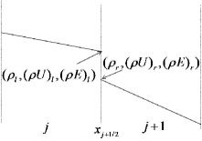
Figure 1: Reconstruction of the conservative variables at the cell interface.

By using the MUSCL-type limiter, a discontinuous reconstruction of the macroscopic flow variables can be obtained around the cell interface (see fig.1). The initial gas distribution function $f_{0}$ in (13) on both sides of a cell interface can be constructed as

$$\begin{array}[]{ll}f_{0}^{l}(\vec{x},\vec{u},\xi)=g_{0}^{l}(1+a^{l}(x-x_{j+1/2})+b^{l}(y-y_{i})-\tau(a^{l}u+b^{l}v+A^{l})),&x\leq x_{j+1/2},\\ \\ f_{0}^{r}(\vec{x},\vec{u},\xi)=g_{0}^{r}(1+a^{r}(x-x_{j+1/2})+b^{r}(y-y_{i})-\tau(a^{r}u+b^{r}v+A^{r})),&x>x_{j+1/2},\end{array}$$ (15)

where the Chapman-Enskog expansion up to the Navier-Stokes order has been used in the above initial reconstruction. Here $g_{0}^{l}$ and $g_{0}^{r}$ are the corresponding Maxwellians to $W^{l}=(\rho_{l},(\rho U)_{l},(\rho V)_{l},(\rho E)_{l})$ and $W^{r}=(\rho_{r},(\rho U)_{r},(\rho V)_{r},(\rho E)_{r})$ at both sides of the interface. The Maxwellian distribution function corresponding to $W=(\rho,(\rho U),(\rho V),(\rho E))$ has the form

$$g=\rho\left(\frac{\lambda}{\pi}\right)^{\frac{K+2}{2}}e^{\lambda((u-U)^{2}+(v-V)^{2}+\xi^{2})},$$ (16)

where $\lambda$ is equal to $m/2kT$, $m$ is the molecular mass, $k$ is the Boltzmann constant, and $T$ is the temperature. The equilibrium distribution functions around the cell interface can be modeled as

$$\begin{array}[]{ll}g^{l}(\vec{x},t,\vec{u},\xi)=g_{j+1/2}^{l}(1+\overline{a}^{l}(x-x_{j+1/2})+\overline{b}^{l}(y-y_{i})+\overline{A}^{l}t),&x\leq x_{j+1/2},\\ \\ g^{r}(\vec{x},t,\vec{u},\xi)=g_{j+1/2}^{r}(1+\overline{a}^{r}(x-x_{j+1/2})+\overline{b}^{r}(y-y_{i})+\overline{A}^{r}t),&x>x_{j+1/2}.\end{array}$$ (17)

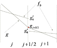
Figure 2: The modeling of the initial and equilibrium distribution functions at the cell interface for the BGK scheme without external forcing field.

In the case without external forcing term, $g_{j+1/2}^{l}$ and $g_{j+1/2}^{r}$ in the above equation are the same distribution functions, i.e., $g_{j+1/2}^{l}=g_{j+1/2}^{r}$ (see fig.2), which can be obtained using the conservation constraint (12) at $\vec{x}=\vec{x}_{j+1/2}$ and $t\rightarrow 0$,

$$\begin{array}[]{l}\quad\iiint g_{j+1/2}^{l}\psi\mathrm{d}u\mathrm{d}v\mathrm{d}\xi=\iiint g_{j+1/2}^{r}\psi\mathrm{d}u\mathrm{d}v\mathrm{d}\xi=W_{j+1/2}\\ \\ =\iiint_{u>0}f_{0}^{l}(\vec{x}_{j+1/2},\vec{u},\xi)\psi\mathrm{d}u\mathrm{d}v\mathrm{d}\xi+\iiint_{u<0}f_{0}^{r}(\vec{x}_{j+1/2},\vec{u},\xi)\psi\mathrm{d}u\mathrm{d}v\mathrm{d}\xi.\end{array}$$ (18)

Therefore, at the cell interface the final distribution function can be fully determined using the integral solution (13). The final distribution function can be written as

$$\begin{array}[]{l}\quad f(\vec{x}_{j+1/2},t,\vec{u},\xi)\\ \\ =\left\{\begin{array}[]{l}f^{l}(\vec{x}_{j+1/2},t,\vec{u},\xi)\quad\quad u\geq 0,\\ \\ f^{r}(\vec{x}_{j+1/2},t,\vec{u},\xi)\quad\quad u<0,\end{array}\right.\\ \\ =\left\{\begin{array}[]{l}\frac{1}{\tau}\int_{0}^{t}g^{l}(\vec{x}_{j+1/2}-\vec{u}(t-t^{\prime}),t^{\prime},\vec{u},\xi)e^{-(t-t^{\prime})/{\tau}}dt^{\prime}+e^{-t/{\tau}}{f_{0}^{l}}(\vec{x}_{j+1/2}-\vec{u}t),\quad\quad u\geq 0,\\ \\ \frac{1}{\tau}\int_{0}^{t}g^{r}(\vec{x}_{j+1/2}-\vec{u}(t-t^{\prime}),t^{\prime},\vec{u},\xi)e^{-(t-t^{\prime})/{\tau}}dt^{\prime}+e^{-t/{\tau}}{f_{0}^{r}}(\vec{x}_{j+1/2}-\vec{u}t),\quad\quad u<0,\end{array}\right.\end{array}$$ (19)

which can be used to evaluate the fluxes

$$\begin{array}[]{l}\quad F_{j+1/2}^{l}(t)=F_{j+1/2}^{r}(t)\\ \\ =\iiint_{u>0}uf^{l}(\vec{x}_{j+1/2},t,\vec{u},\xi)\psi\mathrm{d}u\mathrm{d}v\mathrm{d}\xi+\iiint_{u<0}uf^{r}(\vec{x}_{j+1/2},t,\vec{u},\xi)\psi\mathrm{d}u\mathrm{d}v\mathrm{d}\xi.\end{array}$$ (20)

The update of the cell averaged conservative variables becomes

$$W^{n+1}_{j}=W^{n}_{j}+\frac{1}{\Delta x}\int^{t_{n+1}}_{t_{n}}\left[F^{r}_{j-1/2}(t)-F^{l}_{j+1/2}(t)\right]dt+\frac{1}{\Delta y}\int^{t_{n+1}}_{t_{n}}\left[F^{r}_{i-1/2}(t)-F^{l}_{i+1/2}(t)\right]dt,$$ (21)

where $F^{l}_{j-1/2}(t)$ … $F^{r}_{i+1/2}(t)$ are the fluxes at the center of the cell interfaces.

The definitions and constructions of all parameters related to the spatial and temporal slopes, such as $a$, $b$ and $A$, can be found in [11] and [12].

In summary, at the cell interface $\vec{x}_{j+1/2}$ we can construct the equilibrium distribution functions $g_{j+1/2}^{l}$ and $g_{j+1/2}^{r}$ from initial distribution $f_{0}^{l}$ and $f_{0}^{r}$. Also, we can find fluxes $F_{j+1/2}^{l}(t)$ and $F_{j+1/2}^{r}(t)$ from the integral solution $f^{l}$ and $f^{r}$. Without external forcing field, all the particles running into the cell interface can freely cross it. Therefore, the equilibrium states and fluxes at the interface have unique values, i.e., $g_{j+1/2}^{l}=g_{j+1/2}^{r}$ and $F_{j+1/2}^{l}(t)=F_{j+1/2}^{r}(t)$. However, with the approximation of constant potential inside each cell and a potential jump at the cell interface, the modeling of equilibrium state $g$ around a cell interface has to be considered separately on different sides of the cell interface, where $g_{j+1/2}^{l}\neq g_{j+1/2}^{r}$ in general case. But, the mathematical formulae described in (17) and the integral solution in Eq.(19) can be still used. One of the main reason for the validity of the integral solution is that there is no gravitational force inside each cell. However, the construction of the equilibrium states and the calculation of fluxes will not be as simple as that in (18) and (20). In the evaluation of the equilibrium states and the fluxes, the physical principles for the particle transport discussed in the last section have to be used. In the next section, the determination of $g$ and fluxes will be described.

4 The symplecticity preserving BGK(SP-BGK) scheme

In this section, we will construct a well-balanced gas-kinetic scheme for hydrodynamic equations under gravitational field. In order to clarify the concepts, we are going to use a similar procedure as that of the construction of the BGK-NS scheme without external forcing field.

4.1 The initial data reconstruction

For a hydrostatic solution, the flow variables satisfy the conditions,

$$U=0,\,V=0,\,\lambda=constant,\,Ba=constant,$$ (22)

where $Ba=\rho e^{2\lambda\phi}$. In order to avoid introducing errors in the initial reconstruction for the hydrostatic case, it is reasonable to use the variables $(U,\,V,\,\lambda,\,Ba)$ in the reconstruction. More specifically, we firstly apply a MUSCL-type limiter to reconstruct the slopes of $(U,\,V,\,\lambda,\,Ba)$, i.e., $(S_{U},\,S_{V},\,S_{\lambda},\,S_{Ba})$ inside each cell. Since

$$\rho=\frac{Ba}{e^{2\lambda\phi}},\,\rho E=\frac{1}{2}\rho(U^{2}+V^{2})+\frac{K+2}{4\lambda}\rho,$$

we can get the corresponding slopes for other flow variables,

$$S_{\rho}=\frac{1}{e^{2\lambda\phi}}S_{Ba}-2\rho\phi S_{\lambda},S_{\rho U}=S_{\rho}U+\rho S_{U},S_{\rho V}=S_{\rho}V+\rho S_{V},$$

$$S_{\rho E}=\left[\frac{1}{2}(U^{2}+V^{2})+\frac{K+2}{4\lambda}\right]S_{\rho}+\rho\left[US_{U}+VS_{V}-\frac{K+2}{4\lambda^{2}}S_{\lambda}\right],$$

where $(S_{\rho},\,S_{\rho U},\,S_{\rho V},\,S_{\rho E})$ are the slopes of $(\rho,\,\rho U,\,\rho V,\,\rho E)$ inside that cell. Therefore, we can reconstruct $(\rho,\,\rho U,\,\rho V,\,\rho E)$ in each cell using their cell averaged quantities and the above slopes. Here, all slopes become zeros when the initial flow is in a hydrostatic state, and the reconstruction will not introduce numerical errors. In the general case, the above reconstruction works as well.

4.2 The gas-kinetic SP-BGK scheme

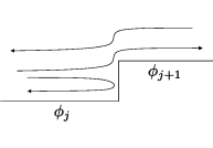
Figure 3: The particles’ movement at the interface with potential jump $\phi_{j}<\phi_{j+1}$.

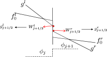
Figure 4: The modeling of the initial and equilibrium distribution functions at the cell interface for the SP-BGK scheme with a potential jump at the cell interface.

With the modeling of piecewise constant gravitational potential inside each cell, i.e., $\phi_{j}$ inside the $jth$ cell, there is a potential jump at the cell interface $\vec{x}_{j+1/2}$. It is obvious that the distribution function $f$ also satisfies the equation (10) inside each cell since there is no external forcing term inside each cell. Therefore, the similar framework used in the constructing BGK-NS scheme can be extended here to design the SP-BGK scheme with gravitational field. For example, with the initial reconstruction, the non-equilibrium states around each cell interface can be obtained. Also, due to the potential jump, the equilibrium states are different in the left and right hand sides of the interface, but the integral solution of the BGK model can be still used in the construction of the local solution separately around the cell interface. However, at the cell interface, we have to consider the effect of the potential jump on the particle movement. Since the equilibrium states, $g_{j+1/2}^{l}$ and $g_{j+1/2}^{r}$, and the fluxes, $F_{j+1/2}^{l}(t)$ and $F_{j+1/2}^{r}(t)$, involve the particle interaction with the potential jump, we will show that $g_{j+1/2}^{l}\neq g_{j+1/2}^{r}$ in Eq.(17)(see fig.4), and $F_{j+1/2}^{l}(t)\neq F_{j+1/2}^{r}(t)$ in the general case. Their determination depends on the particle transport modeling. The potential jump gives a critical speed $U_{c}=\sqrt{2|\phi_{j}-\phi_{j+1}|}$, which provides a threshold for the particle movement. Because of the potential jump, not all particles running into the cell interface could go through freely. Some may be reflected due to less kinetic energy to overcome the potential barrier (see fig.3). For these particles passing through the cell interface, their momentum and energy need to be modified due to particle acceleration during the transport process.

Without losing generality, we only discuss the case of $\phi_{j}<\phi_{j+1}$ in this subsection. Using similar methods and ideas, all the formulae for the case $\phi_{j}>\phi_{j+1}$ can be easily obtained. Let’s assume the initial reconstructed gas distribution at a cell interface before the interaction with the potential jump is

$$f(\vec{x}_{j+1/2},t,\vec{u},\xi)=\left\{\begin{array}[]{ll}f_{j}(\vec{x}_{j+1/2},t,\vec{u},\xi),&u\geq 0,\\ \\ f_{j+1}(\vec{x}_{j+1/2},t,\vec{u},\xi),&u<0.\end{array}\right.$$ (23)

Starting from the above distribution function, the particle collision with the potential jump changes distribution functions to $f_{j+1/2}^{l}(t,\vec{u},\xi)$ and $f_{j+1/2}^{r}(t,\vec{u},\xi)$ at the left and right hand sides of the cell interface respectively, which can be represented as

$$f_{j+1/2}^{l}(t,\vec{u},\xi)=\left\{\begin{array}[]{ll}f_{j}(\vec{x}_{j+1/2},t,\vec{u},\xi),&u>0,\\ \\ \tilde{f}_{j}(\vec{x}_{j+1/2},t,\vec{u},\xi),&0\geq u>-U_{c},\\ \\ \overline{f}_{j+1}(\vec{x}_{j+1/2},t,\vec{u},\xi),&u\leq-U_{c},\end{array}\right.$$ (24)

and

$$f_{j+1/2}^{r}(t,\vec{u},\xi)=\left\{\begin{array}[]{ll}\overline{f}_{j}(\vec{x}_{j+1/2},t,\vec{u},\xi),&u\geq 0,\\ \\ f_{j+1}(\vec{x}_{j+1/2},t,\vec{u},\xi),&u<0.\end{array}\right.$$ (25)

The definition of the above distribution functions is from the following physical consideration (see fig.3). Because the potential jump is only at the normal direction of the cell interface, it only affects the normal particle velocity, $u$. In (24), $\tilde{f}_{j}$ is the distribution function of the reflected particle in the $jth$ cell with the original distribution function $f_{j}$ which has a positive particle velocity less than $U_{c}$. Here $\overline{f}_{j+1}$ is the distribution function of the particle in the $jth$ cell coming from the $(j+1)th$ cell with the original distribution function $f_{j+1}$ with negative particle velocity. This particle has been accelerated in the negative normal direction after passing through the cell interface. Also, $\overline{f}_{j}$ is the distribution function of the particle in the $(j+1)th$ cell coming from the $jth$ cell with the original distribution function $f_{j}$ and positive velocity higher than $U_{c}$. This particle has been be decelerated in the positive normal direction after passing through the cell interface. Therefore, the effect of the potential jump modifies the distribution function, but the particle velocity moments of the modified distribution function and the original ones are related through the physical principles which have been introduced in section 2.

Here, we will show the procedure of the SP-BGK scheme first, then clarify the detailed derivation of the formulae for equilibrium states and fluxes.

Using particle free transport mechanism in Eq.(13) for the initial gas distribution function $f_{0}$, i.e., $f_{j}(\vec{x}_{j+1/2},t,\vec{u},\xi)=f_{0}^{l}(\vec{x}_{j+1/2}-\vec{u}t,\vec{u},\xi)$ and $f_{j+1}(\vec{x}_{j+1/2},t,\vec{u},\xi)=f_{0}^{r}(\vec{x}_{j+1/2}-\vec{u}t,\vec{u},\xi)$, and due to their interaction with the potential jump, the initial condition will be changed according to Eq.(24) and (25), from which two sets of conservative variables at different sides of the cell interface can be obtained,

$$\begin{array}[]{l}W_{j+1/2}^{l}=\iiint_{-\infty}^{\infty}f_{j+1/2}^{l}(t=0,\vec{u},\xi)\psi\mathrm{d}u\mathrm{d}v\xi\\ \\ \quad\quad\quad=\iiint_{0}^{+\infty}f_{j}(\vec{x}_{j+1/2},t=0,\vec{u},\xi)\psi\mathrm{d}u+\iiint_{-U_{c}}^{0}\tilde{f}_{j}(\vec{x}_{j+1/2},t=0,\vec{u},\xi)\psi\mathrm{d}u\mathrm{d}v\mathrm{d}\xi\\ \\ \qquad\quad\quad+\iiint_{-\infty}^{-U_{c}}\overline{f}_{j+1}(\vec{x}_{j+1/2},t=0,\vec{u},\xi)\psi\mathrm{d}u\mathrm{d}v\mathrm{d}\xi,\end{array}$$ (26)

and

$$\begin{array}[]{l}W_{j+1/2}^{r}=\iiint_{-\infty}^{\infty}f_{j+1/2}^{r}(t=0,\vec{u},\xi)\psi\mathrm{d}u\mathrm{d}v\xi\\ \\ \quad\quad\quad=\iiint_{0}^{+\infty}\overline{f}_{j}(\vec{x}_{j+1/2},t=0,\vec{u},\xi)\psi\mathrm{d}u\mathrm{d}v\mathrm{d}\xi+\iiint_{-\infty}^{0}f_{j+1}(\vec{x}_{j+1/2},t=0,\vec{u},\xi)\psi\mathrm{d}u\mathrm{d}v\mathrm{d}\xi,\end{array}$$ (27)

from which, two Maxwellians $g_{j+1/2}^{l}$ and $g_{j+1/2}^{r}$ in the equilibrium states (17) can be fully determined. Then, following the method used in the development of BGK-NS scheme [12], the final gas distribution at the left and right hand sides of a cell interface, i.e., $f^{l}$ and $f^{r}$ in (19), can be obtained. When choosing the integral solutions as the original distribution functions, i.e., $f_{j}(\vec{x}_{j+1/2},t,\vec{u},\xi)=f^{l}(\vec{x}_{j+1/2},t,\vec{u},\xi)$ and $f_{j+1}(\vec{x}_{j+1/2},t,\vec{u},\xi)=f^{r}(\vec{x}_{j+1/2},t,\vec{u},\xi)$, and considering their interactions with the potential jump, these distribution functions will be modified as Eq.(24) and (25), from which the corresponding fluxes at different sides of the cell interface can be determined,

$$\begin{array}[]{l}F_{j+1/2}^{l}(t)=\iiint_{-\infty}^{+\infty}uf_{j+1/2}^{l}(t,\vec{u},\xi)\psi\mathrm{d}u\mathrm{d}v\mathrm{d}\xi\\ \\ \qquad\qquad=\iiint_{0}^{+\infty}uf_{j}(\vec{x}_{j+1/2},t,\vec{u},\xi)\psi\mathrm{d}u+\int\int_{-U_{c}}^{0}u\tilde{f}_{j}(\vec{x}_{j+1/2},t,\vec{u},\xi)\psi\mathrm{d}u\mathrm{d}v\mathrm{d}\xi\\ \\ \qquad\qquad\quad+\iiint_{-\infty}^{-U_{c}}u\overline{f}_{j+1}(\vec{x}_{j+1/2},t,\vec{u},\xi)\psi\mathrm{d}u\mathrm{d}v\mathrm{d}\xi,\end{array}$$ (28)

and

$$\begin{array}[]{l}F_{j+1/2}^{r}(t)=\iiint_{-\infty}^{+\infty}uf_{j+1/2}^{r}(t,\vec{u},\xi)\psi\mathrm{d}u\mathrm{d}v\mathrm{d}\xi\\ \\ \qquad\qquad=\iiint_{0}^{+\infty}u\overline{f}_{j}(\vec{x}_{j+1/2},t,\vec{u},\xi)\psi\mathrm{d}u\mathrm{d}v\mathrm{d}\xi+\iiint_{-\infty}^{0}uf_{j+1}(\vec{x}_{j+1/2},t,\vec{u},\xi)\psi\mathrm{d}u\mathrm{d}v\mathrm{d}\xi.\end{array}$$ (29)

Note that due to the potential jump, in general we have $g_{j+1/2}^{l}\neq g_{j+1/2}^{r}$ and $F_{j+1/2}^{l}\neq F_{j+1/2}^{r}$. Finally, we can use (21) to update the cell averaged conservative variables.

In the above formulae (26), (27), (28) and (29), we need to find the $nth$ order velocity moments of the modified distribution functions, $\tilde{f}_{j}$, $\overline{f}_{j+1}$ and $\overline{f}_{j}$, which can be evaluated from the moments of the original distribution funcions $f_{j}$, $f_{j+1}$ and $f_{j}$ respectively by (9). Let’s figure out how to evaluate the $nth$ order normal velocity moments of $\tilde{f}_{j}(u)$, $\overline{f}_{j+1}(u)$ and $\overline{f}_{j}(u)$.

a. The $nth$-order normal velocity moments of $\tilde{f}_{j}$

Recall that $\tilde{f}_{j}$ is the distribution function of the reflected particle in the $jth$ cell. Assume that the normal particle velocity is $u$ before the reflection, and the distribution of the particle before reflection is $f_{j}(u)$ with $0<u<U_{c}$. After the reflection, its velocity becomes $u^{\prime}$ and $u^{\prime}=-u$, for these particles, (9) gives

$$\int_{-U_{c}}^{0}\tilde{f}_{j}(u^{\prime})(u^{\prime})^{n}\mathrm{d}u^{\prime}=\int_{U_{c}}^{0}f_{j}(u)u(-u)^{n-1}\mathrm{d}u=\int_{0}^{U_{c}}f_{j}(u)(-1)^{n}u^{n}\mathrm{d}u.$$ (30)

b. The $nth$-order normal velocity moments of $\overline{f}_{j+1}$

$\overline{f}_{j+1}$ is the distribution function of the particle in the $jth$ cell coming from the $(j+1)th$ cell. Its distribution function before crossing the potential jump is $f_{j+1}$ with normal velocity $u<0$. After passing through the interface, the normal velocity changes from $u$ to $u^{\prime}$, where $u$ and $u^{\prime}$ are related by the Hamiltonian preserving property, i.e.,

$$\frac{1}{2}u^{2}+\phi_{j+1}=\frac{1}{2}(u^{\prime})^{2}+\phi_{j}.$$

So, $u^{\prime}=-\sqrt{u^{2}+U_{c}^{2}}$, Eq.(9) gives

$$\int_{-\infty}^{-U_{c}}\overline{f}_{j+1}(u^{\prime})(u^{\prime})^{n}\mathrm{d}u^{\prime}=\int_{-\infty}^{0}f_{j+1}(u)(-1)^{n-1}u(u^{2}+U_{c}^{2})^{(n-1)/2}\mathrm{d}u.$$ (31)

c. The $nth$-order normal velocity moments of $\overline{f}_{j}$

$\overline{f}_{j}$ is the distribution function of the particle in the $(j+1)th$ cell coming from the $jth$ cell. Its distribution function before passing through the potential jump is $f_{j}$ with normal velocity $u>U_{c}$. After passing through the cell interface, the normal velocity changes to $u^{\prime}$. The relation between $u$ and $u^{\prime}$ becomes

$$\frac{1}{2}u^{2}+\phi_{j}=\frac{1}{2}(u^{\prime})^{2}+\phi_{j+1}.$$

So, $u^{\prime}=\sqrt{(u)^{2}-U_{c}^{2}}$, Eq.(9) deduces

$$\int_{0}^{+\infty}\overline{f}_{j}(u^{\prime})(u^{\prime})^{n}\mathrm{d}u=\int_{U_{c}}^{+\infty}f_{j}(u)u(u^{2}-U_{c}^{2})^{(n-1)/2}\mathrm{d}u.$$ (32)

Based on the above moment evaluations, we can get the formulae for $W_{j+1/2}^{l}$, $W_{j+1/2}^{r}$, $F_{j+1/2}^{l}(t)$ and $F_{j+1/2}^{r}(t)$ by (26)- (32) for the case $\phi_{j}<\phi_{j+1}$. The formulae for the case $\phi_{j}>\phi_{j+1}$ can be found similarly. All the formulae are given in the appendix for both 1-D and 2-D cases. Therefore, the SP-BGK scheme is presented.

4.3 Limiting Cases

a. The 1st order SP-BGK scheme

When all the slopes in the reconstruction are zeros, and all slopes $a$, $b$ and $A$ of the distribution function in (15) and (17) become zeros, the SP-BGK scheme becomes a 1st order scheme. Now, the distribution function in (13) becomes

$$f(\vec{x}_{j+1/2},t,\vec{u},\xi)=\left\{\begin{array}[]{ll}(1-e^{-t/\tau})g_{j+1/2}^{l}+e^{-t/\tau}g_{0}^{l},&u\geq 0,\\ \\ (1-e^{-t/\tau})g_{j+1/2}^{r}+e^{-t/\tau}g_{0}^{r},&u<0.\end{array}\right.$$

Or, with the definition of a small parameter $\varepsilon$, i.e., $0<\varepsilon<1$, the distribution function becomes

$$f(\vec{x}_{j+1/2},t,\vec{u},\xi)=\left\{\begin{array}[]{ll}(1-\varepsilon)g_{j+1/2}^{l}+\varepsilon g_{0}^{l},&u\geq 0,\\ \\ (1-\varepsilon)g_{j+1/2}^{r}+\varepsilon g_{0}^{r},&u<0,\end{array}\right.$$ (33)

which is called the 1st-order SP-BGK scheme.

b. The SP-KFVS scheme

When the collision time $\tau$ goes to $+\infty$, the distribution function in (19) becomes

$$\begin{array}[]{l}\quad f(\vec{x}_{j+1/2},t,\vec{u},\xi)=\left\{\begin{array}[]{l}f^{l}(\vec{x}_{j+1/2},t,\vec{u},\xi)\quad\quad u\geq 0,\\ \\ f^{r}(\vec{x}_{j+1/2},t,\vec{u},\xi)\quad\quad u<0,\end{array}\right.\\ \\ \qquad\qquad\qquad\qquad=\left\{\begin{array}[]{l}{f_{0}^{l}}(\vec{x}_{j+1/2}-\vec{u}t),\quad\quad u\geq 0,\\ \\ {f_{0}^{r}}(\vec{x}_{j+1/2}-\vec{u}t),\quad\quad u<0.\end{array}\right.\end{array}$$ (34)

The above solution solely comes from free transport and there is no contribution of the equilibrium states $g$ in the integral solution $f$. It equals to solve

$$f_{t}+\vec{u}\cdot\nabla f=0$$

directly when the initial distribution function is modeled as (15). In other words, we don’t consider particle collision here, and needn’t to model the equilibrium distribution function $g$ in (17). This is exactly the same scheme introduced in [14], which is called SP-KFVS scheme. It is actually a limiting case of the SP-BGK scheme.

In this section, with the assumption of piecewise constant gravitational potential, a SP-BGK scheme is presented. As will be presented in the next section, the SP-BGK scheme is a well-balanced scheme for the gravitational hydrodynamic system. This is the first well-balanced scheme, which has the shock capturing property as well in the general case.

5 Theoretical analysis

For simplicity, we are going to prove all the theorems in the 1-D case. But all the conclusions still hold for higher dimensions as well, because there is no dynamic difference in higher dimensions when the potential jump is modeled as a piecewise constant function.

In the current scheme, the updated flow variables inside each cell are the mass, momentum, and energy densities (kinetic + thermal ones). The gravitational energy is not explicitly included. However, for an isolated gravitational system, the total energy (kinetic + thermal + gravitational ones) conservation is a necessary condition in order to get a correct physical solution. In the following theorem, we are going first to prove that the conservation of total energy in the current kinetic scheme is satisfied.

Theorem 3.1: The SP-KFVS and SP-BGK schemes are mass and total energy conservative schemes.

Proof  The only difference between the SP-KFVS and SP-BGK schemes is that they have different original distribution functions $f_{j}(u)$ and $f_{j+1}(u)$. However, whatever $f_{j}(u)$ and $f_{j+1}(u)$ are, the mass and total energy are conserved when the fluxes are calculated by (92) and (93) or (94) and (95) in the appendix. The concept of conservation of a variable means that the change of that variable in any fixed domain depends only on the fluxes across the interfaces of that control volume. In the following proof, we assume the control volume consists of many cells between the cell index $K_{1}$ and $K_{2}$, where $K_{1}<K_{2}$. Then, we need to prove that the change of the mass and total energy in the control volume depends only on the fluxes at the interfaces $x_{K_{1}-1/2}$ and $x_{K_{2}+1/2}$. Without losing generality, we assume $\phi_{j}<\phi_{j+1}$ everywhere.

Mass conservation:

For mass, in each cell we have

$$\rho^{n+1}_{j}=\rho^{n}_{j}+\frac{1}{\Delta x}\int^{t_{n+1}}_{t_{n}}\left[F^{r}_{j-1/2,\rho}-F^{l}_{j+1/2,\rho}\right]\mathrm{d}t,$$ (35)

where $F^{r,l}_{j+1/2,\rho}$ are the mass fluxes. The total mass in the control volume is $\sum_{j=K_{1}}^{K_{2}}\rho_{j}$, and

$$\begin{array}[]{c}\sum_{j=K_{1}}^{K_{2}}\rho^{n+1}_{j}=\sum_{j=K_{1}}^{K_{2}}\rho^{n}_{j}+\frac{1}{\Delta x}\int^{t_{n+1}}_{t_{n}}\sum_{j=K_{1}}^{K_{2}}\left[F^{r}_{j-1/2,\rho}-F^{l}_{j+1/2,\rho}\right]\mathrm{d}t.\end{array}$$ (36)

From (92) and (93), we have

$$\begin{array}[]{l}\quad F^{l}_{j+1/2,\rho}\\ \\ =\int\int^{+\infty}_{0}f_{j}(u)u\mathrm{d}u\mathrm{d}\xi-\int\int^{U_{c}}_{0}f_{j}(u)u\mathrm{d}u\mathrm{d}\xi+\int\int^{0}_{-\infty}f_{j+1}(u)u\mathrm{d}u\mathrm{d}\xi\\ \\ =\int\int^{+\infty}_{U_{c}}f_{j}(u)u\mathrm{d}u\mathrm{d}\xi+\int\int^{0}_{-\infty}f_{j+1}(u)u\mathrm{d}u\mathrm{d}\xi\\ \\ =F^{r}_{j+1/2,\rho}.\end{array}$$ (37)

Therefore, from (36) and (37),

$$\begin{array}[]{c}\sum_{j=K_{1}}^{K_{2}}\rho^{n+1}_{j}=\sum_{j=K_{1}}^{K_{2}}\rho^{n}_{j}+\frac{1}{\Delta x}\int^{t_{n+1}}_{t_{n}}\left[F^{r}_{K_{1}-1/2,\rho}-F^{l}_{K_{2}+1/2,\rho}\right]\mathrm{d}t,\end{array}$$ (38)

which gives the mass conservation in the computational domain.

Total energy conservation:

The kinetic energy and thermal energy, i.e., $\rho E$, is updated by

$$(\rho E)^{n+1}_{j}=(\rho E)^{n}_{j}+\frac{1}{\Delta x}\int^{t_{n+1}}_{t_{n}}\left[F^{r}_{j-1/2,\rho E}-F^{l}_{j+1/2,\rho E}\right]\mathrm{d}t,$$ (39)

where $F^{r,l}_{j+1/2,\rho E}$ are the fluxes of $\rho E$. Because the external potential $\phi$ is independent of time, the potential energy, i.e., $\rho\phi$ is updated by

$$\rho^{n+1}_{j}\phi_{j}=\rho^{n}_{j}\phi_{j}+\frac{1}{\Delta x}\int^{t_{n+1}}_{t_{n}}\left[F^{r}_{j-1/2,\rho}\phi_{j}-F^{l}_{j+1/2,\rho}\phi_{j}\right]\mathrm{d}t.$$ (40)

With the definition of total energy $TE=\rho E+\rho\phi$, we get

$$\begin{array}[]{l}TE^{n+1}_{j}=TE^{n}_{j}+\frac{1}{\Delta x}\int^{t_{n+1}}_{t_{n}}\left[F^{r}_{j-1/2,\rho}\phi_{j}-F^{l}_{j+1/2,\rho}\phi_{j}\right.\\ \\ \qquad\qquad\left.+F^{r}_{j-1/2,\rho E}-F^{l}_{j+1/2,\rho E}\right]\mathrm{d}t.\end{array}$$ (41)

The updating of the total energy in the control volume (i.e. $\sum_{j=K_{1}}^{K_{2}}TE_{j}$) becomes

$$\begin{array}[]{l}\sum_{j=K_{1}}^{K_{2}}TE^{n+1}_{j}=\sum_{j=K_{1}}^{K_{2}}TE^{n}_{j}+\frac{1}{\Delta x}\int^{t_{n+1}}_{t_{n}}\sum_{j=K_{1}}^{K_{2}}\left[F^{r}_{j-1/2,\rho}\phi_{j}\right.\\ \\ \qquad\qquad\qquad\quad\left.-F^{l}_{j+1/2,\rho}\phi_{j}+F^{r}_{j-1/2,\rho E}-F^{l}_{j+1/2,\rho E}\right]\mathrm{d}t.\end{array}$$ (42)

According to (92) and (93), we get

$$\begin{array}[]{l}F^{l}_{j+1/2,\rho E}=\int\int^{+\infty}_{0}f_{j}(u)\frac{1}{2}(u^{3}+u\xi)\mathrm{d}u\mathrm{d}\xi+\int\int^{U_{c}}_{0}f_{j}(u)\frac{1}{2}(-u^{3}-u\xi)\mathrm{d}u\mathrm{d}\xi\\ \\ \qquad\qquad\quad+\int\int^{0}_{-\infty}f_{j+1}(u)\frac{1}{2}(u(u^{2}+U_{c}^{2})+u\xi)\mathrm{d}u\mathrm{d}\xi,\\ \\ F^{r}_{j+1/2,\rho E}=\int\int^{+\infty}_{U_{c}}f_{j}(u)\frac{1}{2}(u(u^{2}-U_{c}^{2})+u\xi)\mathrm{d}u\mathrm{d}\xi\\ \\ \qquad\qquad\quad+\int\int^{0}_{-\infty}f_{j+1}(u)\frac{1}{2}(u^{3}+u\xi)\mathrm{d}u\mathrm{d}\xi.\end{array}$$ (43)

A direct calculation gives

$$F^{r}_{j+1/2,\rho E}-F^{l}_{j+1/2,\rho E}=F^{l}_{j+1/2,\rho}(\phi_{j+1}-\phi_{j})=F^{r}_{j+1/2,\rho}(\phi_{j+1}-\phi_{j}).$$ (44)

So, from (42) and (44), the total energy update becomes

$$\begin{array}[]{l}\sum_{j=K_{1}}^{K_{2}}TE^{n+1}_{j}=\sum_{j=K_{1}}^{K_{2}}TE^{n}_{j}+\frac{1}{\Delta x}\int^{t_{n+1}}_{t_{n}}\left[F^{r}_{K_{1}-1/2,\rho}\phi_{K_{1}}\right.\\ \\ \qquad\qquad\qquad\quad\left.-F^{l}_{K_{2}+1/2,\rho}\phi_{K_{2}}+F^{r}_{K_{1}-1/2,\rho E}-F^{l}_{K_{2}+1/2,\rho E}\right]\mathrm{d}t,\end{array}$$ (45)

which guarantees the total energy conservation in the whole computational domain. Based on the above proof, the SP-BGK and SP-KFVS schemes are conservative methods. Therefore, the above two schemes can give the correct shock location even with the external gravitational forcing terms. This is a generalization of Lax-Wendroff theorem to the system with gravitational source term [5].

Lemma 3.2: The density $\rho(x)$ in a hydrostatic state under the gravitational field $\phi(x)$ satisfies

$$\rho(x)=C_{1}e^{-2\tilde{\lambda}\phi(x)},$$ (46)

where $C_{1}$ and $\tilde{\lambda}$ are constants.

Proof  For a hydrostatic solution under the gravitational field $\phi(x)$, we have

$$p_{x}=-\rho\phi_{x},T={\mbox{constant}},U=0.$$ (47)

Since $T={\mbox{constant}}$ and $\lambda=m/2kT$, we know $\lambda=\tilde{\lambda}$, where $\tilde{\lambda}$ is also a constant. Then from (47) and the ideal gas equation of state

$$p=\frac{1}{2\tilde{\lambda}}\rho,$$

we have

$$\frac{1}{2\tilde{\lambda}}\rho_{x}=-\rho\phi_{x}.$$

Therefore, with a constant, $C_{1}$, the solution becomes

$$\rho(x)=C_{1}e^{-2\tilde{\lambda}\phi(x)}.$$

Remark: without losing generality, in the following proofs, we let $C_{1}=1$ for the hydrostatic solution. So, in the hydrostatic case, the state has the form

$$\rho=e^{-2\tilde{\lambda}\phi(x)},\,U=0,$$ (48)

where $\tilde{\lambda}$ is a constant. Numerically, if we let the potential $\phi(x)$ be a constant, $\phi_{j}$, in the $jth$ cell, then

$$\rho_{j+1}=\rho_{j}e^{-2\tilde{\lambda}(\phi_{j+1}-\phi_{j})},\,U_{j}=0,$$ (49)

where $\rho_{j}$ and $U_{j}$ are cell average quantities in that cell.

Lemma 3.3: For the two equilibrium states $W^{l}_{j+1/2}=(\rho^{l}_{j+1/2},\,(\rho U)^{l}_{j+1/2},\,(\rho E)^{l}_{j+1/2})$ and $W^{r}_{j+1/2}=(\rho^{r}_{j+1/2},\,(\rho U)^{r}_{j+1/2},\,(\rho E)^{r}_{j+1/2})$, they have the following properties when the initial flow is in a hydrostatic state.

1. Both velocities are equal to zero, i.e.,

$$U^{l}_{j+1/2}=U^{r}_{j+1/2}=0.$$ (50)

2. They have the same temperature at both sides of all cell interfaces, i.e.

$$\lambda^{l}_{j+1/2}=\lambda^{r}_{j+1/2}=\tilde{\lambda},$$ (51)

where $\lambda$ satisfies

$$\rho E-\frac{1}{2}\rho U^{2}=\rho\frac{K+1}{4\lambda},$$ (52)

macroscopically with $K=(3-\gamma)/(\gamma-1)$ in 1-D, and $\tilde{\lambda}$ has the constant value $\lambda$ of the hydrostatic solution.

3. The densities at the same cell interface satisfy

$$\rho^{r}_{j+1/2}=\rho^{l}_{j+1/2}e^{-2\tilde{\lambda}(\phi_{j+1}-\phi_{j})}$$ (53)

4. In the same cell,

$$\rho^{l}_{j+1/2}=\rho^{r}_{j-1/2}$$ (54)

Proof  As the definition, $W^{l}_{j+1/2}$ and $W^{r}_{j+1/2}$ are determined by (88) and (89) or (90) and (91) for $\phi_{j}<\phi_{j+1}$ or $\phi_{j}>\phi_{j+1}$ when $f_{j}(u)=g_{j}(u)$, where $g_{j}(u)$ is a Maxwellian corresponding to the cell average conservative variables, $(\rho_{j},\,(\rho U)_{j},\,(\rho E)_{j})$. Here, we only prove the case for $\phi_{j}<\phi_{j+1}$. The other case can be proved similarly. From direct calculation, we can get

$$\rho^{l}_{j+1/2}=\frac{\rho_{j}}{2}+\rho_{j}(\frac{\tilde{\lambda}}{\pi})^{\frac{1}{2}}\int_{-U_{c}}^{0}e^{-\tilde{\lambda}u^{2}}\mathrm{d}u-\rho_{j+1}(\frac{\tilde{\lambda}}{\pi})^{\frac{1}{2}}U_{c}+\rho_{j+1}\tilde{\lambda}(\frac{\tilde{\lambda}}{\pi})^{\frac{1}{2}}\int_{0}^{+\infty}e^{-\tilde{\lambda}t}\sqrt{t+U_{c}^{2}}\mathrm{d}t,$$ (55)

$$\rho^{r}_{j+1/2}=\rho_{j}\tilde{\lambda}(\frac{\tilde{\lambda}}{\pi})^{\frac{1}{2}}\int_{U_{c}^{2}}^{+\infty}e^{-\tilde{\lambda}t}\sqrt{t-U_{c}^{2}}\mathrm{d}t+\frac{\rho_{j+1}}{2},$$ (56)

$$(\rho U)^{l}_{j+1/2}=(\rho U)^{r}_{j+1/2}=0,$$ (57)

$$\begin{array}[]{l}(\rho E)^{l}_{j+1/2}=\frac{K}{4\tilde{\lambda}}\rho^{l}_{j+1/2}+\frac{\rho_{j}}{8\tilde{\lambda}}-\frac{\rho_{j}}{4\tilde{\lambda}}\sqrt{\frac{\tilde{\lambda}}{\pi}}e^{-\tilde{\lambda}U_{c}^{2}}U_{c}+\frac{\rho_{j}}{4\tilde{\lambda}}\sqrt{\frac{\tilde{\lambda}}{\pi}}\int_{-U_{c}}^{0}e^{-\tilde{\lambda}u^{2}}\mathrm{d}u\\ \\ \qquad\qquad\qquad+\frac{\rho_{j+1}}{4}\sqrt{\frac{\tilde{\lambda}}{\pi}}\int_{0}^{+\infty}e^{-\tilde{\lambda}t}\sqrt{t+U_{c}^{2}}\mathrm{d}t,\end{array}$$ (58)

and

$$(\rho E)^{r}_{j+1/2}=\frac{K}{4\tilde{\lambda}}\rho^{r}_{j+1/2}+\frac{\rho_{j}}{4}\sqrt{\frac{\tilde{\lambda}}{\pi}}\int_{U_{c}^{2}}^{+\infty}e^{-\tilde{\lambda}t}\sqrt{t-U_{c}^{2}}\mathrm{d}t+\frac{\rho_{j+1}}{8\tilde{\lambda}},$$ (59)

where $U_{c}=\sqrt{2(\phi_{j+1}-\phi_{j})}$.

1. From (55) and (56), we can easily see that $\rho^{l}_{j+1/2}>0$ and $\rho^{r}_{j+1/2}>0$ when $\rho_{j}>0$ and $\rho_{j+1}>0$. Since $U=\rho U/\rho$, from (57), we know that

$$U^{l}_{j+1/2}=U^{r}_{j+1/2}=0.$$

2. From (55),

$$\begin{array}[]{l}\rho^{l}_{j+1/2}\,\frac{K+1}{4\lambda^{l}_{j+1/2}}=\frac{K}{4\lambda^{l}_{j+1/2}}\rho^{l}_{j+1/2}+\frac{\rho_{j}}{8\lambda^{l}_{j+1/2}}+\frac{\rho_{j+1}}{4\lambda^{l}_{j+1/2}}\sqrt{\frac{\tilde{\lambda}}{\pi}}U_{c}+\frac{\rho_{j}}{4\lambda^{l}_{j+1/2}}\sqrt{\frac{\tilde{\lambda}}{\pi}}\int_{-U_{c}}^{0}e^{-\tilde{\lambda}u^{2}}\mathrm{d}u\\ \\ \qquad\qquad\qquad\quad+\frac{\rho_{j+1}}{4\lambda^{l}_{j+1/2}}\tilde{\lambda}\sqrt{\frac{\tilde{\lambda}}{\pi}}\int_{0}^{+\infty}e^{-\tilde{\lambda}t}\sqrt{t+U_{c}^{2}}\mathrm{d}t.\end{array}$$ (60)

Since $(\rho E)^{l}_{j+1/2}-\frac{1}{2}\rho^{l}_{j+1/2}(U^{l}_{j+1/2})^{2}=\rho^{l}_{j+1/2}\,\frac{K+1}{4\lambda^{l}_{j+1/2}}$ and $U^{l}_{j+1/2}=0$, we have

$$(\rho E)^{l}_{j+1/2}-\rho^{l}_{j+1/2}\frac{K+1}{4\lambda^{l}_{j+1/2}}=0.$$ (61)

Therefore, substitute (49), (58) and (60) into (61), we get

$$\begin{array}[]{l}(\lambda^{l}_{j+1/2}-\tilde{\lambda})\left\{\frac{1}{\lambda^{l}_{j+1/2}\tilde{\lambda}}(\frac{K}{4}\rho^{l}_{j+1/2}+\frac{\rho_{j}}{8}-\frac{\rho_{j}}{4}\sqrt{\frac{\tilde{\lambda}}{\pi}}e^{-\tilde{\lambda}U_{c}^{2}}U_{c}\right.\\ \\ \left.+\frac{\rho_{j}}{4}\sqrt{\frac{\tilde{\lambda}}{\pi}}\int_{-U_{c}}^{0}e^{-\tilde{\lambda}u^{2}}\mathrm{d}u)+\frac{1}{\lambda^{l}_{j+1/2}}\frac{\rho_{j+1}}{4}\sqrt{\frac{\tilde{\lambda}}{\pi}}\int_{0}^{+\infty}e^{-\tilde{\lambda}t}\sqrt{t+U_{c}^{2}}\mathrm{d}t\right\}=0.\end{array}$$ (62)

Because $e^{-\tilde{\lambda}u^{2}}$ is a monotonic increasing function on $[-U_{c},0]$, so

$$\frac{\rho_{j}}{4}\sqrt{\frac{\lambda}{\pi}}\int_{-U_{c}}^{0}e^{-\lambda u^{2}}\mathrm{d}u-\frac{\rho_{j}}{4}\sqrt{\frac{\lambda}{\pi}}e^{-\lambda U_{c}^{2}}U_{c}>0.$$ (63)

Then we know the summation in the brace $\{...\}$ of (62) is strictly larger than zero. Therefore,

$$\lambda^{l}_{j+1/2}=\tilde{\lambda}.$$

has to be satisfied.

Similarly, we can have

$$(\lambda^{r}_{j+1/2}-\tilde{\lambda})\{\frac{1}{\lambda^{r}_{j+1/2}\tilde{\lambda}}(\frac{K}{4}\rho^{r}_{j+1/2}+\frac{\rho_{j+1}}{8})+\frac{1}{\lambda^{r}_{j+1/2}}\frac{\rho_{j}}{4}\sqrt{\frac{\tilde{\lambda}}{\pi}}\int_{U_{c}^{2}}^{+\infty}e^{-\tilde{\lambda}t}\sqrt{t-U_{c}^{2}}\mathrm{d}t\}=0.$$

Again, the summation in the brace $\{...\}$ is strictly larger than zero. So,

$$\lambda^{r}_{j+1/2}=\tilde{\lambda}.$$

3. It is easy to prove that

$$\int_{-U_{c}}^{0}e^{-\tilde{\lambda}u^{2}}\mathrm{d}u=e^{-\lambda U_{c}^{2}}U_{c}+2\tilde{\lambda}\int_{-U_{c}}^{0}e^{-\tilde{\lambda}u^{2}}u^{2}\mathrm{d}u,$$ (64)

and

$$2\int_{-U_{c}}^{0}e^{-\tilde{\lambda}u^{2}}u^{2}\mathrm{d}u=\int_{0}^{U_{c}^{2}}e^{-\tilde{\lambda}x}\sqrt{x}\mathrm{d}x.$$ (65)

So,   $\rho^{r}_{j+1/2}=\rho^{l}_{j+1/2}e^{-2\tilde{\lambda}(\phi_{j+1}-\phi_{j})},$

$\xLongleftrightarrow{(\ref{eq:equi-densl}),(\ref{eq:equi-densr})}$ $\tilde{\lambda}\int_{U_{c}^{2}}^{+\infty}e^{-\tilde{\lambda}t}\sqrt{t-U_{c}^{2}}\mathrm{d}t=\int_{-U_{c}}^{0}e^{-\tilde{\lambda}(u^{2}+U_{c}^{2})}\mathrm{d}u-U_{c}e^{-2\tilde{\lambda}U_{c}^{2}}+\tilde{\lambda}e^{-2\tilde{\lambda}U_{c}^{2}}\int_{0}^{+\infty}e^{-\tilde{\lambda}t}\sqrt{t+U_{c}^{2}}\mathrm{d}t,$ $\xLongleftrightarrow{(\ref{eq:lem2-5})}$ $\int_{U_{c}^{2}}^{+\infty}e^{-\tilde{\lambda}t}\sqrt{t-U_{c}^{2}}\mathrm{d}t=2e^{-\tilde{\lambda}U_{c}^{2}}\int_{-U_{c}}^{0}e^{-\tilde{\lambda}u^{2}}u^{2}\mathrm{d}u+e^{-2\tilde{\lambda}U_{c}^{2}}\int_{0}^{+\infty}e^{-\tilde{\lambda}t}\sqrt{t+U_{c}^{2}}\mathrm{d}t,$

$\xLongleftrightarrow{left:x=t-U_{c}^{2};right:x=t+U_{c}^{2}}$ $\int_{0}^{+\infty}e^{-\tilde{\lambda}x}\sqrt{x}\mathrm{d}x=2\int_{-U_{c}}^{0}e^{-\tilde{\lambda}u^{2}}u^{2}\mathrm{d}u+\int_{U_{c}^{2}}^{+\infty}e^{-\tilde{\lambda}x}\sqrt{x}\mathrm{d}x$

$\Longleftrightarrow\int_{0}^{U_{c}^{2}}e^{-\tilde{\lambda}x}\sqrt{x}\mathrm{d}x=2\int_{-u_{c}}^{0}e^{-\tilde{\lambda}u^{2}}u^{2}\mathrm{d}u.$

Therefore, from (65), we can conclude that

$$\rho^{r}_{j+1/2}=\rho^{l}_{j+1/2}e^{-2\tilde{\lambda}(\phi_{j+1}-\phi_{j})}.$$

4.   $\rho^{l}_{j+1/2}=\rho^{r}_{j-1/2},$

$\xLongleftrightarrow{(\ref{eq:equi-densl}),(\ref{eq:equi-densr})}$  $\frac{\rho_{j}}{2}+\rho_{j}(\frac{\tilde{\lambda}}{\pi})^{\frac{1}{2}}\int_{-U_{c}}^{0}e^{-\tilde{\lambda}u^{2}}\mathrm{d}u-\rho_{j+1}(\frac{\tilde{\lambda}}{\pi})^{\frac{1}{2}}U_{c}+\rho_{j+1}\tilde{\lambda}(\frac{\tilde{\lambda}}{\pi})^{\frac{1}{2}}\int_{0}^{+\infty}e^{-\tilde{\lambda}t}\sqrt{t+U_{c}^{2}}\mathrm{d}t$

$=\rho_{j-1}\tilde{\lambda}(\frac{\tilde{\lambda}}{\pi})^{\frac{1}{2}}\int_{U_{c}^{2}}^{+\infty}e^{-\tilde{\lambda}t}\sqrt{t-U_{c}^{2}}\mathrm{d}t+\frac{\rho_{j}}{2},$

$\xLongleftrightarrow{(\ref{eq:hydro-soln-numer})}\rho_{j}\int_{-U_{c}}^{0}e^{-\tilde{\lambda}u^{2}}\mathrm{d}u-\rho_{j}e^{-\tilde{\lambda}U_{c}^{2}}U_{c}+\rho_{j}\tilde{\lambda}\int_{U_{c}^{2}}^{+\infty}e^{-\tilde{\lambda}x}\sqrt{x}\mathrm{d}x=\rho_{j}\tilde{\lambda}\int_{0}^{+\infty}e^{-\tilde{\lambda}x}\sqrt{x}\mathrm{d}x,$

$\xLongleftrightarrow{(\ref{eq:lem2-5})}$ $2\tilde{\lambda}\rho_{j}\int_{-U_{c}}^{0}e^{-\tilde{\lambda}u^{2}}u^{2}\mathrm{d}u+\rho_{j}\tilde{\lambda}\int_{U_{c}^{2}}^{+\infty}e^{-\tilde{\lambda}x}\sqrt{x}\mathrm{d}x=\rho_{j}\tilde{\lambda}\int_{0}^{+\infty}e^{-\tilde{\lambda}x}\sqrt{x}\mathrm{d}x.$

From (65), we know that the last equality holds. Therefore,

$$\rho^{l}_{j+1/2}=\rho^{r}_{j-1/2}.$$

Remark: the above lemma, especially part 2, illustrates that starting from a hydrostatic state with the same temperature, the constructed equilibrium states at both sides of a cell interface have the equal temperature as well. In order words, in the hydrostatic case, the particle interaction with the potential barrier and the particle collisions among themselves never alter the equilibrium temperature both sides of a cell interface. This is consistent with the second law of thermodynamics. Otherwise, the temperature differences generated by the particle collisions could be used drive an engine and a pure work could have been extracted from an initially isothermal system. This violates the 2nd-law of thermodynamics.

Theorem 3.4: For a well-balanced kinetic scheme, the equilibrium distribution function must be an ”Exact Maxwellian”.

Proof  In order to keep the hydrostatic solution (49) the numerical mass flux at both sides of a cell interface must be zero.

Without losing generality, we only consider the case for $\phi_{j+1}>\phi_{j}$. Since the gas must be isotropic, we can assume the equilibrium distribution function is $\rho(x)G(u^{2})$ and define $a=\sqrt{2(\phi_{j+1}-\phi_{j})}$, then we require

$$F^{r}_{j+1/2,\rho}=\int^{+\infty}_{a}\rho_{j}G(u^{2})u\mathrm{d}u+\int^{0}_{-\infty}\rho_{j+1}G(u^{2})u\mathrm{d}u=0,$$ (66)

where $F^{r}_{j+1/2,\rho}$ is the mass flux at the right side of the interface. Because of (49), we have

$$\frac{1}{2}\int^{+\infty}_{a^{2}}G(x)\mathrm{d}x+e^{-\lambda a^{2}}\int^{0}_{-\infty}G(u^{2})u\mathrm{d}u=0.$$ (67)

Take the derivative of (67) with $a^{2}$, we get

$$-\frac{1}{2}G(a^{2})-\lambda e^{-\lambda a^{2}}\int^{0}_{-\infty}G(u^{2})u\mathrm{d}u=0.$$ (68)

It is obvious from (68) that

$$G(a^{2})\sim e^{-\lambda a^{2}},$$ (69)

which means that the equilibrium distribution function is an exact Maxewellian distribution.

Theorem 3.5: Both the 1st-order SP-KFVS and SP-BGK schemes are well-balanced schemes.

Proof  In order to prove a scheme to be a well-balanced one, we only need to verify that the scheme can keep the hydrostatic solution (48) forever. Numerically, the initial condition for this case is given by (49) in the $jth$ cell. At the next time step, the above solution must be kept by the well-balanced numerical scheme, i.e., $W^{n+1}_{j}=W^{n}_{j}$. From (21), we must have

$$F^{r}_{j-1/2}=F^{l}_{j+1/2}.$$ (70)

Therefore, to complete the proof, we have to show that mass fluxes ($F^{r,l}_{j+1/2,\rho}$), momentum fluxes ($F^{r,l}_{j+1/2,\rho U}$) and energy fluxes ($F^{r,l}_{j+1/2,\rho E}$) satisfy the condition (70) respectively.

The $1st$-order SP-KFVS scheme: the original distribution function at the cell interface is

$$f(x_{j+1/2},t,u,\xi)=\left\{\begin{array}[]{ll}g_{j}(u),&u\geq 0,\\ \\ g_{j+1}(u),&u<0,\end{array}\right.$$ (71)

where $g_{j}(u)$ is the Maxwellian corresponding to $(\rho_{j},\,(\rho U)_{j},\,(\rho E)_{j})$. The proof is only a direct calculation of the fluxes at the interface using (92) and (93) or (94) and (95) in two different cases for $\phi_{j}<\phi_{j+1}$ or $\phi_{j}>\phi_{j+1}$. Also the initial hydrostatic condition (49) will be used. The results are the followings.
a. For mass flux,

$$F^{l}_{j+1/2,\rho}=F^{r}_{j+1/2,\rho}=0.$$ (72)

b. For momentum flux,

$$F^{l}_{j+1/2,\rho U}=F^{r}_{j-1/2,\rho U}=\frac{\rho_{j}}{2\lambda}.$$ (73)

c. For energy flux,

$$F^{l}_{j+1/2,\rho E}=F^{r}_{j+1/2,\rho E}=0.$$ (74)

Hence, the first order $1st$ order SP-KFVS scheme is a well-balanced one.

The 1st order SP-BGK scheme: the original distribution function is

$$f(x_{j+1/2},t,u,\xi)=\left\{\begin{array}[]{ll}(1-\epsilon)g_{j}(u)+\epsilon g_{j+1/2}^{l}(u),&u\geq 0,\\ \\ (1-\epsilon)g_{j+1}(u)+\epsilon g_{j+1/2}^{r}(u),&u<0,\end{array}\right.$$ (75)

where $\epsilon$ is a constant between $0$ and $1$, $g_{j}(u)$ is the same as in the proof for the 1st order SP-KFVS scheme, $g_{j+1/2}^{l}$ and $g_{j+1/2}^{r}$ are two equilibrium states corresponding to $W_{j+1/2}^{l}$ and $W_{j+1/2}^{r}$ respectively. Here, $W_{j+1/2}^{l}$ and $W_{j+1/2}^{r}$ are the macroscopic variables calculated by (88) and (89) or (90) and (91) when

$$f_{j}(u)=g_{j}(u)\,\,\textrm{and}\,\,f_{j+1}(u)=g_{j+1}(u).$$

So, the fluxes are the linear combination of two kinds of fluxes $F_{1}$ and $F_{2}$ calculated by

$$f_{1}=\left\{\begin{array}[]{ll}g_{j}(u),&u\geq 0,\\ \\ g_{j+1}(u),&u<0,\end{array}\right.\,\,\textrm{and}\,\,f_{2}=\left\{\begin{array}[]{ll}g_{j+1/2}^{l}(u),&u\geq 0,\\ \\ g_{j+1/2}^{r}(u),&u<0,\end{array}\right.$$

respectively.

From the above proof for the 1st order SP-KFVS scheme, we know that the first kind fluxes $F_{1}$ can satisfy (70) itself. Therefore, we only need to prove that $F_{2}$ can satisfy (70), too. Note that in the proof for the 1st order SP-KFVS scheme, the hydrostatic initial condition is the key. But from the Lemma 3.3, we can see that the equilibrium states also satisfy the hydrostatic initial condition. So, similarly, we get the following results for the fluxes corresponding to $f_{2}$ from a direct calculation by using (92) and (93) or (94) and (95) in two different cases for $\phi_{j}<\phi_{j+1}$ or $\phi_{j}>\phi_{j+1}$.
a. For mass flux,

$$F^{l}_{j+1/2,\rho}=F^{r}_{j+1/2,\rho}=0.$$ (76)

b. For momentum flux,

$$\begin{array}[]{l}F^{l}_{j+1/2,\rho U}=\frac{\rho^{l}_{j+1/2}}{2\lambda^{l}_{j+1/2}},\\ \\ F^{r}_{j-1/2,\rho U}=\frac{\rho^{r}_{j-1/2}}{2\lambda^{r}_{j-1/2}}.\end{array}$$ (77)

Based on Eq.(51) and (54),

$$F^{l}_{j+1/2,\rho U}=F^{r}_{j-1/2,\rho U}.$$ (78)

c. For energy flux,

$$F^{l}_{j+1/2,\rho E}=F^{r}_{j+1/2,\rho E}=0.$$ (79)

From all the above proofs, we can conclude that both the 1st-order SP-KFVS and SP-BGK schemes can keep the initial hydrostatic solution forever. Therefore, they are well-balanced schemes.

Remark: The 2nd order SP-KFVS and SP-BGK schemes are well-balanced schemes.

We use $(U,\lambda,\rho e^{2\lambda\phi})$ to do the reconstruction. All the three variables are constants when the solution is in a hydrostatic state. So, the slopes are all zeros after using the MUSCL-type limiter. In other words, the 2nd-order schemes go back to the 1st-order method when the solution is in hydrostatic state, which can be kept forever. Therefore, the 2nd-order schemes are also well-balanced schemes.

6 Numerical examples

In this section, we will present numerical results of four 1-D examples by using $1^{st}$ and $2^{nd}$ order SP-KFVS and SP-BGK schemes, and also a 2-D example using a $2^{nd}$-order SP-BGK scheme. Each of the examples is very sensitive to the accuracy of the scheme. Some of the tests run for millions of numerical steps. If the scheme is not a well-balanced one, the accumulation of any small numerical error would become significant for such a long time integration [10].

6.1 Shock tube under gravitational field

This case is the standard Sod test under gravitational field. The computational domain is $x\in[0,1]$ which is divided into $100$ cells. Reflection boundary condition is used on both ends. The initial condition is

$$\rho=1.0,U=0.0,p=1.0\textrm{ for }x\leq 0.5,$$

and

$$\rho=0.125,U=0.0,p=0.1\textrm{ for }x>0.5.$$

The gravitational force $G$ takes a value $G=-1.0$ in the x-direction. So the potential jump at each cell interface becomes

$$\Delta\phi=-G\Delta x=0.01.$$

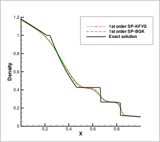
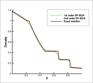
Figure 5: Density distributions for the shock tube problem under gravitational field.

The computational results at $t=0.2$ are presented in fig. 5,  6 for the density, pressure and velocity from the $1^{st}$-order SP-KFVS, $1^{st}$ and $2^{nd}$-order SP-BGK schemes. From these figures, we can find that SP-KFVS scheme has larger numerical dissipation than that in SP-BGK scheme, and $1^{st}$-order scheme is more dissipative than $2^{nd}$-order one. The results calculated by the $2^{nd}$ order SP-BGK scheme fits the exact solution very well. Due to the gravitational force, the density distribution inside the tube is pulled back in the negative x-direction. In some region, the flow velocity even becomes negative.

6.2 Isolated gravitational system with adiabatic wall

The second test case is also on a computational domain $x\in[0,1]$ with $50$ cells. There are limited number of gravitational potential jumps at locations $x=0.21,0.41,0.61$ and $0.81$ with a large value

$$\Delta\Phi=2.0.$$

The initial flow distributions inside the domain has constant values of

$$\rho=1.0,\rho U=0.0,\textrm{ and }\rho E=2.5.$$

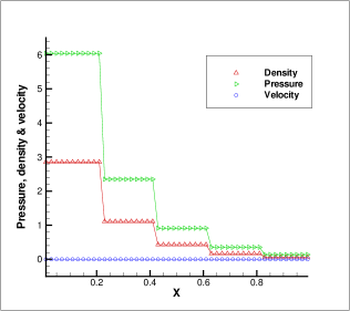
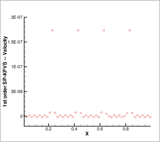
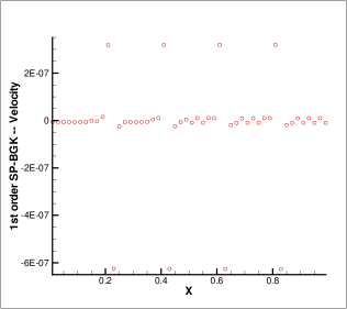
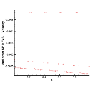
Figure 7: The first figure shows the Density, pressure and velocity distributions calculated by $2^{nd}$ order SP-BGK for isolated gravitational system with adiabatic wall. Other figures are velocity distributions in this test case.

After a long time ($t=1000$), the flow distributions settle down into a piecewise constant state which are shown in the fist picture of fig. 7, where the symbols are the numerical solutions and the solid lines are the exact hydrostatic solutions. The velocity distributions are also shown in fig. 7. For the $1^{st}$ order schemes, the oscillation of velocity around zero is on the order of $10^{-7}$. This is mainly caused by the error in numerical integrations because there is no exact solution for most integrals in Eq.(92)-(95). In fact, the precision of numerical integration for the integrals is on the order of $10^{-6}\sim 10^{-7}$. Since the potential jumps are large and the high order scheme uses more integral evaluations, the velocity distribution calculated by $2^{nd}$ order scheme is a little bit worse than the 1st-order ones. If a better accuracy can be achieved for the numerical evaluation of the integrals, the velocity error can be further reduced to machine zero.

6.3 Perturbation of the 1D isothermal equilibrium solution

This test case is from LeVeque and Bale’s paper [4]. We consider an ideal gas with $\gamma=1.4$ on an initial isothermal hydrostatic state,

$$\rho_{0}(x)=p_{0}(x)=e^{-x},\textrm{ and }U_{0}(x)=0,$$

for $x\in[0,1]$. Initially, the pressure is perturbed by

$$p(x,t=0)=p_{0}(x)+\eta e^{\alpha(x-x_{0})^{2}},$$

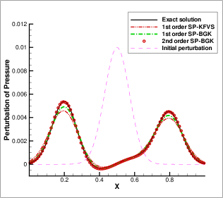
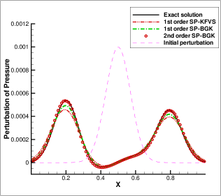
Figure 8: Perturbation of pressure on an isothermal equilibrium solution. Left: $\eta=0.01$; right: $\eta=0.001$.

where $\alpha=100$, $x_{0}=0.5$ and $\eta$ is the amplitude of the perturbation. The gravitational field is the same as in example 6.1. The computation is conducted with $100$ grid points in the whole domain and stops at time $t=0.25$. Fig. 8, show the results from SP-KFVS and SP-BGK schemes, where SP-KFVS has larger numerical dissipation than SP-BGK scheme. The results calculated by the $2^{nd}$ order SP-BGK scheme matches the exact solution very well.

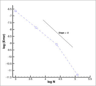
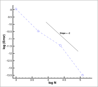
Figure 9: Convergency rate of the $2^{nd}$-order SP-BGK scheme for perturbation of pressure on an isothermal equilibrium solution with $\eta=0.01$ on the left figure, and $\eta=0.001$ on the right figure.

Also in fig. 9, we show the convergency rate of our $2^{nd}$-order SP-BGK scheme, where the number of cells is N and the error is the $L^{\infty}$ error. From the figures, we can conclude our $2^{nd}$-order SP-BGK scheme has a 2nd-order accuracy even with the modeling of piecewise constant potential.

6.4 One-dimension gas falling into a fixed external potential.

This case is taken from the paper by Slyz and Prendergast [9] to investigate the numerical accuracy of the BGK scheme. The gas is initially stationary ($U=0$) and homogeneous ($\rho=1$, $e=1$, where $e$ is the internal energy). The gravitational potential has the form of a sine wave,

$$\phi=-\phi_{0}\frac{L}{2\pi}\sin\frac{2\pi x}{L},$$

where $L=64$ is the length of the computational domain and $\phi_{0}=0.02$. The ratio of the specific heat $\gamma=5/3$. The periodic boundary conditions are implemented in this system. Simulation results are presented with $\Delta x=1$ and at the output time $t=250000$ (more than 500000 time steps). After the initial transition, the system is expected to reach an isothermal hydrostatic distribution, where the temperature settles to a constant with zero velocity, i.e.,

$$T(x,t)=T_{0},\textrm{ and }U=0.$$

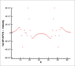
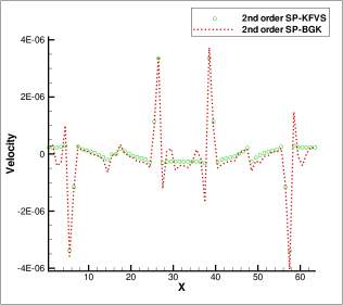
Figure 11: Velocity distributions for gas falling into a fixed external potential in 1-D case. The exact solution should have a zero velocity. The error is due to the numerical integration, e.g., $\int_{-\infty}^{0}g(u)(-\frac{u}{\sqrt{u^{2}+U_{c}^{2}}})\mathrm{d}u$, where there is no analytic solution.

The velocity and temperature distributions computed by different symplecticity preserving schemes are shown in fig. 11,  12. The numerical error is smaller than that in [10]. Moreover, the results can be further improved if a better numerical integration for the integral evaluation can be adopted.

6.5 Rayleigh-Taylor instability.

This test case also comes from [4]. Consider an isothermal equilibrium idea gas ($\gamma=1.4$) in a 2D polar coordinate $(r,\theta)$,

$$\rho_{0}(r)=e^{-\alpha(r+r_{0})},\,p_{0}(r)=\frac{1.5}{\alpha}e^{-\alpha(r+r_{0})},\,U_{0}=0,$$

where

$$\left\{\begin{array}[]{lr}\alpha=2.68,\,r_{0}=0.258&\text{for}\,r\leq r_{1},\\ \\ \alpha=5.53,\,r_{0}=-0.308&\text{for}\,r>r_{1},\end{array}\right.\,\text{and}\,\left\{\begin{array}[]{lr}r_{1}=0.6(1+0.02\cos(20\theta))&\text{for}\,density,\\ \\ r_{1}=0.62324965&\text{for}\,pressure,\end{array}\right.$$

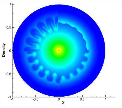
Figure 13: Rayleigh-Taylor instability with gravitational field directed radially inward. Density contours at time $t=0,0.8,1.4,2.0$ are shown in the four quadrants, starting with the initial data in the upper right corner and progressing clockwise.

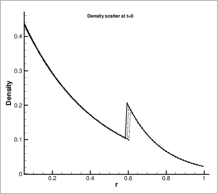
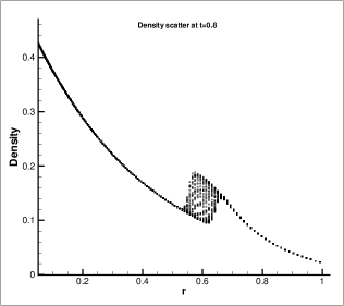
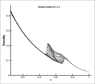
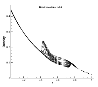
Figure 14: Scatter plots of the density in the cell vs. the distance of the cell center from the origin.

The potential satisfies $-\nabla\phi(r)=1.5$. The time evolutions of the density distributions at times $t=0,0.8,1.4$ and $2.0$ are shown in fig. 13. Fig. 14 shows a scatter plot of the density as a function of the radius. These figures clearly show that the hydrostatic solution can be well kept and the flow motion is limited around the unstable interface.

7 Conclusion

In this paper, based on the Liouville’s theorem and symplecticity-preserving property of a Hamiltonian flow, a well-balanced gas-kinetic BGK scheme (SP-BGK) has been developed for a hydrodynamic system under gravitational field with the modeling of piecewise constant potentials. As shown in the paper, in order to design such a scheme, the equilibrium state used has to be an exact Maxwellian distribution function. At the same time, the physical mechanism of particle transport across a potential barrier has to be explicitly followed in the equilibrium states modeling and the flux evaluation. As far as we know, the method presented in this paper is the first exact well-balanced scheme for the Navier-Stokes equations under gravitational field. At the same time, the particle transport mechanism across a potential jump in the current kinetic formulation follows the physical principles closely, which is valid under any general physical situation. Both the shock capturing and well-balanced properties are automatically obtained under the corresponding physical conditions. Mathematically, it has been proved that the SP-BGK method is a well-balanced scheme which could keep the hydrostatic state forever. In this paper, the design of the well-balanced scheme comes from the first principles of physics, instead of using the well-balanced condition as the starting point in the design of such a scheme.

Appendix

Formulae in the two-dimensional case:

1. Equilibrium states

Case 1. $\phi_{j}<\phi_{j+1}$, define $U_{c}=\sqrt{2(\phi_{j+1}-\phi_{j})}$.

$$\begin{array}[]{l}\quad W_{j+1/2}^{l}=\iiint^{+\infty}_{0}f_{j}(x_{j+1/2},0,u,v,\xi)\left(\begin{array}[]{c}1\\ u\\ v\\ \frac{1}{2}(u^{2}+v^{2}+\xi^{2})\end{array}\right)\mathrm{d}u\,\mathrm{d}v\,\mathrm{d}\xi\\ \\ \quad+\iiint^{U_{c}}_{0}f_{j}(x_{j+1/2},0,u,v,\xi)\left(\begin{array}[]{c}1\\ -u\\ v\\ \frac{1}{2}(u^{2}+\xi^{2})\end{array}\right)\mathrm{d}u\,\mathrm{d}v\,\mathrm{d}\xi\\ \\ \quad+\iiint_{-\infty}^{0}f_{j+1}(x_{j+1/2},0,u,v,\xi)\left(\begin{array}[]{c}-\frac{u}{\sqrt{u^{2}+v^{2}+U_{c}^{2}}}\\ u\\ -\frac{uv}{\sqrt{u^{2}+U_{c}^{2}}}\\ \frac{1}{2}(-u\sqrt{u^{2}+U_{c}^{2}}-\frac{uv^{2}}{\sqrt{u^{2}+U_{c}^{2}}}-\frac{u}{\sqrt{u^{2}+U_{c}^{2}}}\xi^{2})\end{array}\right)\mathrm{d}u\,\mathrm{d}v\,\mathrm{d}\xi.\end{array}$$ (80)

$$\begin{array}[]{l}W_{j+1/2}^{r}=\iiint^{+\infty}_{U_{c}}f_{j}(x_{j+1/2},0,u,v,\xi)\left(\begin{array}[]{c}\frac{u}{\sqrt{u^{2}-U_{c}^{2}}}\\ u\\ \frac{uv}{\sqrt{u^{2}-U_{c}^{2}}}\\ \frac{1}{2}(u\sqrt{u^{2}-U_{c}^{2}}+\frac{uv^{2}}{\sqrt{u^{2}-U_{c}^{2}}}+\frac{u}{\sqrt{u^{2}-U_{c}^{2}}}\xi^{2})\end{array}\right)\mathrm{d}u\,\mathrm{d}v\,\mathrm{d}\xi\\ \\ \quad+\iiint_{-\infty}^{0}f_{j+1}(x_{j+1/2},0,u,v,\xi)\left(\begin{array}[]{c}1\\ u\\ v\\ \frac{1}{2}(u^{2}+v^{2}+\xi^{2})\end{array}\right)\mathrm{d}u\,\mathrm{d}v\,\mathrm{d}\xi.\end{array}$$ (81)

Case 2. $\phi_{j}>\phi_{j+1}$, define $U_{c}=\sqrt{2(\phi_{j}-\phi_{j+1})}$.

$$\begin{array}[]{l}W_{j+1/2}^{l}=\iiint^{+\infty}_{0}f_{j}(x_{j+1/2},0,u,\xi)\left(\begin{array}[]{c}1\\ u\\ v\\ \frac{1}{2}(u^{2}+v^{2}+\xi^{2})\end{array}\right)\mathrm{d}u\,\mathrm{d}v\,\mathrm{d}\xi\\ \\ \quad+\iiint_{-\infty}^{-U_{c}}f_{j+1}(x_{j+1/2},0,u,\xi)\left(\begin{array}[]{c}-\frac{u}{\sqrt{u^{2}-U_{c}^{2}}}\\ u\\ -\frac{uv}{\sqrt{u^{2}-U_{c}^{2}}}\\ \frac{1}{2}(-u\sqrt{u^{2}-U_{c}^{2}}-\frac{uv^{2}}{\sqrt{u^{2}-U_{c}^{2}}}-\frac{u}{\sqrt{u^{2}-U_{c}^{2}}}\xi^{2})\end{array}\right)\mathrm{d}u\,\mathrm{d}v\,\mathrm{d}\xi.\end{array}$$ (82)

$$\begin{array}[]{l}W_{j+1/2}^{r}=\iiint^{+\infty}_{0}f_{j}(x_{j+1/2},0,u,\xi)\left(\begin{array}[]{c}\frac{u}{\sqrt{u^{2}+U_{c}^{2}}}\\ u\\ \frac{uv}{\sqrt{u^{2}+U_{c}^{2}}}\\ \frac{1}{2}(u\sqrt{u^{2}+U_{c}^{2}}+\frac{uv^{2}}{\sqrt{u^{2}+U_{c}^{2}}}+\frac{u}{\sqrt{u^{2}+U_{c}^{2}}}\xi^{2})\end{array}\right)\mathrm{d}u\,\mathrm{d}v\,\mathrm{d}\xi\\ \\ \quad+\iiint_{-U_{c}}^{0}f_{j+1}(x_{j+1/2},0,u,\xi)\left(\begin{array}[]{c}1\\ -u\\ v\\ \frac{1}{2}(u^{2}+v^{2}+\xi^{2})\end{array}\right)\mathrm{d}u\,\mathrm{d}v\,\mathrm{d}\xi\\ \\ \quad+\iiint_{-\infty}^{0}f_{j+1}(x_{j+1/2},0,u,\xi)\left(\begin{array}[]{c}1\\ u\\ v\\ \frac{1}{2}(u^{2}+v^{2}+\xi^{2})\end{array}\right)\mathrm{d}u\,\mathrm{d}v\,\mathrm{d}\xi.\end{array}$$ (83)

2. Fluxes

Case 1. $\phi_{j}<\phi_{j+1}$, define $U_{c}=\sqrt{2(\phi_{j+1}-\phi_{j})}$.

$$\begin{array}[]{l}F^{l}_{j+1/2}(t)=\iiint^{+\infty}_{0}f_{j}(x_{j+1/2},t,u,\xi)\left(\begin{array}[]{c}u\\ u^{2}\\ uv\\ \frac{1}{2}(u^{3}+uv^{2}+u\xi^{2})\end{array}\right)\mathrm{d}u\,\mathrm{d}v\,\mathrm{d}\xi\\ \\ \qquad\qquad\quad+\iiint^{U_{c}}_{0}f_{j}(x_{j+1/2},t,u,\xi)\left(\begin{array}[]{c}-u\\ u^{2}\\ -uv\\ \frac{1}{2}(-u^{3}-uv^{2}-u\xi^{2})\end{array}\right)\mathrm{d}u\,\mathrm{d}v\,\mathrm{d}\xi\\ \\ \qquad\qquad\quad+\iiint_{-\infty}^{0}f_{j+1}(x_{j+1/2},t,u,\xi)\left(\begin{array}[]{c}u\\ -u\sqrt{u^{2}+U_{c}^{2}}\\ uv\\ \frac{1}{2}(u(u^{2}+U_{c}^{2})+uv^{2}+u\xi^{2})\end{array}\right)\mathrm{d}u\,\mathrm{d}v\,\mathrm{d}\xi.\end{array}$$ (84)

$$\begin{array}[]{l}F^{r}_{j+1/2}(t)=\iiint^{+\infty}_{U_{c}}f_{j}(x_{j+1/2},t,u,\xi)\left(\begin{array}[]{c}u\\ u\sqrt{u^{2}-U_{c}^{2}}\\ uv\\ \frac{1}{2}(u(u^{2}-U_{c}^{2})+uv^{2}+u\xi^{2})\end{array}\right)\mathrm{d}u\,\mathrm{d}v\,\mathrm{d}\xi\\ \\ \qquad\qquad\quad+\iiint_{-\infty}^{0}f_{j+1}(x_{j+1/2},t,u,\xi)\left(\begin{array}[]{c}u\\ u^{2}\\ uv\\ \frac{1}{2}(u^{3}+uv^{2}+u\xi^{2})\end{array}\right)\mathrm{d}u\,\mathrm{d}v\,\mathrm{d}\xi.\end{array}$$ (85)

Case 2. $\phi_{j}>\phi_{j+1}$, define $U_{c}=\sqrt{2(\phi_{j}-\phi_{j+1})}$.

$$\begin{array}[]{l}F^{l}_{j+1/2}(t)=\iiint^{+\infty}_{0}f_{j}(x_{j+1/2},t,u,\xi)\left(\begin{array}[]{c}u\\ u^{2}\\ uv\\ \frac{1}{2}(u^{3}+uv^{2}+u\xi^{2})\end{array}\right)\mathrm{d}u\,\mathrm{d}v\,\mathrm{d}\xi\\ \\ \qquad\qquad\quad+\iiint_{-\infty}^{-U_{c}}f_{j+1}(x_{j+1/2},t,u,\xi)\left(\begin{array}[]{c}u\\ -u\sqrt{u^{2}-U_{c}^{2}}\\ uv\\ \frac{1}{2}(u(u^{2}-U_{c}^{2})+uv^{2}+u\xi^{2})\end{array}\right)\mathrm{d}u\,\mathrm{d}v\,\mathrm{d}\xi.\end{array}$$ (86)

$$\begin{array}[]{l}F^{r}_{j+1/2}(t)=\iiint^{+\infty}_{0}f_{j}(x_{j+1/2},t,u,\xi)\left(\begin{array}[]{c}u\\ u\sqrt{u^{2}+U_{c}^{2}}\\ uv\\ \frac{1}{2}(u(u^{2}+U_{c}^{2})+uv^{2}+u\xi^{2})\end{array}\right)\mathrm{d}u\,\mathrm{d}v\,\mathrm{d}\xi\\ \\ \qquad\qquad\quad+\iiint_{-U_{c}}^{0}f_{j+1}(x_{j+1/2},t,u,\xi)\left(\begin{array}[]{c}-u\\ u^{2}\\ -uv\\ \frac{1}{2}(-u^{3}-uv^{2}-u\xi^{2})\end{array}\right)\mathrm{d}u\,\mathrm{d}v\,\mathrm{d}\xi\\ \\ \qquad\qquad\quad+\iiint_{-\infty}^{0}f_{j+1}(x_{j+1/2},t,u,\xi)\left(\begin{array}[]{c}u\\ u^{2}\\ uv\\ \frac{1}{2}(u^{3}+uv^{2}+u\xi^{2})\end{array}\right)\mathrm{d}u\,\mathrm{d}v\,\mathrm{d}\xi.\end{array}$$ (87)

Formulae in the one-dimensional case:

1. Equilibrium states:

Case 1. $\phi_{j}<\phi_{j+1}$, define $U_{c}=\sqrt{2(\phi_{j+1}-\phi_{j})}$.

$$\begin{array}[]{l}W_{j+1/2}^{l}=\int\int^{+\infty}_{0}f_{j}(x_{j+1/2},0,u,\xi)\left(\begin{array}[]{c}1\\ u\\ \frac{1}{2}(u^{2}+\xi^{2})\end{array}\right)\mathrm{d}u\,\mathrm{d}\xi\\ \\ \qquad\qquad+\int\int^{U_{c}}_{0}f_{j}(x_{j+1/2},0,u,\xi)\left(\begin{array}[]{c}1\\ -u\\ \frac{1}{2}(u^{2}+\xi^{2})\end{array}\right)\mathrm{d}u\,\mathrm{d}\xi\\ \\ \qquad\qquad+\int\int_{-\infty}^{0}f_{j+1}(x_{j+1/2},0,u,\xi)\left(\begin{array}[]{c}-\frac{u}{\sqrt{u^{2}+U_{c}^{2}}}\\ u\\ \frac{1}{2}(-u\sqrt{u^{2}+U_{c}^{2}}-\frac{u}{\sqrt{u^{2}+U_{c}^{2}}}\xi^{2})\end{array}\right)\mathrm{d}u\,\mathrm{d}\xi.\end{array}$$ (88)

$$\begin{array}[]{l}W_{j+1/2}^{r}=\int\int^{+\infty}_{U_{c}}f_{j}(x_{j+1/2},0,u,\xi)\left(\begin{array}[]{c}\frac{u}{\sqrt{u^{2}-U_{c}^{2}}}\\ u\\ \frac{1}{2}(u\sqrt{u^{2}-U_{c}^{2}}+\frac{u}{\sqrt{u^{2}-U_{c}^{2}}}\xi^{2})\end{array}\right)\mathrm{d}u\,\mathrm{d}\xi\\ \\ \qquad\qquad+\int\int_{-\infty}^{0}f_{j+1}(x_{j+1/2},0,u,\xi)\left(\begin{array}[]{c}1\\ u\\ \frac{1}{2}(u^{2}+\xi^{2})\end{array}\right)\mathrm{d}u\,\mathrm{d}\xi.\end{array}$$ (89)

Case 2. $\phi_{j}>\phi_{j+1}$, define $U_{c}=\sqrt{2(\phi_{j}-\phi_{j+1})}$.

$$\begin{array}[]{l}W_{j+1/2}^{l}=\int\int^{+\infty}_{0}f_{j}(x_{j+1/2},0,u,\xi)\left(\begin{array}[]{c}1\\ u\\ \frac{1}{2}(u^{2}+\xi^{2})\end{array}\right)\mathrm{d}u\,\mathrm{d}\xi\\ \\ \qquad\qquad+\int\int_{-\infty}^{-U_{c}}f_{j+1}(x_{j+1/2},0,u,\xi)\left(\begin{array}[]{c}-\frac{u}{\sqrt{u^{2}-U_{c}^{2}}}\\ u\\ \frac{1}{2}(-u\sqrt{u^{2}-U_{c}^{2}}-\frac{u}{\sqrt{u^{2}-U_{c}^{2}}}\xi^{2})\end{array}\right)\mathrm{d}u\,\mathrm{d}\xi.\end{array}$$ (90)

$$\begin{array}[]{l}W_{j+1/2}^{r}=\int\int^{+\infty}_{0}f_{j}(x_{j+1/2},0,u,\xi)\left(\begin{array}[]{c}\frac{u}{\sqrt{u^{2}+U_{c}^{2}}}\\ u\\ \frac{1}{2}(u\sqrt{u^{2}+U_{c}^{2}}+\frac{u}{\sqrt{u^{2}+U_{c}^{2}}}\xi^{2})\end{array}\right)\mathrm{d}u\,\mathrm{d}\xi\\ \\ \qquad\qquad+\int\int_{-U_{c}}^{0}f_{j+1}(x_{j+1/2},0,u,\xi)\left(\begin{array}[]{c}1\\ -u\\ \frac{1}{2}(u^{2}+\xi^{2})\end{array}\right)\mathrm{d}u\,\mathrm{d}\xi\\ \\ \qquad\qquad+\int\int_{-\infty}^{0}f_{j+1}(x_{j+1/2},0,u,\xi)\left(\begin{array}[]{c}1\\ u\\ \frac{1}{2}(u^{2}+\xi^{2})\end{array}\right)\mathrm{d}u\,\mathrm{d}\xi.\end{array}$$ (91)

2. Fluxes:

Case 1. $\phi_{j}<\phi_{j+1}$, define $U_{c}=\sqrt{2(\phi_{j+1}-\phi_{j})}$.

$$\begin{array}[]{l}F^{l}_{j+1/2}(t)=\int\int^{+\infty}_{0}f_{j}(x_{j+1/2},t,u,\xi)\left(\begin{array}[]{c}u\\ u^{2}\\ \frac{1}{2}(u^{3}+u\xi^{2})\end{array}\right)\mathrm{d}u\,\mathrm{d}\xi\\ \\ \qquad\qquad\quad+\int\int^{U_{c}}_{0}f_{j}(x_{j+1/2},t,u,\xi)\left(\begin{array}[]{c}-u\\ u^{2}\\ \frac{1}{2}(-u^{3}-u\xi^{2})\end{array}\right)\mathrm{d}u\,\mathrm{d}\xi\\ \\ \qquad\qquad\quad+\int\int_{-\infty}^{0}f_{j+1}(x_{j+1/2},t,u,\xi)\left(\begin{array}[]{c}u\\ -u\sqrt{u^{2}+U_{c}^{2}}\\ \frac{1}{2}(u(u^{2}+U_{c}^{2})+u\xi^{2})\end{array}\right)\mathrm{d}u\,\mathrm{d}\xi.\end{array}$$ (92)

$$\begin{array}[]{l}F^{r}_{j+1/2}(t)=\int\int^{+\infty}_{U_{c}}f_{j}(x_{j+1/2},t,u,\xi)\left(\begin{array}[]{c}u\\ u\sqrt{u^{2}-U_{c}^{2}}\\ \frac{1}{2}(u(u^{2}-U_{c}^{2})+u\xi^{2})\end{array}\right)\mathrm{d}u\,\mathrm{d}\xi\\ \\ \qquad\qquad\quad+\int\int_{-\infty}^{0}f_{j+1}(x_{j+1/2},t,u,\xi)\left(\begin{array}[]{c}u\\ u^{2}\\ \frac{1}{2}(u^{3}+u\xi^{2})\end{array}\right)\mathrm{d}u\,\mathrm{d}\xi.\end{array}$$ (93)

Case 2. $\phi_{j}>\phi_{j+1}$, define $U_{c}=\sqrt{2(\phi_{j}-\phi_{j+1})}$.

$$\begin{array}[]{l}F^{l}_{j+1/2}(t)=\int\int^{+\infty}_{0}f_{j}(x_{j+1/2},t,u,\xi)\left(\begin{array}[]{c}u\\ u^{2}\\ \frac{1}{2}(u^{3}+u\xi^{2})\end{array}\right)\mathrm{d}u\,\mathrm{d}\xi\\ \\ \qquad\qquad\quad+\int\int_{-\infty}^{-U_{c}}f_{j+1}(x_{j+1/2},t,u,\xi)\left(\begin{array}[]{c}u\\ -u\sqrt{u^{2}-U_{c}^{2}}\\ \frac{1}{2}(u(u^{2}-U_{c}^{2})+u\xi^{2})\end{array}\right)\mathrm{d}u\,\mathrm{d}\xi.\end{array}$$ (94)

$$\begin{array}[]{l}F^{r}_{j+1/2}(t)=\int\int^{+\infty}_{0}f_{j}(x_{j+1/2},t,u,\xi)\left(\begin{array}[]{c}u\\ u\sqrt{u^{2}+U_{c}^{2}}\\ \frac{1}{2}(u(u^{2}+U_{c}^{2})+u\xi^{2})\end{array}\right)\mathrm{d}u\,\mathrm{d}\xi\\ \\ \qquad\qquad\quad+\int\int_{-U_{c}}^{0}f_{j+1}(x_{j+1/2},t,u,\xi)\left(\begin{array}[]{c}-u\\ u^{2}\\ \frac{1}{2}(-u^{3}-u\xi^{2})\end{array}\right)\mathrm{d}u\,\mathrm{d}\xi\\ \\ \qquad\qquad\quad+\int\int_{-\infty}^{0}f_{j+1}(x_{j+1/2},t,u,\xi)\left(\begin{array}[]{c}u\\ u^{2}\\ \frac{1}{2}(u^{3}+u\xi^{2})\end{array}\right)\mathrm{d}u\,\mathrm{d}\xi.\end{array}$$ (95)

Remarks on the integral evaluation: in the above formulae, there are many integrals which can not be analytically evaluated, e.g., $\int_{-\infty}^{0}f_{j+1}(-\frac{u}{\sqrt{u^{2}+U_{c}^{2}}})\mathrm{d}u$. Therefore, a numerical integration method in [7] has been used.

References

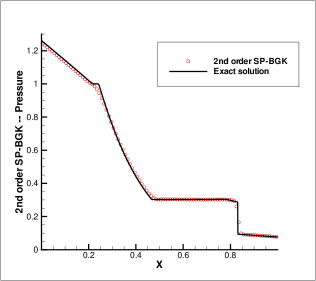
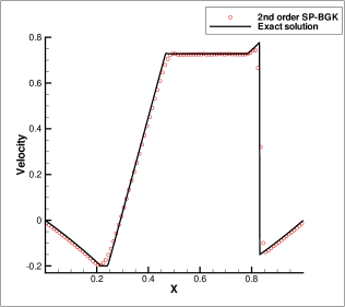
Figure 6: Pressure and velocity distributions for the shock tube problem under gravitational field.

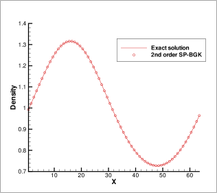
Figure 10: Density distribution calculated by $2^{nd}$-order SP-BGK for gas falling into a fixed external potential in 1-D case.

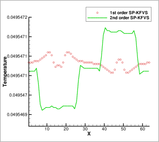
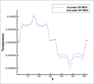
Figure 12: Temperature distributions for gas falling into a fixed external potential in 1-D case.

References

- [1] P.L. Bhatnagar, E.P. Gross, and M. Krook, A Model for Collision Processes in Gases I: Small Amplitude Processes in Charged and Neutral One-Component Systems, Phys. Rev., 94 (1954), pp. 511-525.
- [2] N. Botta, R. Klein, S. Langenberg, and S. Lutzenkirchen, Well-balanced finite volume methods for nearly hydrostatic flows, J. Comput. Phys. 196 (2004), pp. 539–565.
- [3] C.S. Frenk, et al., The Santa Barbara cluster comparison project: a comparison of cosmological hydrodynamics solutions, The Astrophy. J, 525 (1999), pp. 554-582.
- [4] R.J. LeVeque and D.S. Bale, Wave propagation methods for conservation laws with source terms, Proc. 7th International Conference on Hyperbolic Problems, Zurich, February (1998).
- [5] R.J. LeVeque, Numerical Methods for Conservation Laws, Birkhäuser Verlag, Basel, 1992, pp. 122-135.
- [6] B. Perthame and C. Simeoni, A kinetic scheme for the Saint-Venant system with a source term,CALCOLO, 38 (2001), pp. 201-231.
- [7] W.H. Press, B.P. Flannery, S.A. Teukolsky, and W.T. Vetterling, Numerical Recipes, Cambridge University Press (1989).
- [8] D. Ryu, J.P. Ostriker, H. Kang, and R. Cen, A cosmological hydrodynamic code based on the total variation diminishing scheme, Astrophy. J. 414 (1993), pp. 1-19.
- [9] A. Slyz, K.H. Prendergast, Time-independent gravitational fields in the BGK scheme for hydrodynamics, Astron. Astrophys. Suppl. Ser. 139 (1999), pp. 199-217.
- [10] C.L. Tian, K. Xu, K.L. Chan, and L.C. Deng, A three-dimensional multidimensional gas kinetic scheme for the Navier-Stokes equations under gravitational fields, J. Comput. Phys., vol. 226 (2007), pp. 2003-2027.
- [11] K. Xu, Gas-Kinetic Schemes for Unsteady Compressible Flow Simulations, von Karman Institute report, (1998-03).
- [12] K. Xu, A gas-kinetic BGK scheme for the Navier-Stokes equations, and its connection with artificial dissipation and Godunov method, J. Comput. Phys., vol. 171 (2001), pp. 289-335.
- [13] K. Xu, A well-balanced gas-kinetic scheme for the shallow-water equations with source terms, J. Comput. Phys., 178 (2002), pp. 533–562.
- [14] K. Xu, J. Luo, and S.Z. Chen, A well-balanced kinetic scheme for gas dynamic equations under gravitational field, to appear in Advances in Applied Mathematics and Mechanics, 2010.
- [15] M. Zingale, et. al., Mapping initial hydrostatic models in Godunov codes, Astro. Phys. J. Supple, 143 (2002), pp. 539-565.