$\mathbf{K^{0}-\bar{K}^{0}}$ Mixing Beyond the SM from $\mathbf{N_{f}=2}$ tmQCD

Abstract:

We present preliminary results on the of neutral kaon oscillations in extensions of the Standard Model. Using $N_{f}=2$ maximally twisted sea quarks and Osterwalder-Seiler valence quarks, we achieve both O(a)-improvement and continuum-like renormalization pattern for the relevant four-fermion operators. We perform simulations at three values of the lattice spacing and extrapolate/interpolate our results to the continuum limit and physical light/strange quark mass. The calculation of the renormalization constants of the complete operator basis is performed non- perturbatively in the RI-MOM scheme.

1 Introductory Remarks and Calculation Setup

Flavour Changing Neutral Currents (FCNC) and CP violation may furnish useful information on the impact of models defined beyond the standard model (BSM). In various BSM models (like for example the supersymmetric ones) there appears the possibility for $\Delta S=2$ processes at one loop, even mediated by the strong interactions. These effects are thus potentially large. The computation of the relevant matrix elements of the effective Hamiltonian in combination with the experimental value of $\varepsilon_{K}$ offers the chance to constrain the values of the model parameters (like for instance the off-diagonal terms of the squark mass matrix in supersymmetric models [1]) which enter explicitly in the Wilson coefficients.

In all the BSM models the effective Hamiltonian relevant for the $\Delta S=2$ processes takes the general form

$${\cal H}_{\rm{eff}}^{\Delta S=2}=\sum_{i=1}^{5}C_{i}(\mu){\cal O}_{i}+\sum_{i=1}^{3}\tilde{C}_{i}(\mu)\tilde{{\cal O}}_{i}$$ (1)

where the operators ${\cal O}_{i}$ are defined by

$${\cal O}_{1} = [\bar{s}^{a}\gamma_{\mu}(1-\gamma_{5})d^{a}][\bar{s}^{b}\gamma_{\mu}(1-\gamma_{5})d^{b}],$$

$${\cal O}_{2} = [\bar{s}^{a}(1-\gamma_{5})d^{a}][\bar{s}^{b}(1-\gamma_{5})d^{b}],~{}~{}~{}~{}~{}~{}~{}~{}{\cal O}_{3}=[\bar{s}^{a}(1-\gamma_{5})d^{b}][\bar{s}^{b}(1-\gamma_{5})d^{a}],$$

$${\cal O}_{4} = [\bar{s}^{a}(1-\gamma_{5})d^{a}][\bar{s}^{b}(1+\gamma_{5})d^{b}],~{}~{}~{}~{}~{}~{}~{}~{}{\cal O}_{5}=[\bar{s}^{a}(1-\gamma_{5})d^{b}][\bar{s}^{b}(1+\gamma_{5})d^{a}]$$ (2)

We note that in the SM case only the operator ${\cal O}_{1}$ contributes. The parity-even parts of the operators

$$\tilde{{\cal O}}_{1} = [\bar{s}^{a}\gamma_{\mu}(1+\gamma_{5})d^{a}][\bar{s}^{b}\gamma_{\mu}(1+\gamma_{5})d^{b}],$$

$$\tilde{{\cal O}}_{2} = [\bar{s}^{a}(1+\gamma_{5})d^{a}][\bar{s}^{b}(1+\gamma_{5})d^{b}],~{}~{}~{}~{}~{}~{}~{}~{}\tilde{{\cal O}}_{3}=[\bar{s}^{a}(1+\gamma_{5})d^{b}][\bar{s}^{b}(1+\gamma_{5})d^{a}]$$ (3)

coincide with those of the operators ${\cal O}_{i}$. Therefore, due the parity conservation of the strong interactions only the parity-even contributions of the operators ${\cal O}_{i}$ need to be calculated. Defining a basis of the parity even operators as follows

$$O^{VV} = (\bar{s}\gamma_{\mu}d)(\bar{s}\gamma_{\mu}d),~{}~{}~{}~{}~{}~{}~{}~{}O^{AA}=(\bar{s}\gamma_{\mu}\gamma_{5}d)(\bar{s}\gamma_{\mu}\gamma_{5}d),$$

$$O^{PP} = (\bar{s}\gamma_{5}d)(\bar{s}\gamma_{5}d),~{}~{}~{}~{}~{}~{}~{}~{}~{}\,O^{SS}=(\bar{s}d)(\bar{s}d),$$

$$O^{TT} = (\bar{s}\sigma_{\mu\nu}d)(\bar{s}\sigma_{\mu\nu}d)$$ (4)

through a Fierz transformation we obtain

$${\cal O}_{1} = (O^{VV}+O^{AA}),~{}~{}~{}~{}~{}~{}{\cal O}_{2}=(O^{SS}+O^{PP}),~{}~{}~{}~{}~{}~{}{\cal O}_{3}=-\frac{1}{2}(O^{SS}+O^{PP}-O^{TT}),$$

$${\cal O}_{4} = (O^{SS}-O^{PP}),~{}~{}~{}~{}~{}~{}~{}{\cal O}_{5}=-\frac{1}{2}(O^{VV}-O^{AA})$$ (5)

Up to now, lattice calculations have been presented in the quenched approximation ([2], [3], [4]) with the exception of a preliminary study of the bare matrix elements using unquenched simulations with 2+1 dynamical quarks [5].

Our lattice computations have been performed at three values of the lattice spacing using the $N_{f}=2$ dynamical quark configurations produced by the ETM collaboration [6]. ETMC dynamical configurations have been produced with the tree-level Symmanzik improved action in the gauge sector while the dynamical quarks have been regularized by employing the twisted mass (tm) formalism [7]. It has been demonstrated that with the condition at maximal twist this formalism provides automatic $O(a)$-improved physical quantities [8].

In the so called physical basis the fermion lattice action concerning the sea sector is written

$$S_{sea}^{\rm Mtm}=a^{4}\sum_{x}\bar{\psi}(x)\Big{\{}\frac{1}{2}\sum_{\mu}\gamma_{\mu}(\nabla_{\mu}+\nabla^{\ast}_{\mu})-i\gamma_{5}\tau^{3}\big{[}M_{\rm cr}-\frac{a}{2}\sum_{\mu}\nabla^{\ast}_{\mu}\nabla_{\mu}\big{]}+\mu_{sea}\Big{\}}\psi(x)$$ (6)

where the Wilson’s $r$ parameter has been set to unity, $\psi(x)$ is the quark flavour doublet, $\nabla_{\mu}$ and $\nabla_{\mu}^{\ast}$ are nearest-neighbour forward and backward lattice covariant derivatives, $\mu_{sea}$ is the (twisted) sea quark mass and $M_{\rm cr}$ the critical mass. It has been shown that the use of the tm regularization can simplify the renormalization pattern properties of the four-fermion operators (e.g. $B_{\rm{K}}$) [7, 9, 10]. Moreover, both $O(a)$ improvement and continuum-like operator renormalization pattern can be achieved introducing a valence quark action of the Osterwalder-Seiler type [11] by allowing for a replica of the down ($d$, $d^{\prime}$) and strange ($s$, $s^{\prime}$) flavours [12]. The valence quark action assumes the form

$$S_{val}=a^{4}\sum_{x}\sum_{f=d,d^{\prime},s,s^{\prime}}\bar{q}_{f}(x)\,\Big{\{}\frac{1}{2}\sum_{\mu}\gamma_{\mu}(\nabla_{\mu}+\nabla^{\ast}_{\mu})-i\gamma_{5}r_{f}\big{[}M_{\rm cr}-\frac{a}{2}\sum_{\mu}\nabla^{\ast}_{\mu}\nabla_{\mu}\big{]}+\mu_{f}\Big{\}}\,q_{f}(x)$$ (7)

with $-r_{s}=r_{d}=r_{d^{\prime}}=r_{s^{\prime}}=1$. Note that the field $q_{f}$ represents just one individual flavour. The four fermion operators of Eq. (1) can be written in general form as $O_{\Gamma\tilde{\Gamma}}=2\{[\bar{q_{1}}\Gamma q_{2}][\bar{q}_{3}\tilde{\Gamma}q_{4}]+(q_{2}\leftrightarrow q_{4})\}$ with $q_{1}$ and $q_{3}$ identified with the strange quark (by setting $\mu_{s}=\mu_{s^{\prime}}=\mu_{strange}$) and $q_{2}$ and $q_{4}$ identified with the down quark (by setting $\mu_{d}=\mu_{d^{\prime}}=\mu_{\ell}$); the interpolating fields for the external (anti)Kaon states are made up of a tm-quark pair ($\bar{d}\gamma_{5}s$, with $-r_{s}=r_{d}$) and a OS-quark pair ($\bar{d}^{\prime}\gamma_{5}s^{\prime}$, with $r_{d^{\prime}}=r_{s^{\prime}}$). This mixed action setup with maximally twisted Wilson-like quarks has been studied in detail in Ref. [12] and it has been demonstrated that it allows for an easy matching of sea and valence quark masses and leads to unitarity violations that vanish as $a^{2}$ as the continuum limit is approached. Moreover in the present computation the quark mass matching is incomplete because we are neglecting the sea strange quark (i.e. we work in a partially quenched set-up). A first test that the proposed method leads to $O(a)$ improved results was already performed in the calculation of $B_{K}$ with fully quenched quarks [13]. In a recent publication [14] our collaboration, using the OS-tm mixed action set-up, has presented an $O(a)$-improved computation of $B_{\rm{K}}$ with $N_{f}=2$ dynamical quarks. Using non-perturbative operator renormalisation and three values for the lattice spacing, the RGI value of $B_{\rm{K}}$ in the continuum limit is $B_{\rm{K}}^{\rm{RGI}}=0.729\pm 0.030$.

$\beta$		$a^{-4}(L^{3}\times T)$		$a\mu_{\ell}~{}=~{}a\mu_{sea}$		$a\mu_{\rm{``}s\rm{"}}$
3.80		$24^{3}\times 48$		0.0080 0.0110		0.0165, 0.0200, 0.0250
($a\sim 0.1~{}\mbox{fm}$)
3.90		$24^{3}\times 48$		0.0040, 0.0064		0.0150, 0.0220, 0.0270
				0.0085, 0.0100
”		$32^{3}\times 64$		0.0030, 0.0040		0.0150, 0.0220, 0.0270
($a\sim 0.085~{}\mbox{fm}$)
4.05		$32^{3}\times 64$		0.0030, 0.0060		0.0120, 0.0150, 0.0180
($a\sim 0.065~{}\mbox{fm}$)				0.0080

Table 1: Simulation details

In Table 1 we give the simulation details and the values of the sea and the valence quark masses at each value of the gauge coupling for the calculation presented in this work. The smallest sea quark mass corresponds to a pion of about 280 MeV for the case of $\beta=3.90$. For $\beta=4.05$ the lightest pion weighs 300 MeV while for $\beta=3.80$ the lowest pion mass is around 400 MeV. The largest sea quark mass for the three values of the lattice spacing is about half the strange quark mass. For the inversions in the valence sector we have made use of the stochastic method (one–end trick of Ref. [15]) in order to increase the statistical information. Propagator sources have been located at randomly chosen timeslices. For more details on the dynamical configurations and the stochastic method application see Ref. [16].

2 B-Parameters and Four-Fermion Matrix Elements

As it has been shown in [12], the discrete symmetries guarantee that in the OS-tm mixed action set-up the renormalisation of the four-fermion operators is continuum-like in the sense that the mixing between operators of different naive chirality is of order $O(a^{2})$ or higher. An equivalent view of the same property can be offered by the fact that in the (unphysical) tm-basis the parity-even part of each of the four fermion operators is mapped over its parity-odd counterpart. Then due to the CPS symmetries the parity odd operators have the same block-diagonal renormalisation matrix pattern both in the continuum and at finite value of the lattice spacing ([17], [18]).

The B-parameters for the operators (1) are defined as

$$\langle\bar{K}^{0}|{\cal O}_{1}(\mu)|K^{0}\rangle = B_{1}(\mu)\frac{8}{3}m_{K}^{2}f_{K}^{2}\equiv B_{K}(\mu)\frac{8}{3}m_{K}^{2}f_{K}^{2}$$

$$\langle\bar{K}^{0}|{\cal O}_{i}(\mu)|K^{0}\rangle = C_{i}B_{i}(\mu)\LSB\frac{m_{K}^{2}f_{K}}{m_{s}(\mu)+m_{d}(\mu)}\RSB^{2},$$

where $C_{i}=\{-5/3,1/3,2,2/3\},~{}~{}i=2,\ldots,5$. The matrix element of the operator ${\cal O}_{1}$ vanishes in the chiral limit while the matrix element of the operators ${\cal O}_{i}~{}i=2,\ldots,5$ get a non-zero value in the chiral limit. From the above equations it can be seen that the calculation of the $B_{i}$ parameters for $i=2,\ldots,5$ involves the calculation of the quark mass at the same scale $\mu$. In order to avoid any extra systematic uncertainties in the computation of the matrix elements due to the quark mass evaluation, it has been proposed the calculation of appropriate ratios of the four-fermion matrix elements ([2], [3]). Here, besides the calculation of the $B$ parameters, we also consider the following ratios

$$R_{i}=\Big{(}\frac{f_{K}^{2}}{m_{K}^{2}}\Big{)}_{\rm{exp}}\LSB\Big{(}\frac{m_{K}}{f_{K}}\Big{)}_{-r_{s}=r_{d}}\Big{(}\frac{m_{K}}{f_{K}}\Big{)}_{r_{d^{\prime}}=r_{s^{\prime}}}\frac{\ME{\bar{K}^{0}}{{\cal O}_{i}(\mu)}{K^{0}}}{\ME{\bar{K}^{0}}{{\cal O}_{1}(\mu)}{K^{0}}}\RSB~{}~{}~{}i=2,\ldots,5$$ (8)

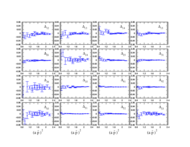
Figure 1: The off-diagonal off-block elements of the four-fermion RC-matrix operator, $\Delta{ij}$ , (for $\beta=3.90$) which take values compatible with zero.

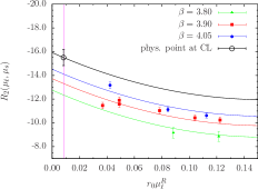
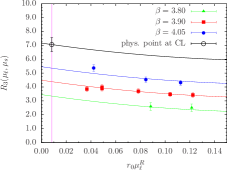
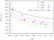
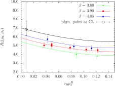
Figure 2: Combined fits of $R_{i}(\mu_{\ell},\mu_{s}),~{}i=2,\ldots,5$ with respect to the renormalised light quark mass, $r_{0}\mu_{\ell}^{R}$, in the $\overline{MS}$ scheme. The fit functions, shown here, are second order polynomial functions of the renormalised light quark mass with the addition of a term proportional to $a^{2}$.

The computation of the renormalisation constants (RCs) relevant for both the four-fermion and two-fermion operators has been performed in a non-perturbative way using the RI-MOM scheme following the strategies detailed in Refs. [19] and [20]. In Fig. 1 we show, for $\beta=3.90$, that all the off-diagonal off-block elements of the four-fermion RC-matrix operator, $\Delta_{ij}$, which are expected to vanish with the tm-OS mixed action setup, take values compatible with zero. In Fig. 2 we show the combined fits of $R_{i}(\mu_{\ell},\mu_{s}),~{}i=2,\ldots,5$ with respect to the renormalised light quark mass, $r_{0}\mu_{\ell}^{R}$, in the $\overline{MS}$ scheme.

fit function	$i$	$\frac{<{\cal O}_{i}>}{<{\cal O}_{1}>}$ (using $R_{i}$)	$\frac{<{\cal O}_{i}>}{<{\cal O}_{1}>}$ (using $B_{i}$)	$B_{i}$
quadratic	2	-15.5(1.0)	-17.1(1.5)	0.56(0.04)
	3	7.1(0.5)	8.7(0.9)	1.43(0.13)
	4	24.6(1.4)	27.9(2.5)	0.76(0.06)
	5	6.9(0.7)	7.6(1.2)	0.63(0.09)
linear	2	-15.0(0.6)	-17.1(1.2)	0.56(0.02)
	3	7.0(0.3)	8.8(0.6)	1.44(0.08)
	4	24.2(0.9)	27.8(1.8)	0.76(0.04)
	5	6.6(0.5)	7.5(0.7)	0.62(0.06)

Table 2: Preliminary results in the continuum limit for the B-parameters and the ratios $\frac{<{\cal O}_{i}>}{<{\cal O}_{1}>},~{}i=2,\ldots,5$. calculated at the physical point ($\mu_{d}$, $\mu_{s}$, $a=0$). All results are given in the $\overline{MS}$ scheme. The ratios of the operators’ matrix elements are estimated using either the direct (3rd column) or and the indirect method i.e. through the $B_{i}$ calculation (4th column) .

In Table 2 we present our preliminary results in the continuum limit and in the $\overline{MS}$ scheme for the B-parameters and the ratios $\frac{<{\cal O}_{i}>}{<{\cal O}_{1}>},~{}i=2,\ldots,5$ calculated at the physical point $(\mu_{d},\mu_{s})$. The ratios, $\frac{<{\cal O}_{i}>}{<{\cal O}_{1}>},~{}i=2,\ldots,5$, have been calculated either directly (through $R_{i}$) or using the $B_{i}$ estimates and the values of the u/d and strange quark mass [23]. The results are compatible within one or two standard deviations. We have tried fit functions using either a second or first order polynomial with respect to the light quark mass to which a term proportional to $a^{2}$ has been added; we do not notice a significant difference in the final continuum limit values. We should note that the use of a fit function containing a NLO logarithmic term leads to rather similar results with those obtained with a second order polynomial fit function.

References

• [1] M. Ciuchini et al. JHEP 9810 (1998) 008 [arXiv:hep-ph/9808328].
• [2] A. Donini, V. Gimenez, L. Giusti and G. Martinelli, Phys. Lett.  B 470 (1999) 233 [arXiv:hep-lat/9910017].
• [3] R. Babich et al. Phys. Rev.  D 74 (2006) 073009 [arXiv:hep-lat/0605016].
• [4] Y. Nakamura et al. PoS LAT2006 (2006) 089 [arXiv:hep-lat/0610075].
• [5] J. Wennekers [RBC Collaboration and QKQCD Collaboration], PoS LATTICE2008 (2008) 269 [arXiv:0810.1841 [hep-lat]].
• [6] R. Baron et al. [ETM Collaboration], JHEP 1008 (2010) 097 [arXiv:0911.5061 [hep-lat]].
• [7] ALPHA Collab., R. Frezzotti, P.A. Grassi, S. Sint and P. Weisz, JHEP08 (2001) 058 [hep-lat/0101001].
• [8] R. Frezzotti and G.C. Rossi, JHEP08 (2004) 007 [hep-lat/0306014].
• [9] ALPHA Collab., P. Dimopoulos et al. Nucl. Phys.B749 (2006) 69 [hep-ph/0601002];
ALPHA Collab., P. Dimopoulos et al. Nucl. Phys.  B 776 (2007) 258 [arXiv:hep-lat/0702017].
• [10] C. Pena, S. Sint and A.Vladikas, JHEP09 (2004)069 [hep-lat/0405028].
• [11] K. Osterwalder and E. Seiler, Annals Phys.  110 (1978) 440.
• [12] R. Frezzotti and G.C. Rossi, JHEP10 (2004) 070 [hep-lat/0407002].
• [13] ALPHA Collab., P. Dimopoulos, H. Simma and A. Vladikas, JHEP 0907 (2009) 007 [arXiv:0902.1074 [hep-lat]].
• [14] M. Constantinou et al. [ETM Collaboration], arXiv:1009.5606 [hep-lat].
• [15] M. Foster and C. Michael, Phys.Rev.D59 (1999) 074503 [hep-lat/9810021];
C. Mc Neile and C. Michael, Phys.Rev.D73 (2006) 074506 [hep-lat/0603007].
• [16] Ph. Boucaud et al. [ETM collaboration], Phys.Lett.B650 (2007) 304 [hep-lat/0701012];
Ph. Boucaud et al. [ETM collaboration], Comput. Phys. Commun.  179 (2008) 695 [arXiv:0803.0224 [hep-lat]].
• [17] C. Bernard, TASI Lectures 1989.
• [18] A. Donini et al, Eur. Phys. J.C10 1999 121 [hep-lat/9902030].
• [19] G. Martinelli et al. Nucl. Phys.B445 (1995) 81 [hep-lat/9411010].
• [20] M. Constantinou et al. [ETM Collaboration], JHEP 1008 (2010) 068 [arXiv:1004.1115 [hep-lat]].
• [21] D. Becirevic et al. JHEP05 (2003) 007 [hep-lat/0301020].
• [22] C. R. Allton et al. Phys. Lett.  B 453 (1999) 30 [arXiv:hep-lat/9806016].
• [23] B. Blossier et al. [ETM Collaboration], arXiv:1010.3659 [hep-lat]