Practical Statistics for the Voids Between Galaxies

The voids between galaxies are identified with the volumes of the Poisson Voronoi tessellation. Two new survival functions for the apparent radii of voids are derived. The sectional normalized area of the Poisson Voronoi tessellation is modelled by the Kiang function and by the exponential function. Two new survival functions with equivalent sectional radius are therefore derived; they represent an alternative to the survival function of voids between galaxies as given by the self-similar distribution. The spatial appearance of slices of the 2dF Galaxy Redshift Survey is simulated.
keywords
methods: statistical ; cosmology: observations; (cosmology): large-scale structure of the Universe

1 Introduction

The statistical analysis of the voids between galaxies is a field of research and the following catalogs have been explored: the two-degree Field Galaxy Redshift Survey (2dFGRS), see Patiri et al. (2006) and von Benda-Beckmann & Müller (2008), the Sloan Digital Sky Survey (SDSS), see Tikhonov (2007), and the combination of 2dFGRS and SDSS, see Tinker et al. (2008). The voids between galaxies are usually modelled by a survival function in the apparent radius as given by a modified exponential distribution, see (3) in von Benda-Beckmann & Müller (2008) or our Section 4; this fact is considered here a standard argument for comparison. The concept of Voronoi Diagrams dates back to the vortex theory applied to the solar system as developed in the 17th century, see Descartes (1644) and Figure 1 in Aurenhammer, F. and Klein, R. In : Sack, J.-R. (2000). The name is due to the two historical records by Voronoi (1907, 1908) and the applications to astrophysics beginning with  Kiang (1966). The Voronoi diagrams represent a model of the voids between galaxies, see van de Weygaert & Icke (1989), Pierre (1990), Barrow & Coles (1990), Coles (1991), van de Weygaert (1991), van de Weygaert (1991), Zaninetti (1991), Ikeuchi & Turner (1991), Subba Rao & Szalay (1992), van de Weygaert (1994), Goldwirth et al. (1995), van de Weygaert (2002), van de Weygaert (2003), and Zaninetti (2006).

The Poisson Voronoi tessellation (PVT) is a particular case of the Voronoi tessellation in which the seeds are generated independently on the $X$, $Y$ and $Z$ axes in 3D through a subroutine which returns a random real number taken from a uniform distribution between 0 and 1. For practical purposes, the subroutine RAN2 was used, see Press et al. (1992). On adopting an astrophysical point of view, the sectional PVT, $V_{p}(2,3)$, is very interesting because it allows a comparison with the voids as observed in slices of galaxies belonging to different catalogs such as the CFA2 catalog (Geller & Huchra (1989)), the 2dfGRS (Norberg et al. (2002)), the 6dF Galaxy Survey (6dFGS) (Jones et al. (2004)) or the SDSS (Einasto et al. (2003)). The absence of (i) a numerical analysis through the survival function of normalized areas in 2D and normalized volumes in 3D of PVT (ii) a careful exploration of the statistical properties of $V_{p}(2,3)$, leads to the following questions being posed.

• Is it possible to integrate the usual probability density functions (PDFs) which characterize the main parameters of 2D and 3D PVT in order to obtain an analytical expression for the survival function?

• Is it possible to model the normalized areas of $V_{p}(2,3)$ with the known PDFs?

• Can we transform the normalized volumes and areas into equivalent radius distributions?

• Can we simulate the observed slices of galaxies as given, for example, by the 2dF Galaxy Redshift Survey?

In order to answer these questions, Section 2 reports the three major PDFs used to model the normalized area/volume of 2D/3D PVT as well as the results of the fit.

Section 3 reports the apparent distribution in effective radius of the 3D PVT as well as their associated survival functions.

Section 4 contains the self-similar survival function for voids between galaxies as well as the associated PDF.

Section 5 reports the fit of the normalized area distribution of the sectional PVT with the Kiang function and the exponential distribution.

Section 6 reports our actual knowledge of the photometric properties of galaxies as well as a Voronoi simulation.

It is important to point out that the PVT is not used as a technique to identify voids in existing data catalogs, see Ebeling & Wiedenmann (1993), Bernardeau & van de Weygaert (1996), Schaap & van de Weygaert (2000), Marinoni et al. (2002), Melnyk et al. (2006), van de Weygaert & Schaap (2009) and Elyiv et al. (2009).

The PVT formalism is here used conversely: to generate mock catalogs which are later calibrated by observations. On adopting the point of view of the statistical distributions is important to underline that the survival function is here identified with the cumulative void size distribution function. We briefly recall that the cumulative void size distribution function relates the number of voids to their size, analoguosly to the halo mass function which relates number of dark matter halos to their mass.

2 The adopted distributions of the PVT

A PDF is the first derivative of a distribution function (DF) $F(x)$ with respect to $x$. In the case where the PDF is known but the DF is unknown, the following integral is evaluated

$$F(x)=\int_{0}^{x}f(x)dx\quad.$$ (1)

As a consequence the survival function (SF) is

$$SF=1-F(x)\quad.$$ (2)

2.1 The Kiang function

The gamma variate $H(x;c)$ (Kiang (1966)) is

$$H(x;c)=\frac{c}{\Gamma(c)}(cx)^{c-1}\exp(-cx)\quad,$$ (3)

where $0\leq x<\infty$, $c~{}>0$, and $\Gamma(c)$ is the gamma function with argument $c$. The Kiang PDF has a mean of

$$\mu=1\quad,$$ (4)

and variance

$$\sigma^{2}=\frac{1}{c}\quad.$$ (5)

In the case of a 1D PVT, $c=2$ is an exact analytical result and conversely $c$ is supposed to be 4 or 6 for 2D or 3D PVTs, respectively, Kiang (1966). The DF of the Kiang function, DF_K, is

$$DF_{K}=1-{\frac{\Gamma\left(c,cx\right)}{\Gamma\left(c\right)}}\quad,$$ (6)

where the incomplete Gamma function, $\Gamma(a,z)$, is defined by

$$\Gamma(a,z)=\int_{z}^{\infty}\!{{\rm e}^{-t}}{t}^{a-1}{dt}\quad.$$ (7)

The survival function $S_{K}$ is

$$S_{K}={\frac{\Gamma\left(c,cx\right)}{\Gamma\left(c\right)}}\quad.$$ (8)

2.2 Generalized gamma

The generalized gamma PDF with three parameters $a,b,c$, Hinde & Miles (1980); Ferenc & Néda (2007); Tanemura (2003), is

$$f(x;b,c,d)=c\frac{b^{a/c}}{\Gamma(a/c)}x^{a-1}\exp{(-bx^{c})}\quad.$$ (9)

The generalized gamma has a mean of

$$\mu=\frac{{b}^{-\frac{1}{c}}\Gamma\left(\frac{1+a}{c}\right)}{\Gamma\left({\frac{a}{c}}\right)}\quad,$$ (10)

and a variance of

$$\sigma^{2}=\frac{{b}^{-\frac{2}{c}}\left(+\Gamma\left({\frac{2+a}{c}}\right)\Gamma\left({\frac{a}{c}}\right)-\left(\Gamma\left({\frac{1+a}{c}}\right)\right)^{2}\right)}{\left(\Gamma\left({\frac{a}{c}}\right)\right)^{2}}\quad.$$ (11)

The DF of the generalized gamma is

$$DF_{GG}=1-\frac{\Gamma\left({\frac{a}{c}},b{x}^{c}\right)}{\Gamma\left({\frac{a}{c}}\right)}\quad.$$ (12)

The SF of the generalized gamma is

$$S_{GG}=\frac{\Gamma\left({\frac{a}{c}},b{x}^{c}\right)}{\Gamma\left({\frac{a}{c}}\right)}\quad.$$ (13)

2.3 Ferenc–Neda function

A new PDF has been recently introduced, Ferenc & Néda (2007), in order to model the normalized area/volume in a 2D/3D PVT

$$FN(x;d)=C\times x^{\frac{3d-1}{2}}\exp{(-(3d+1)x/2)}\quad,$$ (14)

where $C$ is a constant,

$$C=\frac{\sqrt{2}\sqrt{3\,d+1}}{2\,{2}^{3/2\,d}\left(3\,d+1\right)^{-3/2\,d}\Gamma\left(3/2\,d+1/2\right)}\quad,$$ (15)

and $d(d=1,2,3)$ is the dimension of the space under consideration. We will call this function the Ferenc–Neda PDF; it has a mean of

$$\mu=1\quad,$$ (16)

and variance

$$\sigma^{2}=\frac{2}{3d+1}\quad.$$ (17)

The DF of the Ferenc–Neda function when $d=2$ is

$$DF_{FN2}=$$

$$-{\frac{49}{15}}\,{\frac{\sqrt{2}\sqrt{7}{x}^{5/2}{{\rm e}^{-7/2\,x}}}{\sqrt{\pi}}}-7/3\,{\frac{\sqrt{2}\sqrt{7}{x}^{3/2}{{\rm e}^{-7/2\,x}}}{\sqrt{\pi}}}$$

$$-{\frac{\sqrt{2}\sqrt{7}\sqrt{x}{{\rm e}^{-7/2\,x}}}{\sqrt{\pi}}}+{{\rm erf}\left(1/2\,\sqrt{2}\sqrt{7}\sqrt{x}\right)}\;,$$ (18)

where the error function ${\rm erf}(x)$ is defined as

$${\rm erf}(x)=\int_{0}^{x}\!2\,{\frac{{{\rm e}^{-{t}^{2}}}}{\sqrt{\pi}}}{dt}\;.$$ (19)

The SF of the Ferenc–Neda function when $d=2$ is

$$S_{FN2}=$$

$$1+{\frac{49}{15}}\,{\frac{\sqrt{2}\sqrt{7}{x}^{5/2}{{\rm e}^{-7/2\,x}}}{\sqrt{\pi}}}+7/3\,{\frac{\sqrt{2}\sqrt{7}{x}^{3/2}{{\rm e}^{-7/2\,x}}}{\sqrt{\pi}}}$$

$$+{\frac{\sqrt{2}\sqrt{7}\sqrt{x}{{\rm e}^{-7/2\,x}}}{\sqrt{\pi}}}-{{\rm erf}\left(1/2\,\sqrt{2}\sqrt{7}\sqrt{x}\right)}\ .$$ (20)

The DF of the Ferenc–Neda function when $d=3$ is

$$DF_{FN3}=$$

$$1-{{\rm e}^{-5\,x}}-5\,{{\rm e}^{-5\,x}}x-{\frac{25}{2}}\,{{\rm e}^{-5\,x}}{x}^{2}$$

$$-{\frac{125}{6}}\,{{\rm e}^{-5\,x}}{x}^{3}-{\frac{625}{24}}\,{x}^{4}{{\rm e}^{-5\,x}}\;.$$ (21)

The SF of the Ferenc–Neda function when $d=3$ is

$$S_{FN3}={{\rm e}^{-5\,x}}+5\,{{\rm e}^{-5\,x}}x$$

$$+{\frac{25}{2}}\,{{\rm e}^{-5\,x}}{x}^{2}+{\frac{125}{6}}\,{{\rm e}^{-5\,x}}{x}^{3}+{\frac{625}{24}}\,{x}^{4}{{\rm e}^{-5\,x}}\quad.$$ (22)

2.4 Numerical results

In the following, we will model the PVT in which the seeds are computed through a random process. The $\chi^{2}$ is computed according to the formula

$$\chi^{2}=\sum_{i=1}^{N}\frac{(T_{i}-O_{i})^{2}}{T_{i}}\quad,$$ (23)

where $N$ is the number of bins, $T_{i}$ the theoretical value and $O_{i}$ the experimental value. A first test of the PDFs presented in the previous section can be done by analysing the Voronoi cell normalized area-distribution in 2D, see Table 1.

Table 1: Values of $\chi^{2}$ for the cell normalized area-distribution function in 2D; here $T_{i}$ are the theoretical frequencies and $O_{i}$ are the sample frequencies. Here, we have 25087 Poissonian seeds and $40$ intervals in the histogram.

$$\begin{array}[]{lll}\hline\cr PDF{}&parameters&\chi^{2}\\ \vskip 3.0pt plus 1.0pt minus 1.0pt\cr\hline\cr\vskip 3.0pt plus 1.0pt minus 1.0pt\cr H(x;c)(Eq.(\ref{kiang}))&c=3.55&83.48\\ \vskip 3.0pt plus 1.0pt minus 1.0pt\cr\hline\cr f(x;d)(Eq.(\ref{rumeni}))&d=2&71.83\\ \vskip 3.0pt plus 1.0pt minus 1.0pt\cr\hline\cr G(x;a,b,c)(Eq.(\ref{gammag}))&a=3.15&58.9\\ {}&b=2.72&{}\\ {}&c=1.13&{}\\ \hline\cr\end{array}$$

Table 2 reports the parameters of the PDF of the volume distribution in 3D.

Table 2: Values of $\chi^{2}$ for cell normalized volume-distribution function in 3D. Here, $T_{i}$ are the theoretical frequencies and $O_{i}$ are the sample frequencies. Here, we have 21378 Poissonian seeds and $40$ intervals in the histogram.

$$\begin{array}[]{lll}\hline\cr PDF{}&parameters&\chi^{2}\\ \vskip 3.0pt plus 1.0pt minus 1.0pt\cr\hline\cr\vskip 3.0pt plus 1.0pt minus 1.0pt\cr H(x;c)~{}(Eq.(\ref{kiang}))&c=5.53&93.86\\ \vskip 3.0pt plus 1.0pt minus 1.0pt\cr\hline\cr f(x;d)~{}(Eq.(\ref{rumeni}))&d=3&134.15\\ \vskip 3.0pt plus 1.0pt minus 1.0pt\cr\hline\cr\vskip 3.0pt plus 1.0pt minus 1.0pt\cr G(x;a,b,c)~{}(Eq.(\ref{gammag}))&a=4.68&58.59\\ \vskip 3.0pt plus 1.0pt minus 1.0pt\cr{}&b=3.87&{}\\ \vskip 3.0pt plus 1.0pt minus 1.0pt\cr{}&c=1.18&{}\\ \hline\cr\end{array}$$

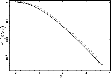
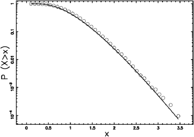
Figure 1 reports an example of SF in 2D PVT (areas) and Figure 2 an example of SF in 3D PVT (volumes).

Figure 1: SF of normalized area-distribution function in 2D when we have 25087 Poissonian seeds and $40$ intervals: the empty circles represent the Voronoi volumes and the full line the theoretical value of $S_{GG}$ (generalized gamma function) as represented by (13).

Figure 2: SF of normalized volume-distribution function in 3D when we have 21378 Poissonian seeds and $40$ intervals: the empty circles represent the Voronoi volumes and the full line the theoretical value of $S_{K}$ (Kiang function) as represented by (8).

3 Radius distribution of the 3D PVT

We now analyse the distribution in effective radius $R$ of the 3D PVT. We assume that the volume of each cell, $v$, is

$$v=\frac{4}{3}\pi(\frac{R}{\rho})^{3}\quad,$$ (24)

where $\rho$ is a length that connects the normalized radius to the observed one. In the following, we derive the PDF for radius and related quantities relative to the Kiang function and Ferenc–Neda function.

3.1 Kiang function of the radius

The PDF, $H_{R}(R;c)$, of the radius corresponding to the Kiang function as represented by (3) is

$$H_{R}(R;c)=\frac{4\,c\left(4/3\,{\frac{c\pi\,{R}^{3}}{{\rho}^{3}}}\right)^{c-1}{e^{-4/3\,{\frac{c\pi\,{R}^{3}}{{\rho}^{3}}}}}\pi\,{R}^{2}}{\Gamma\left(c\right){\rho}^{3}}\quad,$$ (25)

where $0\leq R<\infty$, $c~{}>0$ and $\rho~{}>0$. The Kiang PDF of the radius has a mean of

$$\mu=1/2\,{\frac{\sqrt[3]{2}\sqrt[3]{3}\Gamma\left(1/3+c\right)}{\sqrt[3]{c}\sqrt[3]{\pi}\Gamma\left(c\right)}}\rho\quad,$$ (26)

and variance

$$\sigma^{2}=$$

$$\frac{1}{4}{\frac{{3}^{\frac{2}{3}}{2}^{\frac{2}{3}}\left(\Gamma\left(2/3+c\right)\Gamma\left(c\right)-\left(\Gamma\left(1/3+c\right)\right)^{2}\right)}{{c}^{2/3}{\pi}^{2/3}\left(\Gamma\left(c\right)\right)^{2}}}\rho^{2}\quad.$$ (27)

The DF of the Kiang function of the radius is

$$DF_{KR}=1-{\frac{\Gamma\left(c,4/3\,c\pi\,(\frac{R}{\rho})^{3}\right)}{\Gamma\left(c\right)}}\quad.$$ (28)

The survival function of the radius is

$$S_{KR}={\frac{\Gamma\left(c,4/3\,c\pi\,(\frac{R}{\rho})^{3}\right)}{\Gamma\left(c\right)}}\quad.$$ (29)

3.2 The Ferenc–Neda function of the radius

The PDF as a function of the radius, obtained from (14) and inserting $d=3$, is

$$FN_{R}(R;d)=\frac{400000\,{\pi}^{5}{R}^{14}{e^{-{\frac{20}{3}}\,{\frac{\pi\,{R}^{3}}{{\rho}^{3}}}}}}{243\,{\rho}^{15}}\quad.$$ (30)

The mean of the Ferenc–Neda function is

$$\mu=0.6\rho\quad,$$ (31)

and the variance is

$$\sigma^{2}=0.0085\rho^{2}\quad.$$ (32)

The DF of the Ferenc–Neda function of the radius when $d=3$ is

$$DF_{FN3R}=$$

$$1-{e^{-{\frac{20}{3}}\,{\frac{\pi\,{R}^{3}}{{\rho}^{3}}}}}-{\frac{20}{3}}\,{e^{-{\frac{20}{3}}\,{\frac{\pi\,{R}^{3}}{{\rho}^{3}}}}}{R}^{3}\pi{\rho}^{-3}$$

$$-{\frac{200}{9}}\,{e^{-{\frac{20}{3}}\,{\frac{\pi\,{R}^{3}}{{\rho}^{3}}}}}{R}^{6}{\pi}^{2}{\rho}^{-6}$$

$$-{\frac{4000}{81}}\,{e^{-{\frac{20}{3}}\,{\frac{\pi\,{R}^{3}}{{\rho}^{3}}}}}{R}^{9}{\pi}^{3}{\rho}^{-9}$$

$$-{\frac{20000}{243}}\,{e^{-{\frac{20}{3}}\,{\frac{\pi\,{R}^{3}}{{\rho}^{3}}}}}{R}^{12}{\pi}^{4}{\rho}^{-12}\quad.$$ (33)

The SF of the Ferenc–Neda function of the radius when $d=3$ is

$$S_{FN3R}=$$

$${e^{-{\frac{20}{3}}\,{\frac{\pi\,{R}^{3}}{{\rho}^{3}}}}}+{\frac{20}{3}}\,{e^{-{\frac{20}{3}}\,{\frac{\pi\,{R}^{3}}{{\rho}^{3}}}}}{R}^{3}\pi{\rho}^{-3}$$

$$+{\frac{200}{9}}\,{e^{-{\frac{20}{3}}\,{\frac{\pi\,{R}^{3}}{{\rho}^{3}}}}}{R}^{6}{\pi}^{2}{\rho}^{-6}$$

$$+{\frac{4000}{81}}\,{e^{-{\frac{20}{3}}\,{\frac{\pi\,{R}^{3}}{{\rho}^{3}}}}}{R}^{9}{\pi}^{3}{\rho}^{-9}$$

$$+{\frac{20000}{243}}\,{e^{-{\frac{20}{3}}\,{\frac{\pi\,{R}^{3}}{{\rho}^{3}}}}}{R}^{12}{\pi}^{4}{\rho}^{-12}\quad.$$ (34)

4 Self-similar void distribution

The statistics of the voids between galaxies have been analysed in von Benda-Beckmann & Müller (2008) with the following self-similar SF in the following, $S_{SS}$,

$$S_{SS}={{\rm e}^{-\left({\frac{R}{s_{{1}}\lambda}}\right)^{p_{{1}}}-\left({\frac{R}{s_{{2}}\lambda}}\right)^{p_{{2}}}}}\quad,$$ (35)

where $\lambda$ is the mean separation between galaxies, $s_{1}$ and $s_{2}$ are two length factors, and $p_{1}$ and $p_{2}$ two powers. The DF of the self-similar distribution is

$$DF_{SS}=1-{{\rm e}^{-\left({\frac{R}{s_{{1}}\lambda}}\right)^{p_{{1}}}-\left({\frac{R}{s_{{2}}\lambda}}\right)^{p_{{2}}}}}\quad.$$ (36)

The PDF of the self-similar distribution is

$$p_{SS}(R)=$$

$$\frac{{{\rm e}^{-\left({\frac{R}{s_{{1}}\lambda}}\right)^{p_{{1}}}-\left({\frac{R}{s_{{2}}\lambda}}\right)^{p_{{2}}}}}\left(\left({\frac{R}{s_{{1}}\lambda}}\right)^{p_{{1}}}p_{{1}}+\left({\frac{R}{s_{{2}}\lambda}}\right)^{p_{{2}}}p_{{2}}\right)}{R}\quad.$$ (37)

At present, it is not possible to find an analytical expression for the integral that defines the average value of the self-similar distribution.

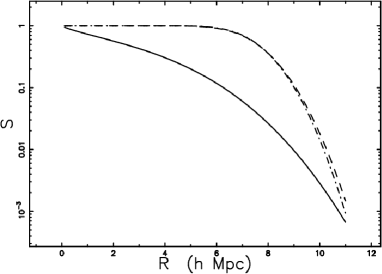
A comparison of the survival function of self-similar voids with the survival function of the radii of the two PDFs analysed here is reported in Figure 3.

Figure 3: The survival function, $S_{SS}$, of the self-similar distribution in radius of $N/S1$ as represented by (35) (full line), the survival function, $S_{FN3R}$, for the Ferenc–Neda function of the radius as represented by (34) when $d=3$, $\rho=12.5$ Mpc and $\chi^{2}=4319$ with 100 points (dashed line). The survival function, $S_{KR}$, of the radius of the Kiang function as represented by (29) when $\rho=12.5$ Mpc, $c=5.53$ and $\chi^{2}=4076$ with 100 points (dot-dash-dot-dash line).

The two fits of Figure 3 are not satisfactory because we are making a comparison between the radius of projected voids and the 3D radii of the normalized volume distribution of the PVT. This fact is confirmed from the high values of $\chi^{2}$ computed according to (23).

5 The sectional PVT

The existence of voids between galaxies is normally deduced from a projected distribution in astronomical slices such as the 2dFGRS S3, see Figure 1 in von Benda-Beckmann & Müller (2008). This fact motivates the analysis of the sectional Voronoi tessellation, also known as $V_{p}(2,3)$, see Okabe et al. (1992). A previous analysis has shown that a cell belonging to the intersection between an arbitrary plane and the faces of the Voronoi polyhedrons is almost surely a non-Voronoi cell, see details in Chiu et al. (1996). Here, we first model the normalized area-distribution $V_{p}(2,3)$ with Kiang PDFs as represented by (3), see Table 3.

Table 3: Values of $\chi^{2}$ for the cell normalized area-distribution function of $V_{p}(2,3)$; here $T_{i}$ are the theoretical frequencies and $O_{i}$ are the sample frequencies. Here we have 8517 Poissonian seeds and 40 intervals in the histogram.

$$\begin{array}[]{llll}\hline\cr PDF{}&parameters&\chi^{2}\\ \vskip 3.0pt plus 1.0pt minus 1.0pt\cr\hline\cr\vskip 3.0pt plus 1.0pt minus 1.0pt\cr H(x;c)~{}(Eq.(\ref{kiang}))&c=2.07&114.41\\ p(x;b)~{}(Eq.(\ref{exponential}))&d=1&85.38\\ \vskip 3.0pt plus 1.0pt minus 1.0pt\cr\hline\cr\hline\cr\end{array}$$

In the case of $n$ cuts, we can compute the average value of $c$, $\overline{c}$, and the standard deviation $\sigma$, see Table 4.

Table 4: Average value of $c$ according to the Kiang function, Eq. (3)), for $V_{p}(2,3)$, when 50 cuts are considered. Here we have 25087 Poissonian seeds.

$$\begin{array}[]{llll}\hline\cr PDF{}&name&\overline{c}&\sigma\\ \vskip 3.0pt plus 1.0pt minus 1.0pt\cr\hline\cr\vskip 3.0pt plus 1.0pt minus 1.0pt\cr H(x;c)~{}(Eq.(\ref{kiang}))&Kiang&2.25&0.11\\ \vskip 3.0pt plus 1.0pt minus 1.0pt\cr\hline\cr\hline\cr\end{array}$$

A test of this value can be done on the unpublished manuscript of Ken Brakke available at http://www.susqu.edu/brakke/aux/
downloads/papers/3d.pdf .
Table 4 of this paper is dedicated to the 3D plane cross-sectional statistics E(area) = 0.6858 and Var(area) = 0.2269. When a typical run of ours is normalized to the average value rather than 1, our result is Var(area) = 0.2266 which means that our numerical evaluation differs by 2/10000 from the theoretical result. We remember that in the case of the normalized area-distribution function in 2D we have $c\approx 4$ and we can therefore speak of a decrease in the value of $c$ by a factor 2. The decrease of $c$ for $V_{p}(2,3)$ was first derived in Figure 4 of Zaninetti (2006).

Another PDF that can be considered in order to model the normalized area distribution of $V_{p}(2,3)$ is the exponential distribution,

$$p(x)=\frac{1}{b}\exp{-\frac{x}{b}}\quad,$$ (38)

which has an average value

$$\overline{x}=b\quad.$$ (39)

In the case of the normalized areas $b=1$, Table 3 reports the $\chi^{2}$ values of the two distributions adopted here. Once the statistics of the normalized area distribution of an arbitrary cut $V_{p}(2,3)$ are known, we can model the radius distribution. We therefore convert the area of each cell, $A$, to an equivalent radius $R$

$$R=\sqrt{\frac{A}{\pi}}\quad.$$ (40)

We also briefly remember that the problem of stereology is to deduce the true size distribution $N(R)$ of 3D-volumes from the distribution $n(r)$ of apparent circles in 2D.

5.1 Kiang distribution of $V_{p}(2,3)$ in radius

The PDF, $H_{R23}(R;c)$, as a function of the radius corresponding to the Kiang function as represented by (3) for $V_{p}(2,3)$ is

$$H_{R23}(R;c)=\frac{2\,c\left({\frac{c\pi\,{R}^{2}}{{\rho}^{2}}}\right)^{c-1}{{\rm e}^{-{\frac{c\pi\,{R}^{2}}{{\rho}^{2}}}}}\pi\,R}{\Gamma\left(c\right){\rho}^{2}}\quad,$$ (41)

where $0\leq R<\infty$, $c~{}>0$ and $\rho~{}>0$. The Kiang PDF of the radius for $V_{p}(2,3)$ has a mean of

$$\mu={\frac{\rho\,\Gamma\left(c+1/2\right)}{\sqrt{c}\sqrt{\pi}\Gamma\left(c\right)}}\quad,$$ (42)

and variance

$$\sigma^{2}=\frac{{\rho}^{2}\left(c\left(\Gamma\left(c\right)\right)^{2}-\left(\Gamma\left(c+1/2\right)\right)^{2}\right)}{c\pi\,\left(\Gamma\left(c\right)\right)^{2}}\quad.$$ (43)

The DF of the Kiang function of the radius, $DF_{KR23}$, for $V_{p}(2,3)$ is:

$$DF_{KR23}=1-\frac{\Gamma\left(c,2\,{\frac{c\pi\,{R}^{2}}{{\rho}^{2}}}\right)}{\Gamma\left(c\right)}\quad.$$ (44)

The survival function $S_{KR23}$ of the radius for $V_{p}(2,3)$ is

$$S_{KR23}=\frac{\Gamma\left(c,2\,{\frac{c\pi\,{R}^{2}}{{\rho}^{2}}}\right)}{\Gamma\left(c\right)}\quad.$$ (45)

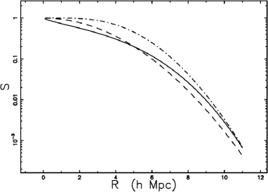
A comparison of the survival function of self-similar voids with the survival function of the radius for $V_{p}(2,3)$ of the exponential distribution is reported in Figure 4.

Figure 4: The survival function, $S_{SS}$, of the self-similar distribution in radius of $N/S1$ as represented by (35) (full line), the survival function, $S_{KR23}$, of the radius of the Kiang function for $V_{p}(2,3)$ as represented by (45) when $\rho=13$ Mpc, $c=2.25$ and $\chi^{2}=67.1$ with 100 points (dot-dash-dot-dash line). The survival function, $S_{ER23}$, of the radius of the exponential distribution for $V_{p}(2,3)$ as represented by (50) when $\rho=7$ Mpc and $\chi^{2}=9.27$ with 100 points (dashed line).

5.2 Exponential distribution of $V_{p}(2,3)$ in radius

The PDF, $p_{R23}(R;c)$, as a function of the radius corresponding to the exponential distribution as represented by (38) for $V_{p}(2,3)$ is

$$p_{R23}(R;c)=\frac{2\,{{\rm e}^{-{\frac{\pi\,{R}^{2}}{{\rho}^{2}}}}}\pi\,R}{{\rho}^{2}}\quad,$$ (46)

where $0\leq R<\infty$, $\rho>0$. The exponential PDF of the radius for $V_{p}(2,3)$ has a mean of

$$\mu=\frac{{\pi}^{3/2}}{2\,{\rho}^{2}\left({\frac{\pi}{{\rho}^{2}}}\right)^{3/2}}\quad,$$ (47)

and variance

$$\sigma^{2}=\frac{{\rho}^{2}\left(4-\pi\right)}{4\,\pi}\quad.$$ (48)

The DF of the exponential distribution in radius, $DF_{ER23}$, for $V_{p}(2,3)$ is:

$$DF_{ER23}=1-{{\rm e}^{-{\frac{\pi\,{R}^{2}}{{\rho}^{2}}}}}\quad.$$ (49)

The survival function $S_{ER23}$ of the radius for $V_{p}(2,3)$ is

$$S_{ER23}={{\rm e}^{-{\frac{\pi\,{R}^{2}}{{\rho}^{2}}}}}\quad.$$ (50)

Figure 4 reports a comparison between the survival function of self-similar voids and the exponential distribution for $V_{p}(2,3)$.

In this case, the two types of fit of Figure  4 are satisfactory because we are making a comparison between the observed projected radius of voids and the projected radius of the Voronoi volumes. The smaller $\chi^{2}$ associated with the exponential distribution can be considered a consequence of the fact that the statistics of the normalized area distribution of the cuts are better described by an exponential distribution than by the Kiang function, see Table 3.

A final comparison between the four samples of void size statistics as represented in Figure 4 of von Benda-Beckmann & Müller (2008) and our survival function of the radius of the exponential distribution for $V_{p}(2,3)$ is reported in Figure 5.

Figure 5: The survival function, $S_{SS}$, for the self-similar distribution in radius of $N/S1$, $N/S2$, $N/S3$ and $N/S4$, as reported in Figure 4 of von Benda-Beckmann and Muller 2008 (full red lines), as represented by (35). The survival function, $S_{ER23}$, of the radius of the exponential distribution for $V_{p}(2,3)$ as represented by (50) when $\rho=7$ Mpc, $\rho=9$ Mpc, $\rho=13$ Mpc and $\rho=17.7$ Mpc (dashed green lines).

6 Large-scale structure

We briefly review the status of the knowledge of the Hubble constant, reference magnitude of the sun, luminosity function of galaxies, Malmquist bias and 3D Poissonian Voronoi diagrams.

6.1 The adopted constants

A first important evaluation of the Hubble constant is through Cepheids (key programs with HST) and type Ia Supernovae, see Sandage et al. (2006), $H_{0}=(62.3\pm 5)\mathrm{\ km\ s}^{-1}\mathrm{\ Mpc}^{-1}$. A second important evaluation comes from three years of observations with the Wilkinson Microwave Anisotropy Probe, see Table 2 in Spergel et al. (2007), $H_{0}=(73.2\pm 3.2)\mathrm{\ km\ s}^{-1}\mathrm{\ Mpc}^{-1}$. In the following, we will take the average value of these two important evaluations, $H_{0}=67.65\mathrm{\ km\ s}^{-1}\mathrm{\ Mpc}^{-1}$. The Hubble constant is also reported as
$H_{0}=100h\mathrm{\ km\ s}^{-1}\mathrm{\ Mpc}^{-1}$, with $h=1$ when $h$ is not specified; in our case $h=.6765$.

Another quantity that should be fixed in order to continue is the absolute magnitude of the sun in the b_J filter of the 2dFGRS $\mathcal{M_{\hbox{$\odot$}}}$ = 5.33, see Colless et al. (2001); Tempel et al. (2009); Eke et al. (2004).

6.2 Malmquist bias

This bias was originally applied to the stars, see Malmquist (1920, 1922), and was then applied to the galaxies by Behr (1951). We now introduce the concept of limiting apparent magnitude and the corresponding completeness in absolute magnitude of the considered catalog as a function of redshift. The observable absolute magnitude as a function of the limiting apparent magnitude, $m_{L}$, is

$$M_{L}=m_{{L}}-5\,{\it\log_{10}}\left({\frac{{\it c}\,z}{H_{{0}}}}\right)-25\quad.$$ (51)

The previous formula predicts, from a theoretical point of view, an upper limit on the absolute maximum magnitude that can be observed in a catalog of galaxies characterized by a given limiting magnitude.

The interval covered by the LF of galaxies, $\Delta M$, is defined by

$$\Delta M=M_{max}-M_{min}\quad,$$ (52)

where $M_{max}$ and $M_{min}$ are the maximum and minimum absolute magnitude of the LF for the considered catalog. The real observable interval in absolute magnitude, $\Delta M_{L}$, is

$$\Delta M_{L}=M_{L}-M_{min}\quad.$$ (53)

We can therefore introduce the range of observable absolute maximum magnitude expressed in percent, $\epsilon(z)$, as

$$\epsilon_{s}(z)=\frac{\Delta M_{L}}{\Delta M}\times 100\,\%\quad.$$ (54)

This is a number that represents the completeness of the sample and, given the fact that the limiting magnitude of the 2dFGRS is $m_{L}$=19.61, it is possible to conclude that the 2dFGRS is complete for $z\leq 0.0442$ . This efficiency, expressed as a percentage, can be considered to be a version of the Malmquist bias.

6.3 Luminosity function of galaxies

The Schechter function, introduced by Schechter (1976), provides a useful fit for the LF (luminosity function) of galaxies

$$\Phi(L)dL=(\frac{\Phi^{*}}{L^{*}})(\frac{L}{L^{*}})^{\alpha}\exp\bigl{(}{-\frac{L}{L^{*}}}\bigr{)}dL\quad.$$ (55)

Here, $\alpha$ sets the slope for low values of $L$, $L^{*}$ is the characteristic luminosity and $\Phi^{*}$ is the normalization. The equivalent distribution in absolute magnitude is

$$\Phi(M)dM= (0.4ln10)\Phi^{*}10^{0.4(\alpha+1)(M^{*}-M)}$$ (56)

$$\times\exp\bigl{(}{-10^{0.4(M^{*}-M)}}\bigr{)}dM\quad,$$

where $M^{*}$ is the characteristic magnitude as derived from the data. The parameters of the Schechter function for the 2dFGRS can be found on the first line of Table 3 in Madgwick et al. (2002) and are reported in Table 5.

Table 5: Parameters of the Schechter function for
the 2dFGRS.

$$\begin{array}[]{lc}\hline\cr\hline\cr\vskip 3.0pt plus 1.0pt minus 1.0pt\cr parameter&2dFGRS\\ \vskip 3.0pt plus 1.0pt minus 1.0pt\cr M^{*}-5\log_{10}h~{}[mags]&(-19.79\pm 0.04)\\ \vskip 3.0pt plus 1.0pt minus 1.0pt\cr\alpha&-1.19\pm 0.01\\ \vskip 3.0pt plus 1.0pt minus 1.0pt\cr\Phi^{*}~{}[h^{3}~{}Mpc^{-3}]&((1.59\pm 0.1)10^{-2})\\ \vskip 3.0pt plus 1.0pt minus 1.0pt\cr\hline\cr\hline\cr\end{array}$$

We now introduce $f$, the flux of radiation expressed in units of $L_{\hbox{$\odot$}}$ Mpc^-2, with $L_{\hbox{$\odot$}}$ representing the luminosity of the sun. The joint distribution in z, redshift and f, see (1.104) in Padmanabhan (1996) or (1.117) in Padmanabhan (2002), is

$$\frac{dN}{d\Omega dzdf}=4\pi\bigl{(}\frac{c_{l}}{H_{0}}\bigr{)}^{5}z^{4}\Phi(\frac{z^{2}}{z_{crit}^{2}})\quad,$$ (57)

where $d\Omega$, $dz$, and $df$ represent the differential of the solid angle, redshift, flux and $c_{l}$ represents the velocity of light.

This relationship has been derived assuming $z\approx\frac{V}{c_{l}}\approx\frac{H_{0}r}{c_{l}}$ with $r$ representing the distance of the galaxy in Mpc. The critical value of $z$, $z_{crit}$, is

$$z_{crit}^{2}=\frac{H_{0}^{2}L^{*}}{4\pi fc_{l}^{2}}\quad.$$ (58)

The number of galaxies in $z$ and $f$ as given by (57) has a maximum at $z=z_{pos-max}$, where

$$z_{pos-max}=z_{crit}\sqrt{\alpha+2}\quad,$$ (59)

which can be re-expressed as

$$z_{pos-max}=\frac{\sqrt{2+\alpha}\sqrt{{10}^{0.4\,{\it M_{\hbox{$\odot$}}}-0.4\,{\it M^{*}}}}{\it H_{0}}}{2\,\sqrt{\pi}\sqrt{f}{\it c_{l}}}\quad.$$ (60)

The number of galaxies, $N_{S}(z,f_{min},f_{max})$, comprised between the minimum value of flux, $f_{min}$, and the maximum value of flux, $f_{max}$, can be computed with the following integral

$$N_{S}(z)=\int_{f_{min}}^{f_{max}}4\pi\bigl{(}\frac{c_{l}}{H_{0}}\bigr{)}^{5}z^{4}\Phi(\frac{z^{2}}{z_{crit}^{2}})df\quad.$$ (61)

This integral does not have an analytical solution and therefore a numerical integration must be performed. The total number of galaxies in the 2dFGRS is reported in Figure 6 as well as the theoretical curves as represented by the numerical integration of (57).

Figure 6: The galaxies in the 2dFGRS with $13.34\leq bJmag\leq 19.61$ or 1540 $L_{\hbox{$\odot$}}$ Mpc${}^{-2}\leq f\leq 493844L_{\hbox{$\odot$}}$ Mpc^-2, are organized as frequencies versus heliocentric redshift (empty stars). The theoretical curve generated by the integral of the Schechter function in flux, (61, (full line) is drawn. The maximum in the frequencies of observed galaxies is at $z=0.108$. In this plot, $\mathcal{M_{\hbox{$\odot$}}}$ = 5.33 and $h$ = 0.67. The vertical dotted line represents the boundary between complete and incomplete samples.

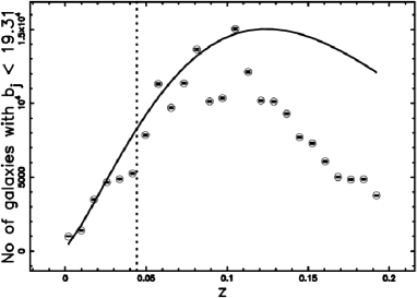
A careful inspection of the previous figure allows to conclude that the theoretical integral fits well the experimental data up to $z=0.0442$. Beyond that value, the presence of the Malmquist bias decreases the number of observable galaxies and the comparison between theory and observations cannot be made.

6.4 Voronoi diagrams

Voronoi diagrams represent a useful tool for describing the spatial distribution of galaxies and, as an example, van de Weygaert & Icke (1989) identified the vertexes of irregular Voronoi polyhedrons with Abell clusters. Another example is provided by Zaninetti (1991) where the galaxies were first inserted on the faces of the irregular Voronoi polyhedrons and a power law distribution for the seeds was adopted. Later, the galaxies were still inserted on the faces of the irregular Voronoi polyhedrons but Poissonian seeds were adopted, see Zaninetti (2006, 2008, 2010). Adopting the same algorithm developed in Zaninetti (2010), one slice of the 2dFGRS with the number of galaxies as a function of $z$ as given by (61) is simulated, see Figure 7.

Figure 7: A Voronoi slice $75^{\circ}$ long and $3^{\circ}$ wide. The range of the flux is 2500 $L_{\hbox{$\odot$}}$ Mpc${}^{-2}\leq f\leq 286808L_{\hbox{$\odot$}}$ Mpc^-2 and the number of galaxies is 19895. The red circle denotes the confusion distance as given by (64).

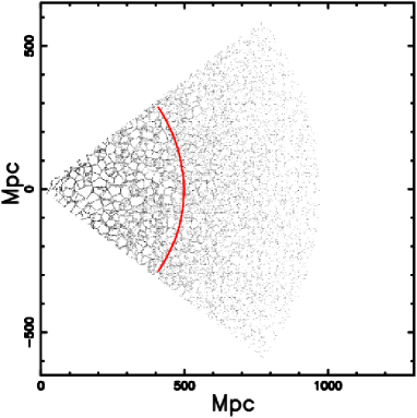
This simulation should be compared with Figure 1 in von Benda-Beckmann & Müller (2008) and with a $3^{\circ}$ slice of the 2dFGRS Image Gallery available at the web site, http://msowww.anu.edu.au/2dFGRS/. Little need be said about the number of seeds which should be used in order to simulate the observed slices of the 2dFGRS. The average volume of the voids is the side of the box in Mpc divided by the number of seeds. The average diameter of the voids, $D_{Voronoi}$, is

$$D_{Voronoi}=(\frac{side[Mpc]}{No~{}of~{}seeds})^{1/3}\quad.$$ (62)

The theoretical average diameter, $D_{th}$, can be obtained from the average value (47 ) of the exponential distribution of $V_{p}(2,3)$ in radius once the maximum value of $\rho$ which fits the von Benda-Beckmann & Müller (2008) data, see Figure 5, is adopted

$$D_{th}=\mu\frac{2}{h}\quad.$$ (63)

The equality $D_{Voronoi}=D_{th}$ allows to obtain the number of Poissonian seeds.

Particular attention should be paid to the fact that the astronomical slices are not a plane which intersects a Voronoi network. In order to quantify this effect, we introduce a confusion distance, $D_{c}$, as the distance after which the altitude of the slices equalizes the observed average diameter $\overline{D_{obs}}$

$$D_{c}\tan(\alpha)=\overline{D_{obs}}\quad,$$ (64)

where $\alpha$ is the opening angle of the slice and $\overline{D_{obs}}$ is the average diameter of the voids. In the case of 2dFGRS $\alpha=3^{\circ}$ and therefore $D_{c}=498.5$ Mpc when $D_{obs}=26.12$ Mpc, see the red circle in Figure 7.

7 Conclusions

The PDFs which are usually used to model the normalized volume distribution of the 3D PVT are gamma type distributions such as the Kiang function, (3), and the new Ferenc–Neda function, (14).

Here, in order to make a comparison with the self-similar distribution of voids, we derived the survival distribution of the Kiang function, (8), and of the Ferenc–Neda function, (22).

On adopting an astrophysical point of view the cut $V_{p}(2,3)$ may model the voids between galaxies as given by astronomical slices of the Millenium catalog. The analysis of the normalized areas of $V_{p}(2,3)$ is a subject of research rather than a well-established fact and we have fitted them with the Kiang function and the exponential distribution. The $\chi^{2}$ value indicates that the exponential distribution fits more closely the normalized area distribution of $V_{p}(2,3)$ than does the Kiang function, see Table 3. This fact follows from the comparison between the self-similar survival function and the exponential and Kiang distributions of the radius, see Figure 4. Therefore, the one parameter survival function of the radius of the exponential distribution for $V_{p}(2,3)$, $S_{ER23}$, as represented by (50), may model the voids between galaxies as well as the five parameter self-similar survival function.

The observed 2dFGRS slices can be simulated but the behaviour of the luminosity function for galaxies and the consequent number of galaxies as a function of the redshift should be carefully analysed.

We are planning, in future projects,

• To insert the thickness of the faces of PVT and to model the connected modification of the survival function.

• To apply the technique here developed to the real data sets, Millennium simulation, for example. The 3D nature of the method and detailed density mapping of the voids should be superior to other void identification algorithms as suggested by van de Weygaert & Schaap (2009).

References

- Aurenhammer, F. and Klein, R. In : Sack, J.-R. (2000) Aurenhammer, F. and Klein, R. In : Sack, J.-R., ed. 2000, Voronoi diagrams. (Amsterdam: North-Holland)
- Barrow & Coles (1990) Barrow, J. D. & Coles, P. : 1990, MNRAS , 244, 188
- Behr (1951) Behr, A. : 1951, Astronomische Nachrichten, 279, 97
- Bernardeau & van de Weygaert (1996) Bernardeau, F. & van de Weygaert, R. : 1996, MNRAS , 279, 693
- Chiu et al. (1996) Chiu, S. N., Weygaert, R. V. D., & Stoyan, D. : 1996, Advances in Applied Probability, 28, 356
- Coles (1991) Coles, P. : 1991, Nature , 349, 288
- Colless et al. (2001) Colless, M., Dalton, G., Maddox, S., & et al. : 2001, MNRAS , 328, 1039
- Descartes (1644) Descartes, R. : 1644, Principia Philosophiae (Amsterdam: Ludovicus Elzevirius)
- Ebeling & Wiedenmann (1993) Ebeling, H. & Wiedenmann, G. : 1993, Phys. Rev. E , 47, 704
- Einasto et al. (2003) Einasto, J., Hütsi, G., Einasto, M., et al. : 2003, A&A , 405, 425
- Eke et al. (2004) Eke, V. R., Frenk, C. S., Baugh, C. M., Cole, S., & Norberg, P. : 2004, MNRAS , 355, 769
- Elyiv et al. (2009) Elyiv, A., Melnyk, O., & Vavilova, I. : 2009, MNRAS , 394, 1409
- Ferenc & Néda (2007) Ferenc, J.-S. & Néda, Z. : 2007, Phys. A , 385, 518
- Geller & Huchra (1989) Geller, M. J. & Huchra, J. P. : 1989, Science, 246, 897
- Goldwirth et al. (1995) Goldwirth, D. S., da Costa, L. N., & van de Weygaert, R. : 1995, MNRAS , 275, 1185
- Hinde & Miles (1980) Hinde , A. L. & Miles, R. : 1980, J. Stat. Comput. Simul., 10, 205
- Ikeuchi & Turner (1991) Ikeuchi, S. & Turner, E. L. : 1991, MNRAS , 250, 519
- Jones et al. (2004) Jones, D. H., Saunders, W., Colless, M., Read, M. A., & Parker, Q. A. e. : 2004, MNRAS , 355, 747
- Kiang (1966) Kiang, T. : 1966, Z. Astrophys. , 64, 433
- Madgwick et al. (2002) Madgwick, D. S., Lahav, O., Baldry, I. K., et al. : 2002, MNRAS , 333, 133
- Malmquist (1920) Malmquist , K. : 1920, Lund Medd. Ser. II, 22, 1
- Malmquist (1922) Malmquist , K. : 1922, Lund Medd. Ser. I, 100, 1
- Marinoni et al. (2002) Marinoni, C., Davis, M., Newman, J. A., & Coil, A. L. : 2002, ApJ , 580, 122
- Melnyk et al. (2006) Melnyk, O. V., Elyiv, A. A., & Vavilova, I. B. : 2006, Kinematika i Fizika Nebesnykh Tel, 22, 283
- Norberg et al. (2002) Norberg, P., Baugh, C. M., Hawkins, E., Maddox, S., & Madgwick, D. e. a. : 2002, MNRAS , 332, 827
- Okabe et al. (1992) Okabe, A., Boots, B., & Sugihara, K. : 1992, Spatial Tessellations. Concepts and Applications of Voronoi diagrams (Chichester, NY: Wiley)
- Padmanabhan (2002) Padmanabhan, P. : 2002, Theoretical Astrophysics. Vol. III: Galaxies and Cosmology (Cambridge: Cambridge University Press)
- Padmanabhan (1996) Padmanabhan, T. : 1996, Cosmology and Astrophysics through Problems (Cambridge: Cambridge University Press)
- Patiri et al. (2006) Patiri, S. G., Betancort-Rijo, J. E., Prada, F., Klypin, A., & Gottlöber, S. : 2006, MNRAS , 369, 335
- Pierre (1990) Pierre, M. : 1990, A&A , 229, 7
- Press et al. (1992) Press, W. H., Teukolsky, S. A., Vetterling, W. T., & Flannery, B. P. : 1992, Numerical Recipes in FORTRAN. The Art of Scientific Computing (Cambridge: Cambridge University Press)
- Sandage et al. (2006) Sandage, A., Tammann, G. A., Saha, A., et al. : 2006, ApJ , 653, 843
- Schaap & van de Weygaert (2000) Schaap, W. E. & van de Weygaert, R. : 2000, A&A , 363, L29
- Schechter (1976) Schechter, P. : 1976, ApJ , 203, 297
- Spergel et al. (2007) Spergel, D. N., Bean, R., Doré, O., Nolta, M. R., & Bennett, C. L. e. a. : 2007, ApJS , 170, 377
- Subba Rao & Szalay (1992) Subba Rao, M. U. & Szalay, A. S. : 1992, ApJ , 391, 483
- Tanemura (2003) Tanemura, M. : 2003, Forma, 18, 221
- Tempel et al. (2009) Tempel, E., Einasto, J., Einasto, M., Saar, E., & Tago, E. : 2009, A&A , 495, 37
- Tikhonov (2007) Tikhonov, A. V. : 2007, Astronomy Letters, 33, 499
- Tinker et al. (2008) Tinker, J. L., Conroy, C., Norberg, P., et al. : 2008, ApJ , 686, 53
- van de Weygaert (1991) van de Weygaert , R. : 1991, MNRAS , 249, 159
- van de Weygaert (1991) van de Weygaert, R. : 1991, Ph.D. thesis, University of Leiden
- van de Weygaert (1994) van de Weygaert, R. : 1994, A&A , 283, 361
- van de Weygaert (2002) van de Weygaert, R. : 2002, arXiv:astro-ph/0206427
- van de Weygaert (2003) van de Weygaert, R. 2003, Statistics of Galaxy Clustering - Commentary (Statistical Challenges in Astronomy), 156–186
- van de Weygaert & Icke (1989) van de Weygaert, R. & Icke, V. : 1989, A&A , 213, 1
- van de Weygaert & Schaap (2009) van de Weygaert, R. & Schaap, W. 2009, in Lecture Notes in Physics, Berlin Springer Verlag, Vol. 665, Lecture Notes in Physics, Berlin Springer Verlag, ed. V. J. Martinez, E. Saar, E. M. Gonzales, & M. J. Pons-Borderia , 291–+
- von Benda-Beckmann & Müller (2008) von Benda-Beckmann, A. M. & Müller, V. : 2008, MNRAS , 384, 1189
- Voronoi (1907) Voronoi, G. : 1907, J. Reine Angew. Math, 133, 97
- Voronoi (1908) Voronoi, G. : 1908, J. Reine Angew. Math, 134, 198
- Zaninetti (1991) Zaninetti, L. : 1991, A&A , 246, 291
- Zaninetti (2006) Zaninetti, L. : 2006, Chinese J. Astron. Astrophys. , 6, 387
- Zaninetti (2008) Zaninetti, L. : 2008, Acta Physica Polonica B, 39, 1467
- Zaninetti (2010) Zaninetti, L. : 2010, Revista Mexicana de Astronomia y Astrofisica, 46, 115