Iterative Beam Search for Simple Assembly Line Balancing with a Fixed Number of Work Stations

Abstract

The simple assembly line balancing problem (SALBP) concerns the assignment of tasks with pre-defined processing times to work stations that are arranged in a line. Hereby, precedence constraints between the tasks must be respected. The optimization goal of the SALBP-2 version of the problem concerns the minimization of the so-called cycle time, that is, the time in which the tasks of each work station must be completed.

In this work we propose to tackle this problem with an iterative search method based on beam search. The proposed algorithm is able to obtain optimal, respectively best-known, solutions in 283 out of 302 test cases. Moreover, for 9 further test cases the algorithm is able to produce new best-known solutions. These numbers indicate that the proposed iterative beam search algorithm is currently a state-of-the-art method for the SALBP-2.

1 Introduction

The class of problems known as assembly line balancing problems (ALBPs) concerns the optimization of processes related to the manufacturing of products via assembly lines. Their importance in the industrial world is shown by the fact that much research efforts have been dedicated to many different types of ALBPs during the past 50-60 years [18, 8]. The specific problem considered in this paper is the so-called simple assembly line balancing problem (SALBP) [21], a well-studied scientific test case. An assembly line is composed of a set of work stations arranged in a line, and by a transport system which moves the product to be manufactured along the line. The product is manufactured by executing a given set of tasks. Each of these tasks has a pre-defined processing time. In order to obtain a solution to a given SALBP instance, all tasks must be assigned to work stations subject to precedence constraints between the tasks. In the context of the SALBP, all work stations are considered to be of equal size. Moreover, the assembly line is assumed to move in constant speed. This implies a maximum of $C$ time units—the so-called cycle time—for processing the tasks assigned to each work station. The SALBP has been tackled with several objective functions among which the following ones are the most studied ones in the literature:

• Given a fixed cycle time $C$, the optimization goal consists in minimizing the number of necessary work stations. This version of the problem is refered to as SALBP-1.

• Given a fixed number $m$ of work stations, the goal is to minimize the cycle time $C$. The literature knows this second problem version as SALBP-2.

The feasibility problem SALBP-F arises when both a cycle time $C$ and a number of work stations $m$ is given and the goal is to find a feasible solution respecting $C$ and $m$. In this work we will deal with the SALBP-2 version of the problem.

For what concerns the comparison between SALBP-1 and SALBP-2, much of the scientific work has been dedicated to the SALBP-1. However, also for the SALBP-2 exists a considerable body of research papers. An excellent survey was provided by [21]. Approaches for the SALBP-2 can basically be classified as either iterative solution approaches or direct solution approaches. Iterative approaches tackle the problem by iteratively solving a series of SALBP-F problems that are obtained by fixing the cycle time. This process is started with a cycle time that is set to some calculated upper bound. This cycle time is then decremented during the iterative process, which stops as soon as no solution for the corresponding SALBP-F problem can be found. In contrast to these indirect approaches, direct approaches intend to solve a given SALBP-2 instance directly.

Heuristic as well as complete approaches have been devised for the SALBP-2. Among the existing complete methods we find iterative approaches such as the ones proposed in [9, 20] but also direct approaches such as the ones described in [19, 12]. Moreover, the performance of different integer programming formulation of the SALBP-2 has been evaluated in [16]. The currently best-performing exact method is SALOME-2 [12]. Surprisingly this exact method even outperforms the existing heuristic and metaheuristic approaches for the SALBP-2. The most successful metaheuristic approach to date is a tabu search method proposed in [22]. Another tabu search proposal can be found in [6]. Other metaheuristic approaches include evolutionary algorithms [2, 25, 14] and simulated annealing [10]. Finally, a two-phase heuristic based on linear programming can be found in [23], whereas a heuristic based on Petri nets was proposed in [11].

Contribution of this work.

Subsequently we propose to tackle the SALBP-2 by means of an iterative approach based on beam search, which is an incomplete variant of branch & bound. The resulting iterative beam search algorithm is inspired by one of the current state-of-the-art methods for the SALBP-1, namely Beam-ACO [3]. Beam-ACO is a hybrid approach that is obtained by combining the metaheuristic ant colony optimization with beam search. In this work we propose to use the beam search component of Beam-ACO in an iterative way for obtaining good SALBP-2 solutions. Our computational results show indeed that the proposed algorithm is currently a state-of-the-art method for the SALBP-2. It is able to obtain optimal, respectively best-known, solutions in 283 out of 302 test cases. Moreover, in further 9 cases the algorithm is able to produce new best-known solutions.

Organization of the paper.

In Section 2 we present a technical description of the tackled problem. Furthermore, in Section 3 the proposed algorithm is described. Finally, in Section 4 we present a detailed experimental evaluation and in Section 5 we conclude our work and offer an outlook to future work.

2 The SALBP-2

The SALBP-2 can technically be described as follows. An instance $(T,G,m)$ consists of three components. $T=\{1,\ldots,n\}$ is a set of $n$ tasks. Each task $i\in T$ has a pre-defined processing time $t_{i}>0$. Moreover, given is a precedence graph $G=(T,A)$, which is a directed, acyclic graph with $T$ as node set. Finally, $m$ is the pre-defined number of work stations which are ordered from 1 to $m$. An arc $l_{i,j}\in A$ indicates that $i\in T$ must be processed before $j\in T$. Given a task $j\in T$, $P_{j}\subset T$ denotes the set of tasks that must be processed before $j$. A feasible solution is obtained by assigning each task to exactly one work station such that the precedence constraints between the tasks are satisfied. The objective function consists in minimizing the so-called cycle time. The SALBP-2 can be expressed in the following way as an integer programming (IP) problem.

$$\mbox{\bf min }z$$ (1)

subject to:

$$\sum\limits_{s=1}^{m}x_{is} = 1\;\;\;\forall i\in T$$ (2)

$$\sum\limits_{s=1}^{m}sx_{is} \leq \sum\limits_{s=1}^{m}sx_{js}\;\;\;\forall j\in T,i\in P_{j}$$ (3)

$$\sum\limits_{i\in T}t_{i}x_{is} \leq z\;\;\;s=1,\ldots,m$$ (4)

$$x_{is} \in \{0,1\}\;\;\;\forall i\in T,s=1,\ldots,m$$ (5)

$$z > 0$$ (6)

This IP model makes use of the following variables and constants: $x_{is}$ is a binary variable which is set to 1 if and only if task $i\in T$ is assigned to work station $1\leq s\leq m$. The objective function (1) minimizes the cycle time $z>0$. The constraints (2) ensure that each task $i\in T$ is assigned to a single work station $1\leq s\leq m$. Constraints (3) reflect the precedence relationships between the tasks. More specifically, if task $j\in T$ is assigned to a work station $1\leq s\leq m$, all tasks $i\in P_{j}$ must be assigned to work stations $1\leq s^{\prime}\leq m$ with $s^{\prime}\leq s$. The constraints (4) ensure that the sum of the processing times of the tasks assigned to a work station $1\leq s\leq m$ do not exceed the cycle time $z$. Note that this model is not necessarily the most efficient IP model for solving the SALBP-2. An evaluation of several different models can be found in [16].

2.1 Solution Representation

The following solution representation is used for the description of the algorithm as given in Section 3. A solution $\mathcal{S}$ is an ordered list $\mathcal{S}=\langle S_{1},\ldots,S_{m}\rangle$ of $m$ sets of tasks, where $S_{i}$ denotes the set of tasks that are assigned to the $i$-th work station. Abusing notation we henceforth call $S_{i}$ a work station. Note that for a solution $\mathcal{S}$ to be valid the following conditions must be fulfilled:

1. $\bigcup_{i=1}^{m}S_{i}=T=\{1,\ldots,n\}$ and $\bigcap_{i=1}^{m}S_{i}=\emptyset$, that is, each task is assigned to exactly one work station.

2. For each task $j\in S_{i}$ it is must hold that $P_{j}\subseteq\bigcup_{k=1}^{i}S_{k}$. This ensures that the precedence constraints between the tasks are not violated.

2.2 Reverse Problem Instances

The reverse problem instance $(T,G^{r},m)$ with respect to an original instance $(T,G,m)$ is obtained by inverting the direction of all arcs of $G$. It is well-known from the literature [21] that tackling the reverse problem instance may lead an exact algorithm faster to an optimal solution, respectively, may provide a better heuristic solution when tackled with the same heuristic as the original problem instance. Moreover, a solution $\mathcal{S}^{r}$ to the reverse problem instance $(T,G^{r},m)$ can easily be converted into a solution $\mathcal{S}$ to the original problem instance $(T,G,m)$ as follows:

$$S_{i}:=S^{r}_{m-i+1}\quad\mbox{for }i=1,\ldots,m$$ (7)

3 Iterative Beam Search

As mentioned in the introduction, the basic component of our algorithm for the SALBP-2 consists of beam search (BS), which is an incomplete derivative of branch & bound [15]. Initially BS has especially been used in the context of scheduling problems (see, for example, [17, 7, 24]). To date only very few applications to other types of problems exist (see, for example, [13, 1, 4]). In the following we briefly describe how one of the standard versions of BS works. The crucial aspect of BS is the parallel extension of partial solutions in several ways. At all times, the algorithm keeps a set $B$ of at most $k_{\text{\tiny bw}}$ partial solutions, where $B$ is the so-called beam, and $k_{\text{\tiny bw}}$ is known as the beam width. At each step, at most $k_{\mbox{\tiny ext}}$ feasible extensions of each partial solution in $B$ are selected on the basis of greedy information. In general, this selection is done deterministically. At the end of each step, the algorithm creates a new beam $B$ by choosing up to $k_{\text{\tiny bw}}$ partial solutions from the set of selected feasible extensions. For that purpose, BS algorithms determine—in the case of minimization—a lower bound value for each extension. Only the maximally $k_{\text{\tiny bw}}$ best extensions—with respect to these lower bound values—are included in $B$. Finally, if any complete solution was generated, the algorithm returns the best of those. Note that the underlying constructive heuristic that defines feasible extensions of partial solutions and the lower bound function for evaluating partial solutions are crucial for the working of BS.

In the following we first present a description of the implementation of the BS component, before we describe the algorithmic scheme in which this BS component is used.

3.1 The Beam Search Component

The BS component described in this section—see Algorithm 1 for the pseudo-code—is the main component of the proposed algorithm for the SALBP-2. The algorithm requires a problem instance $(T,G,m)$, a fixed cycle time $C$, a beam width $k_{\text{\tiny bw}}$, and a maximal number of extensions $k_{\mbox{\tiny ext}}$ as input. Given a fixed cycle time $C$ and $m$ (the number of work stations) BS tries to find at least one feasible solution. As mentioned before, the crucial aspect of BS is the extension of partial solutions in several possible ways. At each step the algorithm extends each partial solution from $B$ in a maximum number of ways. More specifically, given a partial solution with $l-1<m$ work stations already filled, an extension is generated by assigning a set of so-far unassigned tasks to the next work station $S_{l}$ such that the given cycle time $C$ is not surpassed and the precedence constraints between the tasks are respected (see lines 11–12 of Algorithm 1). The algorithm produces extensions in a (partially) probabilistic way rather than in the usual deterministic manner. Each generated extension (partial solution) is either stored in set $B_{\mbox{\tiny compl}}$ in case it is a complete solution, or in set $B_{\mbox{\tiny ext}}$ otherwise (see lines 13–19 of Algorithm 1). However, a partial solution is only stored in set $B_{\mbox{\tiny ext}}$ if it uses at most $m-1$ work stations, and if its $l$-th work station is different to the $l$-th work station of all partial solutions that are already in $B$. Finally, BS creates a new beam $B$ by selecting up to $k_{\mbox{\tiny bw}}$ solutions from set $B_{\mbox{\tiny ext}}$ of further extensible partial solutions (see line 22 of Algorithm 1). This is done in function SelectSolutions($B_{\mbox{\tiny ext}}$,$k_{\mbox{\tiny bw}}$) on the basis of a lower bound function LB$(\cdot)$. In the following we describe in detail the extension of partial solutions and the working of function SelectSolutions($B_{\mbox{\tiny ext}}$,$k_{\mbox{\tiny bw}}$).

Algorithm 1 Beam search

1:  input: an instance $(T,G,m)$, a fixed cycle time $C$, a beam width $k_{\text{\tiny bw}}$, and $k_{\mbox{\tiny ext}}$

2:  $l:=0$

3:  Initialization of an empty solution $\mathcal{S}$

4:  $B:=\{\mathcal{S}\}$

5:  $B_{\mbox{\tiny compl}}:=\emptyset$

6:  while $B\not=\emptyset$ do

7:     $B_{\mbox{\tiny ext}}:=\emptyset$

8:     $l:=l+1$

9:     for all $\mathcal{S}\in B$ do

10:        for $i=1,\ldots,k_{\mbox{\tiny ext}}$ do

11:           $\mathcal{S}^{\prime}:=\mathcal{S}$ {copy partial solution $\mathcal{S}$ into $\mathcal{S}^{\prime}$}

12:           $S^{\prime}_{l}:=$ ExtendPartialSolution($\mathcal{S}^{\prime},l,C$) {see Algorithm 2}

13:           if solution $\mathcal{S}^{\prime}$ is complete (that is, all tasks are assigned) then

14:              $B_{\mbox{\tiny compl}}:=B_{\mbox{\tiny compl}}\cup\{\mathcal{S}^{\prime}\}$

15:           else

16:              if $l<m$ and $\mathcal{S}^{\prime}_{l}$ is different to the $l$-th work station of all other $\mathcal{S}\in B_{\mbox{\tiny ext}}$ then

17:                 $B_{\mbox{\tiny ext}}:=B_{\mbox{\tiny ext}}\cup\{\mathcal{S}^{\prime}\}$

18:              end if

19:           end if

20:        end for

21:     end for

22:     $B\leftarrow$SelectSolutions($B_{\mbox{\tiny ext}}$,$k_{\mbox{\tiny bw}}$)

23:  end while

24:  output: If $B_{\mbox{\tiny compl}}\not=\emptyset$ the output is true, otherwise false

Extending Partial Solutions.

The generation of an extension of a partial solution $\mathcal{S}^{\prime}$ with $l-1$ work stations already filled works as follows. Unassigned tasks are iteratively assigned to work station $S^{\prime}_{l}$ until the sum of their processing times is such that no other task can be added to $S^{\prime}_{l}$ without exceeding the given cycle time $C$. This procedure is pseudo-coded in Algorithm 2. At each step, $T^{\prime}$ denotes the set of so-far unassigned tasks that may be added to $S^{\prime}_{l}$ without violating any constraints. The definition of this set of available tasks is given in line 3, respectively 8, of Algorithm 2.

Algorithm 2 Function ExtendPartialSolution($\mathcal{S}^{\prime},l,C$) of Algorithm 1

1:  input: A partial solution $\mathcal{S}^{\prime}$, the index $l$ of the work station to be filled, and the cycle time $C$

2:  $S^{\prime}_{l}:=\emptyset$

3:  $T^{\prime}:=\{i\in T\mid i\notin\bigcup_{j=1}^{l}S^{\prime}_{j},P_{i}\subseteq\bigcup_{j=1}^{l}S^{\prime}_{j},t_{i}+c_{\mbox{\tiny rem}}\leq C\}$

4:  $c_{\mbox{\tiny rem}}:=C$

5:  while $T^{\prime}\not=\emptyset$ do

6:     $j:=$ChooseTask($T^{\prime},c_{\mbox{\tiny rem}}$)

7:     $c_{\mbox{\tiny rem}}:=c_{\mbox{\tiny rem}}-t_{j}$

8:     $T^{\prime}:=\{i\in T\mid i\notin\bigcup_{j=1}^{l}S^{\prime}_{j},P_{i}\subseteq\bigcup_{j=1}^{l}S^{\prime}_{j},t_{i}+c_{\mbox{\tiny rem}}\leq C\}$

9:     $S^{\prime}_{l}:=S^{\prime}_{l}\cup\{j\}$

10:  end while

11:  output: Filled work station $S^{\prime}_{l}$

It remains to describe the implementation of function ChooseTask($T^{\prime},c_{\mbox{\tiny rem}}$) of Algorithm 2. For that purpose let us first define the following subset of $T^{\prime}$:

$$T^{\mbox{\tiny sat}}:=\{i\in T^{\prime}\mid t_{i}+c_{\mbox{\tiny rem}}=C\}$$ (8)

This definition is such that $T^{\mbox{\tiny sat}}$ contains all tasks that saturate, in terms of processing time, the $l$-th work station $S_{l}$. The choice of a task from $T^{\prime}$ is made on the basis of greedy information, that is, on the basis of values $\eta_{i}>0$ that are assigned to all tasks $i\in T^{\prime}$ by a greedy function. The first action for choosing a task from $T^{\prime}$ consists in flipping a coin for deciding if the choice is made deterministically, or probabilistically. In case of a deterministic choice, there are two possibilities. First, if $T^{\mbox{\tiny sat}}\not=\emptyset$, the best task from $T^{\mbox{\tiny sat}}$ is chosen, that is, the task with maximal greedy value among all tasks in $T^{\mbox{\tiny sat}}$. Otherwise, we choose the task with maximal greedy value from $T^{\prime}$. In case of a probabilistic decision, a task from $T^{\prime}$ is chosen on the basis of the following probability distribution:

$$\mathbf{p}(i):=\frac{\eta_{i}}{\sum\limits_{j\in T^{\prime}}\eta_{j}}\enspace,\forall i\in T^{\prime}$$ (9)

For completing the description of function ChooseTask($T^{\prime},c_{\mbox{\tiny rem}}$), we must describe the definition of the greedy values $\eta_{i}$, $\forall i\in T$. In a first step a term $\gamma_{i}$ is defined as follows:

$$\gamma_{i}:=\kappa_{1}\cdot\left(\frac{t_{i}}{C}\right)+\kappa_{2}\cdot\left(\frac{\left|\mbox{Suc}^{\mbox{\tiny all}}_{i}\right|}{\mbox{max}_{1\leq j\leq n}\left|\mbox{Suc}^{\mbox{\tiny all}}_{j}\right|}\right)\enspace,\forall i\in T$$ (10)

Hereby, $\mbox{Suc}^{\mbox{\tiny all}}_{i}$ denotes the set of all tasks that can be reached from $i$ in precedence graph $G$ via a directed path. This definition combines two greedy heuristics that are often used in the context of assembly line balancing problems. The first one concerns the task processing times and the second one concerns the size of $\mbox{Suc}^{\mbox{\tiny all}}_{i}$. The influence of both heuristics can be adjusted via the setting of weights $\kappa_{1}$ and $\kappa_{2}$. In order to be more flexible we decided to allow for both weights a value from $[-1,1]$. This means that we consider for each heuristic potentially also its negation. Given the $\gamma_{i}$-values, the greedy values $\eta_{i}$ are then derived as follows:

$$\eta_{i}:=\frac{\gamma_{i}-\gamma_{\mbox{\tiny min}}+1}{\gamma_{\mbox{\tiny max}}}\;\;\;\forall\;i\in T\enspace,$$ (11)

where $\gamma_{\mbox{\tiny min}}$, respectively $\gamma_{\mbox{\tiny max}}$, denote the minimum, respectively maximum, values of all $\gamma_{i}$. Interestingly, for obtaining well-working greedy values, parameters $\kappa_{1}$ and $\kappa_{2}$ have to be chosen in a problem-instance-dependent way. Tuning experiments are present in Section 4.2.

The Lower Bound Function.

The new beam $B$ is—at each step—chosen from $B_{\mbox{\tiny ext}}$. This choice is implemented by function SelectSolutions($B_{\mbox{\tiny ext}}$,$k_{\mbox{\tiny bw}}$) of Algorithm 2. First, the solutions in $B_{\mbox{\tiny ext}}$ are ranked with respect to increasing lower bound values LB($\cdot$). Then, the min$\{k_{\mbox{\tiny bw}},|B_{\mbox{\tiny ext}}|\}$ highest ranked partial solutions from $B_{\mbox{\tiny ext}}$ are selected. Let us denote by $\overline{T}\subseteq T$ the set of tasks that have not yet been assigned to work stations in partial solution $\mathcal{S}^{\prime}$. Then:

$$\mbox{LB}(\mathcal{S}^{\prime})=\left\lceil\frac{\sum_{i\in\overline{T}}t_{i}}{C}\right\rceil$$ (12)

Note that this lower bound is inspired by splitting-based bounds for the one-dimensional bin-backing problem.

3.2 The Algorithmic Scheme

Algorithm 3 Iterative beam search (Ibs) for the SALBP-2

1:  input: an instance $(T,G,m)$

2:  $C:=$ DetermineStartingCycleTime()

3:  $k_{\text{\tiny bw}}:=5$, $k_{\mbox{\tiny ext}}:=2$

4:  $success:=\textsc{false}$

5:  while not $success$ do

6:     $success:=$ BeamSearch($(T,G,m),C,k_{\text{\tiny bw}},k_{\mbox{\tiny ext}}$) {original instance}

7:     if not $success$ then

8:        $success:=$ BeamSearch($(T,G^{r},m),C,k_{\text{\tiny bw}},k_{\mbox{\tiny ext}}$) {reverse instance}

9:        if not $success$ then $C:=C+1$ end if

10:     end if

11:  end while

12:  $C:=C-1$

13:  $stop:=\textsc{false}$

14:  while not $stop$ do

15:     $success:=\textsc{false}$

16:     while time limit not reached and not $success$ do

17:        if within 5% of time limit then $k_{\text{\tiny bw}}:=10$, $k_{\mbox{\tiny ext}}:=5$ else $k_{\text{\tiny bw}}:=150$, $k_{\mbox{\tiny ext}}:=20$ end if

18:        $success:=$ BeamSearch($(T,G,m),C,k_{\text{\tiny bw}},k_{\mbox{\tiny ext}}$) {original instance}

19:        if not $success$ then

20:           $success:=$ BeamSearch($(T,G^{r},m),C,k_{\text{\tiny bw}},k_{\mbox{\tiny ext}}$) {reverse instance}

21:        end if

22:     end while

23:     if $success$ then $C:=C-1$ else $stop:=\textsc{true}$ end if

24:  end while

25:  $C:=C+1$

26:  output: cycle time $C$

The BS component outlined in the previous section is used by an iterative algorithmic scheme that is presented in Algorithm 3. Henceforth this algorithmic scheme is labelled iterated beam search (IBS). The first step consists in determining a starting cycle time $C$, which is computed in funcion DetermineStartingCycleTime() of Algorithm 3 as

$$C:=\mbox{max}\left\{\mbox{max}_{i\in T}\{t_{i}\},\left\lceil\frac{\sum_{i\in T}t_{i}}{m}\right\rceil\right\}\enspace.$$ (13)

The algorithm works in two phases. In the first phase (see lines 3-11 of Algorithm 3) the algorithm tries to quickly find a first cycle time $C$ for which a valid solution can be found. For this purpose BS is applied with the setting $k_{\text{\tiny bw}}=5$ and $k_{\mbox{\tiny ext}}=2$. Note that this setting was chosen after tuning by hand. Moreover, note that the first phase only takes a fraction of a second of computation time. This holds for all instances considered in Section 4. The second phase of the algorithm iteratively tries to find a valid solution for the next smaller cycle time. In this phase, the algorithm disposes over a certain time limit for each considered cycle time. Remember that the working of BS is partially probabilistic. Therefore, BS can repeatedly be applied to the same instance with potentially different outcomes. The first five percent of the above-mentioned time limit are spent by BS applications that use the setting $k_{\text{\tiny bw}}:=10$ and $k_{\mbox{\tiny ext}}:=5$. This is done with the intention of not wasting too much computation time, if not necessary. However, if BS is not able to solve the given cycle time with this setting, the remaining 95% of the available time are spent by BS applications using the setting $k_{\text{\tiny bw}}:=150$ and $k_{\mbox{\tiny ext}}:=20$. With this setting BS is considerably slower. However, the probability of finding feasible solutions is much higher than with the setting described before. The second phase of the algorithm ends when the time limit has passed without having found a feasible solution for the considered cycle time.

4 Experimental Evaluation

Ibs was implemented in ANSI C++, and GCC 3.4.0 was used for compiling the software. Experimental results were obtained on a PC with an AMD64X2 4400 processor and 4 Gb of memory. In the following we first describe the set of benchmark instances that we used for the experimental evaluation. Subsequently we present the tuning process that we conducted and the results of the proposed algorithm.

4.1 Benchmark Instances

We used the usual set of 302 benchmark instances from the literature. They can be obtained—together with information about optimal and best-known solutions—from a website especially dedicated to all kind of assembly line balancing problems maintained by Armin Scholl, http://www.assembly-line-balancing.de. Each instance consists of a precedence graph $G$ and a given number $m$ of work stations. The benchmark set is composed of two subsets of instances, henceforth called Dataset1 and Dataset2. Dataset1 consists of 128 instances based on 9 different precedence graphs with a number of tasks between 29 to 111. Dataset2 is composed of 174 instances based on 8 different precedence graphs with a number of tasks varying from 53 to 297.

4.2 Algorithm Tuning

During preliminar experiments we realized that parameters $k_{\text{\tiny bw}}$ and $k_{\mbox{\tiny ext}}$ have a rather low impact on the final results of Ibs. In other words it is easy to find a reasonable setting for these parameters quite quickly. Their setting dynamically changes during a run of the algorithm as specified in Section 3.2. On the contrary, parameters $\kappa_{1}$ and $\kappa_{2}$ (see Eq. 10) have a high impact on the algorithms’ performance. Remember that $\kappa_{1}$ is the weight of the greedy function concerning the task processing times, while $\kappa_{2}$ is the weight of the greedy function concerning the number of tasks that have to be processed after the task under consideration. As mentioned before, for both parameters we allowed values from $[-1,1]$. Instead of trying to find a good parameter setting for each instance, we decided for a tuning process based on precedence graphs, that is, we wanted to choose a single setting of $\kappa_{1}$ and $\kappa_{2}$ for all instances concerning the same precedence graph. For that purpose we applied a specific version of Ibs for all combinations of $\kappa_{1},\kappa_{2}\in\{-1.0,-0.9,\ldots,0.0,\ldots,0.9,1.0\}$ to all 302 instances. This makes a total of 441 different settings for each instance. The specific version of Ibs that we applied for the tuning process differs from Ibs as outlined in Algorithm 3 in that lines 14-24 were replaced by a single, deterministic, application of beam search with $k_{\text{\tiny bw}}=150$ and $k_{\mbox{\tiny ext}}=20$. This was done for the purpose of saving computation time. Based on the obtained results we chose the settings presented in Table 1 for the different precedence graphs. It is interesting to note that, apart from a few exceptions, the greedy heuristic based on task processing times does not seem necessary for obtaining good results.

Table 1: Values of parameters $\kappa_{1}$ and $\kappa_{2}$ for the final experiments.

Graph	$\kappa_{1}$	$\kappa_{2}$	Graph	$\kappa_{1}$	$\kappa_{2}$
Arcus1	0.0	1.0	Lutz2	-0.1	0.9
Arcus2	-0.5	0.9	Lutz3	0.0	1.0
Barthol2	0.0	1.0	Mukherje	0.0	1.0
Barthold	0.0	1.0	Sawyer	0.0	1.0
Buxey	0.0	1.0	Scholl	0.0	1.0
Gunther	-0.4	0.8	Tonge	-0.1	0.2
Hahn	0.0	1.0	Warnecke	0.0	1.0
Kilbridge	0.0	1.0	Wee-Mag	0.0	1.0
Lutz1	-0.1	0.9

In Figure 1 tuning information is provided in graphical form for a few representative examples. The y-axis of the presented graphics varies over the different values of $\kappa_{1}$, while the x-axis ranges over the allowed values of $\kappa_{2}$. Note that each graphic consists of 441 squares representing the 441 different combinations of values for $\kappa_{1}$ and $\kappa_{2}$. The gray level in which each square is painted indicates the quality of the algorithm when run with the corresponding parameter setting. In particular, black color denotes the worst setting, whereas white color indicates the best algorithm setting. In some cases such as (Buxey, $m=7$) and (Tonge, $m=16$), as shown in Figures 1(a) and 1(b), there is a wide range of good settings, which are basically all those with $\kappa_{1}\leq 0$. In other examples such as (Arcus1, $m=12$) and (Scholl, $m=38$) it is strictly required to set $\kappa_{1}$ to 0 and $\kappa_{2}$ to a positive value for obtaining good solutions; see Figures 1(c) and 1(d). Finally, the graphics shown in Figures 1(e) and 1(f) indicate that even for the same precedence graph a good parameter setting might depend strongly on the number of work stations.

Table 2: Differences in algorithm performance when considering the best and the worst parameter setting.

Instance	Best setting	Worst setting	Difference (%)
(Buxey, $m=7$)	47	52	10.64
(Tonge, $m=16$)	222	265	19.37
(Arcus1, $m=12$)	12599	13767	9.27
(Scholl, $m=38$)	1857	2031	9.37
(Lutz1, $m=9$)	1637	1801	10.02
(Lutz1, $m=10$)	1525	1619	6.16

It is also interesting to quantify the differences in algorithm performance for different parameter settings. Table 2 shows for the six cases presented in Figure 1 the result of the algorithm with the best setting (column Best setting), the result of the algorithm with the worst setting (column Worst setting), and the difference (in percent) between these two settings. The results in Table 2 show that there are considerable differences in performance between the best and the worst algorithm setting. This underlines the importance of finding opportune values for $\kappa_{1}$ and $\kappa_{2}$.

(a) Buxey, $m=7$

(b) Tonge, $m=16$

(c) Arcus1, $m=12$

(d) Scholl, $m=38$

(e) Lutz1, $m=9$

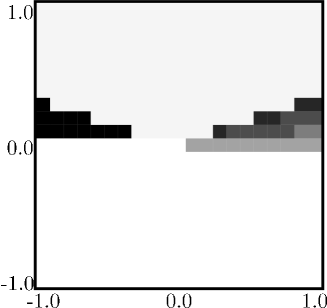
(f) Lutz1, $m=10$

Figure 1: Tuning results presented in graphical form for six representative instances. The y-axis ranges over the values of $\kappa_{1}$, while the x-axis ranges over the values of $\kappa_{2}$. The gray levels of the squares indicate the quality of the algorithm when run with the corresponding setting: the lighter a square is painted, the better is the parameter setting.

4.3 Results

Algorithm Ibs was applied 20 times to all 302 instances. Herefore we used a computation time limit of 180 seconds for each cycle time, that is, Ibs was given maximally 180 seconds for finding a feasible solution for a given cycle time. In case of success, the algorithm has again 180 seconds for the next smaller cycle time, etc. Detailed results of Ibs for all 302 instances are given in Tables 7 and 8 that are to be found in Appendix A. The data is, in both tables, presented as follows. The first two columns provide the name of the precedence graph and the number of work stations ($m$). The third column provides the value of the optimal (respectively, best-known) solutions. In case a value is not proved to be optimal it is overlined. More in detail, in 15 out of 302 cases optimality has not been proved yet. The remaining five columns are reserved for the results of Ibs. The first of these five columns contains the value of the best solution found by Ibs over 20 runs. In case this value is presented with a gray background, a new best-known solution has been found. On the other side, if this value is marked by an asterisk, the obtained result does not reach the value of a best-known solution. In all other cases the values correspond to the values of best-known solutions. The second column provides the average over 20 runs, while the third column contains the corresponding standard deviation. The fourth column gives the average time (in seconds) at which the best solution of a run was found, averaged over 20 runs. The fifth column provides the corresponding standard deviation. From the results presented in Tables 7 and 8 (see Appendix A) we can observe that Ibs obtains best-known (respectively, optimal) solutions in 276 out of 302 cases. Moreover, new best solutions are obtained in 6 cases. This is remarkable as—despite a considerable amount of ongoing research—in the last 14 years no improved solutions have been reported. Only in 20 cases (all concerning precedence graphs Arcus1, Arcus2, Scholl, and Warnecke) our algorithm was not able to find the best solutions known. However, in most of these cases the deviation from the best-known solution is no more than one unit of cycle time.

Table 3: Results of Ibs in comparison to the best (TabuSearch), respectively most recent (DE_rks and PNA-for), methods from the literature.

	DE_rks	PNA-for	TabuSearch	Iterative Beam Search (Ibs)
#opt	n/g	39	168	282
mrd (%)	2.64	2.73	0.40	0.0029
time (s)	10.74	407.28	84.90	31.61
Note: n/g means not given

In addition to Tables 7 and 8 the results of Ibs are presented in a summarized way in Table 3, in comparison to three other algorithms. TabuSearch [22], even though already published in 1996, still counts as the current state-of-the-art heuristic method for SALBP-2. DE_rks is the best version of a differential evolution (DE) algorithm proposed in [14], and PNA-for is a Petri net-based heuristic published in [11]. The last two methods are, to our knowledge, the most recently published heuristic methods for SALBP-2. Three measure are used in Table 3 for the comparison of Ibs with these three algorithms. The row labelled #opt provides the number of best-known solutions found by each method (over 302). Moreover, the row labelled mrd (%) gives the mean relative deviation (in percent) of the results obtained by the four algorithms from the best-known solutions for all 302 instances. Finally, row time contains the average computation time of the algorithms for all 302 instances. Concerning the quality of the results, we can conclude that Ibs clearly outperforms its competitors. For the correct interpretation of the computation times it has to be taken into account that the four algorithms were executed on computers with very different processor speeds. While TabuSearch was executed on a 80486 DX2-66 processor, PNA-for was run on an Athlon XP 2000+ processor with 1.67 GHz, and DE_rks was run on a Pentium IV processor with 1.7 GHz. This means that TabuSearch was run by far on the slowest machine, Ibs by far on the fastest machine, and PNA-for and DE_rks on comparable machines. Given the computation times in Table 3 we can savely conclude that TabuSearch is the fastest algorithm, and PNA-for is the slowest one. However, note that assembly line balancing is, in most cases, not a time-critical application. In other words, for most practical purposes it does not matter if an algorithm takes 1 minute or 6 hours of computation time.

In the following we present the results of Ibs in comparison to DE_rks and PNA-for in the same way as done in [14] and [11]. In these works, results were presented as averages over instances based on the same precedence graph, and also averaged over Dataset1 and Dataset2. The quality of the results is given in terms of the mean relative deviation (in percent) from the best-known solutions. Tables 4 and 5 clearly show that Ibs is largely superior to both competitor algorithms.

Table 4: Results of Ibs in comparison to DE_rks and PNA-for for the 128 instances of Dataset1 (averaged over precedence graphs).

Graph	DE_rks		PNA-for	Iterative Beam Search (Ibs)
	mrd (%)	time (s)	mrd (%)	mrd (%)	time (s)
Buxey	1.16	0.80	3.07	0.0	0.06
Sawyer	2.27	1.64	4.00	0.0	0.14
Lutz1	0.32	0.88	4.09	0.0	0.55
Gunther	0.14	1.08	1.27	0.0	0.02
Kilbridge	0.66	1.43	2.19	0.0	0.0067
Tonge	1.88	3.71	2.53	0.0	7.73
Arcus1	0.99	5.29	2.47	0.0287	152.34
Lutz2	3.08	1.00	2.99	0.0	0.035
Arcus2	4.96	19.02	2.06	0.0066	135.83
Average:	1.72	3.87	2.57	0.0058	51.76

Table 5: Results of Ibs in comparison to DE_rks and PNA-for for the 174 instances of Dataset2 (averaged over precedence graphs).

Graph	DE_rks		PNA-for	Iterative Beam Search (Ibs)
	mrd (%)	time (s)	mrd (%)	mrd (%)	time (s)
Hahn	0.0	1.00	2.52	0.0	0.065
Warnecke	3.74	3.53	5.57	0.0579	1.54
Wee-Mag	1.23	3.68	1.56	0.0	0.65
Lutz3	1.68	5.62	2.59	0.0	0.61
Mukherje	n/a	n/a	1.04	0.0	2.52
Barthold	0.26	19.47	1.02	0.0	0.079
Barthol2	6.85	33.08	3.97	0.0	0.96
Scholl	9.51	43.95	3.21	0.0028	98.69
Average:	3.32	15.79	2.85	0.00071	16.79

4.4 Results of a High-Performance Version

In an attempt to further improve on the results of our algorithm we decided to apply a high-performance version of Ibs to all problem instances for which the optimal solution is unknown and, additionally, to all instances where Ibs—with the settings as outlined in the previous section—was not able to find a best-known solution. This high-performance version is obtained as follows. First, 1800 seconds are used as a time limit for each cycle time. Second, in line 17 of Algorithm 3 only 1% of the time limit is used (instead of 5%). Third, for each application of beam search in lines 18 and 20 of Algorithm 3 the beam width $k_{\text{\tiny bw}}$ is randomly chosen from $[150,250]$ and the number of extensions is randomly chosen from $[20,40]$. Moreover, with a probability of $0.5$ the heuristic information is—for each application of beam search—calculated using the weight values as outlined in Table 1. Otherwise, the weight values are chosen randomly from $[-1,1]$. With these modifications we applied Ibs exactly once to all the instances of Table 6. The results of the algorithm are given in column Result. Indeed, the number of instances for which a best-known solution can not be found before is reduced from 20 to 10 instances. Moreover, the algorithm is now able to find new best-known solutions in 9 (instead of only 6) cases. Summarizing, this amounts to 283 best-known solutions found and 9 new best-known solutions obtained. In one case, (Scholl, $m=49$), the new best-known solution is provenly optimal, as its value coincides with the best known lower bound.

Table 6: Results of a high-performance version of Ibs.

Graph	$m$	Result	Graph	$m$	Result
Arcus1 (83)	8	9554	Arcus2 (111)	23	6560
	11	7085∗		24	6282
	12	6412		25	6101
	17	4527∗		26	5855
	18	4323∗	Scholl (297)	31	2247
	19	4071∗		36	1936∗
	20	3886∗		42	1660∗
Arcus2 (111)	14	10747		46	1515
	15	10035		47	1484∗
	16	9413∗		49	1423
	17	8857∗	Warnecke (58)	25	64
	18	8377	Wee-Mag (75)	18	87
	19	7922		19	85
	20	7524		23	67
	21	7187		27	65
	22	6856		28	64

5 Conclusions and Future Work

In this work we have proposed an iterative beam search algorithm for the simple assembly line balancing problem with a fixed number of work stations, SALBP-2. The experimental evalution of the algorithm has shown that it is currently a state-of-the-art method for this problem. Appart from producing optimal, respectively best-known, solutions in 283 out of 302 test cases, our algorithm generated new best-known solutions in further 9 test cases. Encouraged by the results for the SALBP-1 version of the problem (as published in [3]) and the results obtained in this paper for the SALBP-2 we intent to apply similar algorithms based on beam search to other assembly line balancing problems.

Appendix A

Table 7: Detailed results of Ibs for 302 test instances (Part A).

Graph	$m$	bks	Iterative Beam Search (Ibs)					Graph	$m$	bks	Iterative Beam Search (Ibs)
			best	avg	std	time (s)	std				best	avg	std	time (s)	std
Arcus1 (83)	3	25236	25236	25236.00	(0.00)	0.56	(0.29)	Barthold (148)	9	626	626	626.00	(0.00)	0.13	(0.03)
	4	18927	18927	18927.00	(0.00)	6.16	(3.92)		10	564	564	564.00	(0.00)	0.10	(0.02)
	5	15142	15142	15142.00	(0.00)	80.08	(16.69)		11	513	513	513.00	(0.00)	0.09	(0.00)
	6	12620	12620	12620.00	(0.00)	15.52	(5.76)		12	470	470	470.00	(0.00)	0.09	(0.00)
	7	10826	10826	10826.00	(0.00)	59.80	(19.89)		13	434	434	434.00	(0.00)	0.16	(0.02)
	8	9554	∗9555	9555.55	(0.51)	120.54	(63.16)		14	403	403	403.00	(0.00)	0.14	(0.01)
	9	8499	8499	8500.70	(0.80)	130.73	(117.23)		15	383	383	383.00	(0.00)	0.05	(0.00)
	10	7580	7580	7580.95	(0.60)	311.89	(109.87)	Buxey (29)	7	47	47	47.00	(0.00)	0.46	(0.51)
	11	7084	∗7086	7086.70	(0.47)	71.13	(52.77)		8	41	41	41.00	(0.00)	0.00	(0.00)
	12	6412	∗6413	6414.10	(0.72)	362.32	(66.26)		9	37	37	37.00	(0.00)	0.01	(0.00)
	13	5864	5864	5864.00	(0.00)	129.18	(12.99)		10	34	34	34.00	(0.00)	0.00	(0.00)
	14	5441	5441	5441.00	(0.00)	2.02	(0.41)		11	32	32	32.00	(0.00)	0.00	(0.00)
	15	5104	5104	5104.45	(0.60)	222.29	(73.92)		12	28	28	28.00	(0.00)	0.01	(0.00)
	16	4850	4850	4850.00	(0.00)	33.84	(9.59)		13	27	27	27.00	(0.00)	0.01	(0.00)
	17	4516	∗4524	4526.20	(0.89)	282.49	(100.96)		14	25	25	25.00	(0.00)	0.00	(0.00)
	18	4317	∗4322	4323.20	(0.77)	291.73	(111.23)	Gunther (35)	6	84	84	84.00	(0.00)	0.00	(0.00)
	19	4068	∗4073	4074.80	(1.01)	326.78	(125.49)		7	72	72	72.00	(0.00)	0.03	(0.00)
	20	3882	∗3886	3889.25	(2.05)	594.21	(204.09)		8	63	63	63.00	(0.00)	0.01	(0.00)
	21	3691	3691	3691.00	(0.00)	5.58	(0.81)		9	54	54	54.00	(0.00)	0.05	(0.04)
	22	3691	3691	3691.00	(0.00)	0.02	(0.00)		10	50	50	50.00	(0.00)	0.01	(0.00)
Arcus2 (111)	3	50133	50133	50133.00	(0.00)	0.09	(0.03)		11	48	48	48.00	(0.00)	0.00	(0.00)
	4	37600	37600	37600.00	(0.00)	0.41	(0.02)		12	44	44	44.00	(0.00)	0.01	(0.00)
	5	30080	30080	30080.00	(0.00)	0.43	(0.22)		13	42	42	42.00	(0.00)	0.01	(0.00)
	6	25067	25067	25067.00	(0.00)	1.13	(0.59)		14	40	40	40.00	(0.00)	0.02	(0.00)
	7	21486	21486	21486.00	(0.00)	1.76	(1.04)		15	40	40	40.00	(0.00)	0.01	(0.00)
	8	18800	18800	18800.00	(0.00)	11.36	(2.86)	Hahn (53)	3	4787	4787	4787.00	(0.00)	0.00	(0.00)
	9	16711	16711	16711.00	(0.00)	28.03	(12.51)		4	3677	3677	3677.00	(0.00)	0.08	(0.01)
	10	15040	15040	15040.00	(0.00)	38.67	(15.08)		5	2823	2823	2823.00	(0.00)	0.01	(0.00)
	11	13673	13673	13673.00	(0.00)	49.47	(12.83)		6	2400	2400	2400.00	(0.00)	0.05	(0.01)
	12	12534	12534	12534.00	(0.00)	43.34	(15.17)		7	2336	2336	2336.00	(0.00)	0.29	(0.01)
	13	11570	11570	11570.00	(0.00)	32.60	(14.63)		8	1907	1907	1907.00	(0.00)	0.09	(0.03)
	14	10747	∗10748	10748.00	(0.00)	62.69	(16.17)		9	1827	1827	1827.00	(0.00)	0.00	(0.00)
	15	10035	∗10036	10036.40	(0.50)	112.54	(63.37)		10	1775	1775	1775.00	(0.00)	0.00	(0.00)
	16	9412	∗9416	9416.60	(0.68)	290.35	(90.83)	Kilbridge (45)	3	184	184	184.00	(0.00)	0.00	(0.00)
	17	8855	∗8864	8864.90	(0.31)	87.41	(52.86)		4	138	138	138.00	(0.00)	0.01	(0.00)
	18	$\overline{8377}$	8377	8377.00	(0.00)	8.11	(1.00)		5	111	111	111.00	(0.00)	0.00	(0.00)
	19	$\overline{7928}$	7924	7925.60	(0.60)	205.09	(76.12)		6	92	92	92.00	(0.00)	0.00	(0.00)
	20	$\overline{7526}$	7524	7524.40	(0.50)	159.72	(57.92)		7	79	79	79.00	(0.00)	0.01	(0.00)
	21	$\overline{7188}$	∗7192	7193.40	(0.82)	318.78	(89.64)		8	69	69	69.00	(0.00)	0.01	(0.00)
	22	$\overline{6859}$	6858	6858.20	(0.41)	226.94	(75.52)		9	62	62	62.00	(0.00)	0.01	(0.00)
	23	$\overline{6561}$	6560	6563.10	(1.45)	428.68	(168.53)		10	56	56	56.00	(0.00)	0.01	(0.00)
	24	$\overline{6289}$	6284	6285.65	(1.46)	311.77	(144.55)		11	55	55	55.00	(0.00)	0.01	(0.00)
	25	$\overline{6106}$	∗6112	6114.15	(0.99)	305.50	(90.99)	Lutz1 (32)	8	1860	1860	1860.00	(0.00)	0.14	(0.00)
	26	$\overline{5856}$	∗5858	5860.45	(1.76)	661.48	(192.47)		9	1638	1638	1638.00	(0.00)	2.41	(0.34)
	27	5689	5689	5689.00	(0.00)	9.29	(0.17)		10	1526	1526	1526.00	(0.00)	0.18	(0.01)
Barthol2 (148)	27	157	157	157.00	(0.00)	0.31	(0.03)		11	1400	1400	1400.00	(0.00)	0.01	(0.00)
	28	152	152	152.00	(0.00)	0.44	(0.07)		12	1400	1400	1400.00	(0.00)	0.00	(0.00)
	29	146	146	146.00	(0.00)	0.80	(0.32)	Lutz2 (89)	9	54	54	54.00	(0.00)	0.02	(0.01)
	30	142	142	142.00	(0.00)	0.15	(0.03)		10	49	49	49.00	(0.00)	0.03	(0.00)
	31	137	137	137.00	(0.00)	0.67	(0.09)		11	45	45	45.00	(0.00)	0.04	(0.00)
	32	133	133	133.00	(0.00)	0.57	(0.07)		12	41	41	41.00	(0.00)	0.03	(0.00)
	33	129	129	129.00	(0.00)	0.52	(0.06)		13	38	38	38.00	(0.00)	0.03	(0.00)
	34	125	125	125.00	(0.00)	0.47	(0.05)		14	35	35	35.00	(0.00)	0.03	(0.00)
	35	121	121	121.00	(0.00)	0.94	(0.15)		15	33	33	33.00	(0.00)	0.03	(0.00)
	36	118	118	118.00	(0.00)	0.87	(0.11)		16	31	31	31.00	(0.00)	0.02	(0.00)
	37	115	115	115.00	(0.00)	0.92	(0.19)		17	29	29	29.00	(0.00)	0.04	(0.00)
	38	112	112	112.00	(0.00)	0.76	(0.06)		18	28	28	28.00	(0.00)	0.04	(0.00)
	39	109	109	109.00	(0.00)	0.70	(0.13)		19	26	26	26.00	(0.00)	0.04	(0.01)
	40	106	106	106.00	(0.00)	0.91	(0.32)		20	25	25	25.00	(0.00)	0.04	(0.00)
	41	104	104	104.00	(0.00)	0.72	(0.05)		21	24	24	24.00	(0.00)	0.02	(0.00)
	42	101	101	101.00	(0.00)	2.77	(5.43)		22	23	23	23.00	(0.00)	0.04	(0.00)
	43	99	99	99.00	(0.00)	0.84	(0.23)		23	22	22	22.00	(0.00)	0.05	(0.00)
	44	97	97	97.00	(0.00)	0.59	(0.15)		24	21	21	21.00	(0.00)	0.05	(0.00)
	45	95	95	95.00	(0.00)	0.76	(0.25)		25	20	20	20.00	(0.00)	0.02	(0.00)
	46	93	93	93.00	(0.00)	0.68	(0.29)		26	19	19	19.00	(0.00)	0.05	(0.02)
	47	91	91	91.00	(0.00)	0.67	(0.15)		27	19	19	19.00	(0.00)	0.03	(0.00)
	48	89	89	89.00	(0.00)	1.17	(0.47)		28	18	18	18.00	(0.00)	0.05	(0.00)
	49	87	87	87.00	(0.00)	0.83	(0.26)	Lutz3 (89)	3	548	548	548.00	(0.00)	0.01	(0.00)
	50	85	85	85.90	(0.31)	3.28	(10.33)		4	411	411	411.00	(0.00)	0.03	(0.00)
	51	84	84	84.00	(0.00)	2.60	(2.09)		5	329	329	329.00	(0.00)	0.01	(0.00)
Barthold (148)	3	1878	1878	1878.00	(0.00)	0.01	(0.00)		6	275	275	275.00	(0.00)	0.01	(0.00)
	4	1409	1409	1409.00	(0.00)	0.02	(0.00)		7	236	236	236.00	(0.00)	0.02	(0.00)
	5	1127	1127	1127.00	(0.00)	0.02	(0.00)		8	207	207	207.00	(0.00)	0.04	(0.00)
	6	939	939	939.00	(0.00)	0.06	(0.01)		9	184	184	184.00	(0.00)	5.54	(4.14)
	7	805	805	805.00	(0.00)	0.11	(0.00)		10	165	165	165.00	(0.00)	0.09	(0.01)
	8	705	705	705.00	(0.00)	0.04	(0.01)		11	151	151	151.00	(0.00)	0.06	(0.00)

Table 8: Detailed results of Ibs for 302 test instances (Part B).

Graph	$m$	bks	Iterative Beam Search (Ibs)					Graph	$m$	bks	Iterative Beam Search (Ibs)
			best	avg	std	time (s)	std				best	avg	std	time (s)	std
Lutz3 (89)	12	138	138	138.00	(0.00)	0.02	(0.00)	Tonge (70)	6	585	585	585.00	(0.00)	0.03	(0.02)
	13	128	128	128.00	(0.00)	0.05	(0.03)		7	502	502	502.00	(0.00)	0.06	(0.01)
	14	118	118	118.00	(0.00)	0.67	(0.52)		8	439	439	439.00	(0.00)	0.04	(0.01)
	15	110	110	110.00	(0.00)	0.80	(0.66)		9	391	391	391.00	(0.00)	0.05	(0.00)
	16	105	105	105.00	(0.00)	0.34	(0.30)		10	352	352	352.00	(0.00)	0.06	(0.01)
	17	98	98	98.00	(0.00)	0.19	(0.05)		11	320	320	320.00	(0.00)	0.06	(0.02)
	18	93	93	93.00	(0.00)	0.16	(0.05)		12	294	294	294.00	(0.00)	0.09	(0.01)
	19	89	89	89.00	(0.00)	0.05	(0.03)		13	271	271	271.00	(0.00)	0.06	(0.01)
	20	85	85	85.00	(0.00)	0.14	(0.05)		14	251	251	251.80	(0.41)	20.25	(45.26)
	21	80	80	80.00	(0.00)	0.11	(0.02)		15	235	235	235.00	(0.00)	0.35	(0.16)
	22	76	76	76.00	(0.00)	4.20	(3.30)		16	221	221	221.00	(0.00)	0.97	(0.93)
	23	74	74	74.00	(0.00)	0.29	(0.18)		17	208	208	208.00	(0.00)	1.02	(0.95)
Mukherje (94)	3	1403	1403	1403.00	(0.00)	0.01	(0.00)		18	196	196	196.15	(0.37)	46.76	(39.05)
	4	1052	1052	1052.00	(0.00)	0.10	(0.00)		19	186	186	186.35	(0.49)	87.09	(64.62)
	5	844	844	844.00	(0.00)	0.02	(0.00)		20	177	177	177.90	(0.31)	9.46	(39.39)
	6	704	704	704.00	(0.00)	0.02	(0.00)		21	170	170	170.00	(0.00)	8.71	(9.43)
	7	621	621	621.00	(0.00)	0.12	(0.00)		22	162	162	162.00	(0.00)	2.52	(2.45)
	8	532	532	532.00	(0.00)	0.09	(0.01)		23	156	156	156.00	(0.00)	0.11	(0.04)
	9	471	471	471.00	(0.00)	0.09	(0.01)		24	156	156	156.00	(0.00)	0.02	(0.00)
	10	424	424	424.00	(0.00)	0.02	(0.00)		25	156	156	156.00	(0.00)	0.02	(0.00)
	11	391	391	391.00	(0.00)	0.10	(0.01)	Warnecke (58)	3	516	516	516.00	(0.00)	0.02	(0.00)
	12	358	358	358.00	(0.00)	0.05	(0.01)		4	387	387	387.00	(0.00)	0.08	(0.08)
	13	325	325	325.00	(0.00)	0.17	(0.06)		5	310	310	310.00	(0.00)	0.03	(0.00)
	14	311	311	311.00	(0.00)	0.08	(0.01)		6	258	258	258.00	(0.00)	0.10	(0.06)
	15	288	288	288.00	(0.00)	0.09	(0.02)		7	222	222	222.00	(0.00)	0.03	(0.00)
	16	268	268	268.00	(0.00)	0.20	(0.02)		8	194	194	194.00	(0.00)	0.05	(0.01)
	17	251	251	251.00	(0.00)	0.45	(0.05)		9	172	172	172.00	(0.00)	2.40	(2.28)
	18	239	239	239.00	(0.00)	0.24	(0.02)		10	155	155	155.00	(0.00)	0.05	(0.01)
	19	226	226	226.00	(0.00)	0.03	(0.01)		11	142	142	142.00	(0.00)	0.04	(0.00)
	20	220	220	220.05	(0.22)	57.07	(43.23)		12	130	130	130.00	(0.00)	0.07	(0.01)
	21	208	208	208.00	(0.00)	0.12	(0.00)		13	120	120	120.00	(0.00)	0.08	(0.01)
	22	200	200	200.00	(0.00)	0.13	(0.06)		14	111	111	111.00	(0.00)	0.29	(0.24)
	23	189	189	189.00	(0.00)	0.12	(0.02)		15	104	104	104.00	(0.00)	0.27	(0.13)
	24	179	179	179.00	(0.00)	0.48	(0.41)		16	98	98	98.00	(0.00)	0.08	(0.01)
	25	172	172	172.00	(0.00)	0.43	(0.18)		17	92	92	92.00	(0.00)	0.26	(0.14)
	26	171	171	171.00	(0.00)	0.27	(0.03)		18	87	87	87.00	(0.00)	0.27	(0.14)
Sawyer (30)	7	47	47	47.00	(0.00)	0.14	(0.11)		19	84	84	84.00	(0.00)	0.10	(0.06)
	8	41	41	41.00	(0.00)	0.06	(0.03)		20	79	79	79.00	(0.00)	0.13	(0.03)
	9	37	37	37.00	(0.00)	0.03	(0.01)		21	76	76	76.00	(0.00)	0.08	(0.04)
	10	34	34	34.00	(0.00)	0.02	(0.00)		22	73	73	73.00	(0.00)	0.53	(0.36)
	11	31	31	31.00	(0.00)	0.82	(0.85)		23	69	69	69.00	(0.00)	18.10	(21.25)
	12	28	28	28.00	(0.00)	0.03	(0.01)		24	66	66	66.90	(0.31)	2.88	(9.10)
	13	26	26	26.00	(0.00)	0.02	(0.00)		25	64	∗65	65.00	(0.00)	12.30	(11.87)
	14	25	25	25.00	(0.00)	0.02	(0.00)		26	64	64	64.00	(0.00)	0.05	(0.01)
Scholl (297)	25	2787	2787	2787.00	(0.00)	37.11	(6.11)		27	60	60	60.00	(0.00)	1.61	(0.73)
	26	2680	2680	2680.00	(0.00)	32.56	(4.71)		28	59	59	59.00	(0.00)	0.16	(0.06)
	27	2580	2580	2580.00	(0.00)	58.06	(8.65)		29	56	56	56.00	(0.00)	1.43	(1.15)
	28	2488	2488	2488.00	(0.00)	53.78	(12.43)	Wee-Mag (75)	3	500	500	500.00	(0.00)	0.01	(0.00)
	29	2402	2402	2402.00	(0.00)	45.57	(9.93)		4	375	375	375.00	(0.00)	0.03	(0.00)
	30	2322	2322	2322.30	(0.47)	96.86	(53.36)		5	300	300	300.00	(0.00)	0.02	(0.00)
	31	2247	∗2248	2248.00	(0.00)	51.23	(4.32)		6	250	250	250.00	(0.00)	0.03	(0.00)
	32	2177	2177	2177.50	(0.51)	91.50	(63.17)		7	215	215	215.00	(0.00)	0.01	(0.00)
	33	2111	2111	2111.80	(0.41)	57.19	(39.95)		8	188	188	188.00	(0.00)	0.04	(0.01)
	34	2049	2049	2049.20	(0.41)	117.47	(53.03)		9	167	167	167.00	(0.00)	0.01	(0.00)
	35	1991	1991	1991.00	(0.00)	95.54	(17.19)		10	150	150	150.00	(0.00)	0.08	(0.02)
	36	1935	∗1936	1936.00	(0.00)	61.22	(8.78)		11	137	137	137.00	(0.00)	0.06	(0.01)
	37	1883	1883	1883.05	(0.22)	140.57	(34.46)		12	125	125	125.00	(0.00)	0.10	(0.02)
	38	1834	1834	1834.00	(0.00)	125.92	(34.53)		13	116	116	116.00	(0.00)	0.02	(0.00)
	39	1787	1787	1787.35	(0.49)	192.12	(55.85)		14	108	108	108.00	(0.00)	0.54	(0.60)
	40	1742	1742	1742.00	(0.00)	153.02	(29.66)		15	100	100	100.00	(0.00)	0.24	(0.19)
	41	1700	1700	1700.00	(0.00)	81.51	(18.06)		16	94	94	94.00	(0.00)	0.05	(0.01)
	42	1659	∗1660	1660.00	(0.00)	146.58	(32.11)		17	89	89	89.00	(0.00)	0.42	(0.28)
	43	1621	1621	1621.00	(0.00)	149.08	(21.75)		18	$\overline{87}$	87	87.00	(0.00)	0.07	(0.01)
	44	1584	1584	1584.15	(0.37)	127.52	(54.06)		19	$\overline{85}$	85	85.00	(0.00)	0.08	(0.02)
	45	1549	1549	1549.00	(0.00)	150.65	(32.59)		20	77	77	77.00	(0.00)	0.13	(0.04)
	46	1515	∗1516	1516.00	(0.00)	121.28	(20.06)		21	72	72	72.00	(0.00)	0.08	(0.01)
	47	1483	∗1484	1484.00	(0.00)	165.44	(28.64)		22	69	69	69.00	(0.00)	0.06	(0.01)
	48	1452	1452	1452.70	(0.47)	151.98	(60.76)		23	$\overline{67}$	67	67.00	(0.00)	4.34	(3.58)
	49	$\overline{1427}$	1424	1424.00	(0.00)	113.46	(22.47)		24	66	66	66.00	(0.00)	0.25	(0.14)
	50	1394	1394	1394.85	(0.37)	143.63	(53.48)		25	65	65	65.00	(0.00)	11.36	(26.58)
	51	1386	1386	1386.00	(0.00)	2.23	(0.09)		26	65	65	65.00	(0.00)	0.05	(0.01)
	52	1386	1386	1386.00	(0.00)	0.17	(0.01)		27	$\overline{65}$	65	65.00	(0.00)	0.02	(0.00)
Tonge (70)	3	1170	1170	1170.00	(0.00)	0.01	(0.00)		28	$\overline{64}$	64	64.00	(0.00)	0.02	(0.00)
	4	878	878	878.00	(0.00)	0.02	(0.00)		29	63	63	63.00	(0.00)	0.02	(0.00)
	5	702	702	702.00	(0.00)	0.05	(0.02)		30	56	56	56.00	(0.00)	0.07	(0.00)

References

- [1] H. Akeba, M. Hifib, and R. M’Hallah. A beam search algorithm for the circular packing problem. Computers & Operations Research, 36(5):1513–1528, 2009.
- [2] E. J. Anderson and M. C. Ferris. Genetic algorithms for combinatorial optimization: The assembly line balancing problem. ORSA Journal on Computing, 6:161–173, 1994.
- [3] C. Blum. Beam-ACO for simple assembly line balancing. INFORMS Journal on Computing, 20(4):618–627, 2008.
- [4] C. Blum, M. J. Blesa, and M. López Ibáñez. Beam search for the longest common subsequence problem. Computers & Operations Research, 36(12):3178–3186, 2009.
- [5] C. Blum and C. Miralles. On solving the assembly line worker assignment and balancing problem via beam search. Computers & Operations Research, 38(1):328–339, 2011.
- [6] W.-C. Chiang. The application of a tabu search metaheuristic to the assembly line balancing problem. Annals of Operations Research, 77:209–227, 1998.
- [7] M. Ghirardi and C. N. Potts. Makespan minimization for scheduling unrelated parallel machines: A recovering beam search approach. European Journal of Operational Research, 165(2):457–467, 2005.
- [8] S. Gosh and R. J. Gagnon. A comprehensive literature review and analysis of the design, balancing and scheduling of assembly systems. International Journal of Production Research, 27:637–670, 1989.
- [9] S. T. Hackman, M. J. Magazine, and T. S. Wee. Fast, effective algorithms for simple assembly line balancing problems. Operations Research, 37:916–924, 1989.
- [10] A. Henrici. A comparison between simulated annealing and tabu search with an example from the production planning. In H. Dyckhoff et al., editor, Operations Research Proceedings, pages 498–503. Springer Verlag, Berlin, Germany, 1994.
- [11] O. Kilincci. A Petri net-based heuristic for simply assembly line balancing problem of type 2. International Journal of Advanced Manufacturing Technology, 46:329–338, 2010.
- [12] R. Klein and A. Scholl. Maximizing the production rate in simple assembly line balancing—A branch and bound procedure. European Journal of Operational Research, 91:367–385, 1996.
- [13] G.-C. Lee and D. L. Woodruff. Beam search for peak alignment of NMR signals. Analytica Chimica Acta, 513(2):413–416, 2004.
- [14] A. C. Nearchou. Balancing large assembly lines by a new heuristic based on differential evolution. International Journal of Advanced Manufacturing Technology, 34:1016–1029, 2007.
- [15] P. S. Ow and T. E. Morton. Filtered beam search in scheduling. International Journal of Production Research, 26:297–307, 1988.
- [16] R. Pastor, L. Ferrer, and A. García. Evaluating optimization models to solve SALBP. In O. Gervasi and M. L. Gavrilova, editors, Proceedings of ICCSA 2007 – International Conference on Computational Science and Its Applications, volume 4705 of Lecture Notes in Computer Science, pages 791–803. Springer Verlag, Berlin, Germany, 2007.
- [17] I. Sabuncuoglu and M. Bayiz. Job shop scheduling with beam search. European Journal of Operational Research, 118:390–412, 1999.
- [18] M. E. Salveson. The assembly line balancing problem. Journal of Industrial Engineering, 6:18–25, 1955.
- [19] A. Scholl. Ein B&B-Verfahren zur Abstimmung von Einprodukt-Fließbändern bei gegebener Stationsanzahl. In H. Dyckhoff et al., editor, Operations Research Proceedings, pages 175–181. Springer Verlag, Berlin, Germany, 1994.
- [20] A. Scholl. Balancing and sequencing assembly lines. Physica Verlag, Heidelberg, Germany, 2nd edition edition, 1999.
- [21] A. Scholl and C. Becker. State-of-the-art exact and heuristic solution procedures for simple assembly line balancing. European Journal of Operational Research, 168(3):666–693, 2006.
- [22] A. Scholl and S. Voss. Simple assembly line balancing—Heuristic approaches. Journal of Heuristics, 2:217–244, 1996.
- [23] H. F. Ugurdag, R. Rachamadugu, and C. A. Papachristou. Designing paced assembly lines with fixed number of stations. European Journal of Operational Research, 102:488–501, 1997.
- [24] J. M. S. Valente and R. A. F. S. Alves. Filtered and recovering beam search algorithms for the early/tardy scheduling problem with no idle time. Computers & Industrial Engineering, 48(2):363–375, 2005.
- [25] T. Watanabe, Y. Hashimoto, L. Nishikawa, and H. Tokumaru. Line balancing using a genetic evolution model. Control Engineering Practice, 3:69–76, 1995.