Chiral Magnetic Effect from Q-balls

Abstract

We apply a generic framework of linear sigma models for revealing a mechanism of the mysterious phenomenon, the chiral magnetic effect, in quark-gluon plasma. An electric current arises along a background magnetic field, which is given rise to by Q-balls (non-topological solitons) of the linear sigma model with axial anomaly. We find additional alternating current due to quark mass terms. The hadronic Q-balls, baby boson stars, may be created in heavy-ion collisions.

It is widely believed that QCD has a phase transition between the hadronic phase and the quark-gluon plasma (QGP) phase at finite temperature and density. Experimental searches for QGP in relativistic heavy ion collisions have been revealed that QGP has highly nontrivial properties, such as its perfect fluidity Huovinen:2001cy ; Adler:2003kt ; Adams:2003am , for example. The chiral magnetic effect (CME) Kharzeev:2007jp ; Fukushima:2008xe is one of the most striking phenomena in QGP which has been recently studied from the theoretical and experimental viewpoints. The CME, the separation of electric charge along the axis of an external electromagnetic fields, was predicted as a direct evidence of the (not global but local) strong CP violation under very intense external magnetic fields, and was observed in heavy ion collisions. Recently, an experimental evidence was presented by the STAR Collaboration at RHIC Voloshin:2009hr . Since the discovery of the evidence, CME has been actively studied using non-perturbative techniques in QCD: P-NJL model Fukushima:2010fe , holographic QCD Rebhan:2009vc , lattice QCD Buividovich:2009wi , and so on.

In this short note, in order to understand CME in QGP, we consider a generic linear sigma model (LSM) which is widely used as a key tool to understand the phase transitions. We find a universal mechanism for CME which is given rise to by a stable non-topological solitonic configuration of the (pseudo-)scalar mesons, so-called Q-ball Coleman:1985ki . Interior of the Q-ball is in the hadronic phase where the scalar mesons condense, while it is QGP outside the Q-ball. We find that the electric current along the external magnetic field arises in a similar manner discussed in literature. In addition, as a consequence of the Q-ball, the electric current not only is a direct current but also has a small alternating current from quark mass terms.

The generic LSM of the scalar mesons $\Phi_{ij}=\bar{q}_{\rm R}^{j}q_{\rm L}^{i}$ is given by

$${\cal L}_{\rm eff}={\rm Tr}\left[\partial_{\mu}\Phi\partial^{\mu}\Phi^{\dagger}-M(\Phi+\Phi^{\dagger})\right]-V(\Phi\Phi^{\dagger})$$

$$+A\left(\det\Phi+\det\Phi^{\dagger}\right),$$ (1)

where the metric is taken to be $\eta_{\mu\nu}={\rm diag}(+,-,-,-)$. The matrix $M$ is proportional to the quark mass matrix $M\propto{\rm diag}(m_{\rm u},m_{\rm d},m_{\rm s})$, and the last term is a manifestation of the $U(1)_{\rm A}$ anomaly in QCD. This Lagrangian enjoys the same symmetries as QCD. $\Phi$ is singlet under $SU(3)_{\rm C}\times U(1)_{\rm B}$. The chiral $SU(3)_{\rm L}\times SU(3)_{\rm R}$ symmetry and $U(1)_{\rm A}$ acts on $\Phi$ as $\Phi\to e^{i\alpha}U_{\rm L}\Phi U_{\rm R}^{\dagger}$, which are the exact symmetries if $M=0$ and $A=0$. The currents corresponding to the axial part of these symmetries $\Phi\to e^{i\alpha}U\Phi U$, are given by $J_{\mu}^{5,a}=i{\rm Tr}[T^{a}(\Phi\partial_{\mu}\Phi^{\dagger}+\partial_{\mu}\Phi^{\dagger}\Phi-\Phi^{\dagger}\partial_{\mu}\Phi-\partial_{\mu}\Phi\Phi^{\dagger})]$, where $\lambda^{a}=2T^{a}$ $(a=1,\ldots,8)$ are the Gell-Mann matrices for flavor $SU(3)$ and $T^{0}={1\over\sqrt{6}}{\boldsymbol{1}}_{3}$.

In order to discuss CME, we consider the electromagnetic field. The electromagnetic couplings of the quarks in QCD give rise to additional anomalies for the diagonal elements of the axial currents, $J_{\mu}^{5,a=0,3,8}$. From the effective theory point of view, these anomalies generate couplings between the diagonal pseudo-scalars and the electromagnetic field. Our idea for the mechanism of CME is that non-trivial background for the diagonal pseudo-scalars results in the electric current through these anomalous couplings.

Motivated by such an idea, we concentrate on the diagonal pseudo-scalars and the overall $\sigma$ field. Namely, we restrict $\Phi$ as $\Phi={\rm diag}(\Phi_{1},\Phi_{2},\Phi_{3})=\sigma e^{i\eta^{\prime}T^{0}+i\pi^{0}T^{3}+i\eta T^{8}}$. Then the Lagrangian ${\cal L}_{\rm eff}$ of the LSM, before coupled to the electromagnetism, is simplified to

$$\sum_{i}\!\big{(}|\partial_{\mu}\Phi_{i}|^{2}-M_{ii}(\Phi_{i}+\Phi_{i}^{\ast})\big{)}-V\big{(}|\Phi_{i}|^{2}\big{)}+A\Big{(}\!\prod_{i}\!\Phi_{i}+\!\prod_{i}\!\Phi_{i}^{\ast}\!\Big{)}.$$

If $M_{ii}=A=0$, this model respects the $U(1)_{{\rm L}-{\rm R}}^{3}$ part of the axial $U(3)_{{\rm L}-{\rm R}}$ symmetry. The corresponding current conservation laws $\partial^{\mu}J^{5,a}_{\mu}=0$ ($a=0,3,8$) follow from the equation of motion, where the explicit forms of the currents are given by $J_{\mu}^{5,a}=2i\Sigma_{i}T^{a}_{ii}(\Phi_{i}\partial_{\mu}\Phi^{\ast}_{i}-\Phi^{\ast}_{i}\partial_{\mu}\Phi_{i})$.

Next we couple the electromagnetic field to this system. Since all the scalars we are considering are neutral, the only possible couplings are the anomalous ones explained above. The explicit forms of such terms can be found by requiring that they should contribute to the anomalous current conservation law correctly. Our proposal is

$${\cal L}_{5\!\!\!/} = \frac{3ie^{2}}{32\pi^{2}}F_{\mu\nu}\tilde{F}^{\mu\nu}\ \sum_{i}q_{i}^{2}(\log\Phi_{i}-\log\Phi_{i}^{\ast})$$ (2)

$$= \frac{3e^{2}}{16\pi^{2}}\epsilon^{\mu\nu\rho\sigma}P_{\mu}A_{\nu}F_{\rho\sigma},$$

where $\tilde{F}^{\mu\nu}=\frac{1}{2}\epsilon^{\mu\nu\rho\sigma}F_{\rho\sigma}$ ($\epsilon^{0123}=1$) and each $q_{i}$ is the $i$-th element of the electric charge matrix for $({\rm u,d,s})$ 3-flavors, ${\rm diag}({2\over 3},-{1\over 3},-{1\over 3})$. We have introduced $P_{\mu}=(P_{0},\vec{P})\equiv\partial_{\mu}{\rm Im}\left(\sum_{i}q_{i}^{2}\log\Phi_{i}\right)$ and ignored the total derivative term in the right-most hand. With this term, the anomalous current conservation law is derived by using the Euler-Lagrange equation for $\Phi_{i}$ following from ${\cal L}_{\rm eff}+{\cal L}_{5\!\!\!/}$,

$$\partial_{\mu}J^{\mu a}_{5} \!\!=\!\! \sum_{j}T^{a}_{jj}\Big{(}-\frac{3e^{2}}{8\pi^{2}}q_{j}^{2}F_{\mu\nu}\tilde{F}^{\mu\nu}-2iM_{jj}(\Phi_{j}-\Phi_{j}^{\ast})\Big{)}$$ (3)

$$+\sqrt{6}iA\Big{(}\prod_{i}\Phi_{i}-\prod_{i}\Phi_{i}^{*}\Big{)}\delta^{a0}.$$

Once we restrict $\Phi$ to the pseudo-scalar neutral mesons ($\eta^{\prime}$, $\pi_{0}$ and $\eta$), this reproduces the standard known form of the anomalous law.

As mentioned above, the additional interaction ${\cal L}_{\rm 5\!\!\!/}$ plays a role of an extraordinary source for the electromagnetic field $((-1/2)A_{\mu}{\cal J}^{\mu})$:

$${\cal J}^{\mu}=-\frac{3e^{2}}{4\pi^{2}}P_{\nu}\tilde{F}^{\nu\mu}.$$ (4)

The Maxwell equations derived from the full Lagrangian including the Maxwell term, $-{1\over 4}F_{\mu\nu}F^{\mu\nu}+{\cal L}_{\rm eff}+{\cal L}_{\rm 5\!\!\!/}$; are modified indeed,

$$\vec{\nabla}\times\vec{B}-\frac{\partial\vec{E}}{\partial t}=\vec{J}_{\rm em}+\vec{\cal J},\qquad\vec{\nabla}\cdot\vec{E}=\rho_{\rm em}+{\cal J}_{0}.$$ (5)

with $\vec{\nabla}\times\vec{E}+\frac{\partial\vec{B}}{\partial t}=0$ and $\vec{\nabla}\cdot\vec{B}=0$. Here $J_{\rm em}^{\mu}=(\rho_{\rm em},\vec{J}_{\rm em})$ stands for the usual electric current, which vanishes for our model with the charge-neutral scalars. Thus the triangle anomaly in QCD results in the electromagnetic currents.

Note that these modified Maxwell equations are formally identical to those in the Maxwell-Chern-Simons theory Kharzeev:2009fn if the small fluctuation of $\theta$ in Kharzeev:2009fn is replaced by our LSM field $\Phi$. Furthermore, relation between CME and axion strings and domain walls was studied in Gorsky:2010dr . It has been proposed that CME occurs once the $\theta$ parameter locally fluctuates Kharzeev:2007jp ; Fukushima:2008xe . Since current experiments suggest that the $\theta$ parameter in the bare QCD Lagrangian is very small $\lesssim 10^{-10}$ Baker:2006ts , the origin of such a fluctuation is attributed to the effect of the medium in the QGP phase.

In our approach with the generic LSM, on the other hand, CME is triggered by the Q-balls Coleman:1985ki of the LSM field $\Phi$, which are stable finite-size non-topological solitons. In the following, we shall show that the current of the CME is given by a typical frequency $\omega$ attributed to the Q-ball, as will be found in (10). Note that our argument is independent of the locally fluctuating $\theta$ mentioned above.

In order to prevent inessential complexities, hereafter we will consider one-flavor model

$${\cal L} =-\frac{1}{4}F_{\mu\nu}F^{\mu\nu}\!+\!|\partial_{\mu}\Phi|^{2}\!-\!V(|\Phi|^{2})\!+\!h(\Phi+\Phi^{*})\!-\!\frac{1}{2}A_{\mu}{\cal J}^{\mu},$$

where ${\cal J}^{\mu}\!=\!-\frac{3e^{2}}{4\pi^{2}}\tilde{F}^{\nu\mu}\partial_{\nu}{\rm Im}\left(q^{2}\log\Phi\right)$ and $h$ includes both the quark mass term $M$ and the anomaly term $A$. This Lagrangian has $U(1)_{\rm A}$ symmetry if the last two terms vanish. Let us first construct the Q-ball in $h=0$ limit. We deal with the electromagnetic field as a background field. The Q-ball’s charge, Q-charge, is the axial charge in this one-flavor model.

The existence of Q-balls does not depend on the details of the system Coleman:1985ki . One requirement is that the scalar potential $V(\sigma^{2})$ has a true vacuum at $\sigma=0$ (QGP) as is given in Fig. 2.

Figure 1: A typical form of the scalar potential $V$. There is a true vacuum at $\sigma=0$ (QGP).

Figure 2: The short-dashed line is a typical form of $U$ which allows the Q-ball. The solid line is the special case in which the two extremal values coincide, $U(0)=U(\sigma_{0})=0$.

Let us make the following ansatz for a spherically symmetric $\eta^{\prime}$-ball

$$\Phi=\sigma(r)e^{i\eta^{\prime}(t)},\qquad\eta^{\prime}(t)=\omega t,$$ (6)

with $r=|\vec{x}|$. The Euler-Lagrange equation for the profile function $\sigma$ leads

$$\sigma^{\prime\prime}+\frac{2}{r}\sigma^{\prime}-{1\over 2}\frac{\partial U}{\partial\sigma}=0,\qquad U(\sigma)\equiv V(\sigma^{2})-\omega^{2}\sigma^{2}.$$ (7)

This system can be interpreted as a one dimensional classical mechanics with the potential $-U$ where $r$ is “time” and $\sigma$ is “position.” The term $(2/r)\sigma^{\prime}$ plays a role of the damping force. Roughly speaking, the Q-ball is a solitonic solution connecting two extrema of $-U(\sigma)$. Therefore, the Q-ball exists when the extrimum at $\sigma\neq 0$ appears and it is higher than that at $\sigma=0$, as is depicted in Fig. 2. The smoothness and finiteness of the solution requires $\sigma^{\prime}=0$ at both $r=0$ and $r=\infty$. Coleman showed that a solution exists if $\omega$ is in the range $\omega_{0}^{2}<\omega^{2}<\mu^{2}$ Coleman:1985ki , where $\mu$ specifies the curvature of the potential $V$ at $\sigma=0$, $\mu^{2}=\partial V/\partial\sigma^{2}|_{\sigma=0}$, and $\omega_{0}$ is Q-independent frequency, see below.

The Q-ball can be best understood in the large Q-charge limit, where $\sigma(r)$ resembles a smoothed-out step function. Then we assume that for small $r$ less than a certain radius $R$, $\sigma={\rm const.}>0$ whereas for large $r>R$, $\sigma=0$, see Fig. 3. Namely,

$$\Phi\big{|}_{r<R}=\sigma e^{i\omega t},\quad\Phi\big{|}_{r>R}=0.$$ (8)

We ignore the contributions from the transition zone around $r=R$ (surface of the Q-ball) which may be subdominant compared with the volume ones.

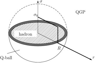
Figure 3: A schematic picture of the spherical Q-ball.

In the limit, we obtain the energy $E=\omega^{2}\sigma^{2}{\cal V}+V(\sigma^{2}){\cal V}$ and Q-charge $Q=2\omega\sigma^{2}{\cal V}$ with ${\cal V}$ being the volume of Q-ball, ${\cal V}=4\pi R^{3}/3$. A stable solution with fixed Q-charge is given by minimizing $E$ with respect to three variables $(\sigma,\omega,{\cal V})$ with the constraint $Q$ fixed. First, $E$ is expressed in terms of $(\sigma,{\cal V})$ as $E={1\over 4}{Q^{2}\over\sigma^{2}{\cal V}}+V(\sigma^{2}){\cal V}$. Then by minimizing it with respect to ${\cal V}$ one gets $E=Q\sqrt{\frac{V}{\sigma^{2}}}$ and ${\cal V}=\frac{Q}{\sqrt{4\sigma^{2}V}}$, which also determines $\omega$ in terms of $\sigma$ as $\omega^{2}\sigma^{2}=V(\sigma^{2})$. Finally, we determine the value of $\sigma$ by minimizing $E$ with respect to $\sigma$. Let $\sigma_{0}\neq 0$ be the value of $\sigma$ for which $E$ takes its minimum $E_{0}$, and $\omega_{0}$ be the corresponding frequency. Then, in summary, these values are determined by

$$E_{0}=Q\omega_{0},\qquad\omega_{0}^{2}=V^{\prime}(\sigma_{0}^{2}),\qquad\omega_{0}^{2}\sigma_{0}^{2}=V(\sigma_{0}^{2}),$$ (9)

where the prime stands for $V^{\prime}(\sigma^{2})=\partial V(\sigma^{2})/\partial(\sigma^{2})$. The last two equations determine both $\sigma_{0}$ and $\omega_{0}$ independently from $Q$. In fact these equations mean that the two extremal values of $U(\sigma)=V(\sigma^{2})-\omega_{0}^{2}\sigma^{2}$ coincide and $\sigma_{0}$ is one of the extrema with $\sigma_{0}\neq 0$, see Fig. 2. In this case, since $\sigma(r)$ can spend arbitrary long “time” $r$ at the extremum $\sigma=\sigma_{0}$, the solution can have an arbitrary large volume $\cal V$, and hence also the large Q-charge. Also, since the damping force in (7) is negligible after the long time, the profile $\sigma(r)$ is well approximated by the smoothed-out step function.

With the $Q$-ball at hand, we now see from Eq. (4) that the electric current arises along a constant background magnetic field $\vec{B}$ (the electric field is assumed to be zero)

$$\vec{\cal J}=\frac{3e^{2}}{4\pi^{2}}q^{2}\omega\vec{B}.$$ (10)

Here, we see that CME is a consequence of the existence of the Q-ball. The magnitude of our CME current is given dynamically by $\omega$ of the Q-ball. As found in (9), $\omega_{0}$ is given by the LSM potential characterized typically by $\Lambda_{\rm QCD}$. So it is natural to assume $\omega_{0}\sim\Lambda_{\rm QCD}$. Using the expected value of the magnetic field $eB\sim 10^{4}$ [MeV²] in heavy ion collisions Kharzeev:2007jp , we obtain the magnitude of the CME current as $|\vec{J}|\sim 10^{5}$ [MeV³] $\sim 10^{-2}$ [fm^-3].

Also, natural size of the Q-ball is $\sim Q^{1/3}{\rm[fm]}$, if all the dimensionful parameters are of order $\Lambda_{\rm QCD}\sim 1[{\rm fm}^{-1}]$.

Note that this important frequency $\omega$ plays a role of the so-called chiral chemical potential $\mu_{5}$ Fukushima:2008xe . The chemical potential can be introduced through the change $\partial_{0}\Phi\to(\partial_{0}+i\mu_{5})\Phi$ in ( Chiral Magnetic Effect from Q-balls). The relevant terms for this change are the ones with time derivatives:

$$|\partial_{0}\Phi|^{2}-\partial_{0}{\rm Im}(\log\Phi){3e^{2}q^{2}\over 8\pi^{2}}\vec{A}\cdot\vec{B}$$

$$\to|(\partial_{0}\!+\!i\mu_{5})\Phi|^{2}-\big{(}\partial_{0}{\rm Im}(\log\Phi)\!+\!\mu_{5}\big{)}{3e^{2}q^{2}\over 8\pi^{2}}\vec{A}\cdot\vec{B}.\qquad$$ (11)

Taking the Q-ball solution $\Phi=\sigma(r)e^{i\omega t}$ in the theory without $\mu_{5}$ is equivalent to considering a static solution $\Phi=\sigma(r)$ in the theory with $\mu_{5}$, if we identify $\mu_{5}=\omega$. In the latter case, the current (10) is supplied by the last $\mu_{5}\vec{A}\cdot\vec{B}$ term in (11).

Since the $Q$-charge is preserved, this non-topological soliton is fairly stable. However, the $h(\Phi+\Phi^{*})$ term in Eq. ( Chiral Magnetic Effect from Q-balls) breaking explicitly $U(1)_{\rm A}$ may destabilize the Q-ball, which would result in destroying a constant supply of the electric current. So, let us next analyze the effect of $h(\Phi+\Phi^{*})$. We expect that, if $h$ is sufficiently small, $U(1)_{\rm A}$ is broken only weakly and Q-ball still lives long. In the following, we shall derive a condition for $h$ to have the stability, and find that Q-ball are fairly stable, but with a new interesting feature of alternating CME current component.

We treat $h$ as a small parameter and we expand fields with respect to a small dimensionless parameter $\epsilon$ as

$$\Phi=\Phi_{0}+\epsilon\Phi_{1}+\epsilon^{2}\Phi_{2}+\cdots,\qquad\epsilon=\frac{h}{\sigma_{0}\omega_{0}^{2}},$$ (12)

where $\Phi_{0}$ is the $Q$-ball solution in $\epsilon\to 0$ limit. Again, we consider the large Q-ball limit given in Eq. (8). We would like to solve the equations of motion

$$F=\partial_{\mu}\partial^{\mu}\Phi+\Phi V^{\prime}-h=0,$$ (13)

order by order in $\epsilon$ as $F=F_{0}+\epsilon F_{1}+\epsilon^{2}F_{2}+\cdots=0$. The zeroth order $F_{0}=0$ is the Q-ball equation which we have solved. As we have seen, this gives us $\omega_{0}^{2}=V^{\prime}(\sigma_{0}^{2})$. The next-to-leading order is $F_{1}=0$ with $F_{1}$ given by

$$\partial_{\mu}\partial^{\mu}\Phi_{1}\!+\!\Phi_{1}\!V^{\prime}(|\Phi_{0}|^{2})\!+\!\Phi_{0}\!\left(\Phi_{0}^{*}\Phi_{1}\!+\!\Phi_{0}\Phi_{1}^{*}\right)\!V^{\prime\prime}(|\Phi_{0}|^{2})\!-\!\sigma_{0}\omega_{0}^{2}.$$

We solve this equation in two region, $r<R$ and $r>R$, separately. In the former region we put $\Phi_{0}=\sigma_{0}e^{i\omega_{0}t}$ while $\Phi_{0}=0$ in the latter region. Therefore, the next-to-leading order solution is given by

$$\Phi_{1}\big{|}_{r<R} = \frac{3\alpha_{1}-1}{3\alpha_{1}+2}\sigma_{0}+\frac{1}{3\alpha_{1}+2}\sigma_{0}e^{2i\omega_{0}t},$$ (14)

and $\Phi_{1}\big{|}_{r>R}=\sigma_{0}\omega_{0}^{2}/V^{\prime}(0)$, with $\alpha_{1}\equiv\frac{V^{\prime}(\sigma_{0}^{2})}{V^{\prime\prime}(\sigma_{0}^{2})\sigma_{0}^{2}}$. The next-to-next-to-leading order is readiliy solved by

$$\Phi_{2}\big{|}_{r<R}=\frac{-36\left(2+\alpha_{2}^{-1}\right)\alpha_{1}^{2}+9\alpha_{1}+2}{8\left(3\alpha_{1}+2\right)^{2}}\sigma_{0}e^{-i\omega_{0}t}$$

$$-\frac{9(2\!+\!\alpha_{2}^{-1})\alpha_{1}^{2}\!-\!6\alpha_{1}\!+\!2}{2(3\alpha_{1}+2)^{2}}\sigma_{0}e^{i\omega_{0}t}\!+\!\frac{3(-3\alpha_{1}\!+\!2)}{8(3\alpha_{1}+2)^{2}}\sigma_{0}e^{3i\omega_{0}t},$$

and $\Phi_{2}\big{|}_{r>R}=0$, where we have defined $\alpha_{2}=\frac{V^{\prime\prime}(\sigma_{0}^{2})}{V^{\prime\prime\prime}(\sigma_{0}^{2})\sigma_{0}^{2}}$. The mass of the Q-ball up to this order is evaluated as

$$E=Q\omega_{0}\!+\!{1\over 2}\left[\frac{3\left(-3(5\!+\!2\alpha^{-1}_{2})\alpha_{1}^{2}\!+\!3\alpha_{1}\!+\!2\right)}{(3\alpha_{1}+2)^{2}}+{\omega_{0}^{2}\over\mu^{2}}\right]Q\omega_{0}\epsilon^{2}$$

where we have shifted the origin of the energy in such a way that the energy density outside the Q-ball becomes zero, and $Q=2\omega_{0}\sigma_{0}^{2}{\cal V}$ as before. Note that the first contribution starts at the order of $\epsilon^{2}$ and the next is of order $\epsilon^{4}$. Therefore, the variation in energy is negligible if $\epsilon$ is sufficiently small, namely $h\ll\sigma_{0}\omega_{0}^{2}$. By using $\omega_{0}^{2}\sigma_{0}^{2}=V(\sigma_{0}^{2})$ (see (9)), this condition can be rewritten as $h\sigma_{0}\ll V(\sigma_{0}^{2})$. This condition is quite natural since it just means that the perturbation $h(\Phi+\Phi^{\ast})$ is small compared to the original potential $V(|\Phi|^{2})$. Hence we can expect that the Q-ball is stable against the perturbation.

Interestingly, a contribution of order $\epsilon$ arises in the electric current as

$$\vec{\cal J}=\frac{3e^{2}}{4\pi^{2}}q^{2}\vec{B}\omega_{0}\left(1-\epsilon\frac{3\alpha_{1}\!-\!2}{3\alpha_{1}\!+\!2}\cos\omega_{0}t+\cdots\right).$$ (15)

Thus the quark mass term and the $U(1)_{\rm A}$ anomaly in QCD eventually give rise to a small alternating CME current. This is a new feature of CME by the Q-ball.

Let us finally make a comment on a possibility of the Q-balls by the other pseudo-scalar mesons such as $\pi^{0}$ and $\eta$. In addition to $U(1)_{\rm A}$, there exists an axial part of the chiral symmetry $SU(3)_{\rm L-R}\in SU(3)_{\rm L}\times SU(3)_{\rm R}$ in QCD. It is straightforward to construct the Q-balls by using a $U(1)^{2}_{{\rm L}-{\rm R}}$ subgroup in $SU(3)_{\rm L-R}$, for instance, a pionic Q-ball with the $T^{3}$ generator. Since the $U(1)_{\rm L-R}^{2}$ is also anomalous by the electromagnetic interaction, the CME current arises as in the case of the $\eta^{\prime}$-ball .

In summary, we present a useful formalism of LSM which can explain CME in QGP via the non-topological soliton, Q-balls. The electric current arises along the external magnetic field and it has a small alternating current as a consequence of quark mass terms and the $U(1)_{\rm A}$ anomaly in addition. Furthermore, the interior of the Q-ball is the hadronic phase. So we predict that there may be a lump of hadrons, Q-ball, in QGP. It might have a certain contribution in the cooling process of QGP and hadronization.

In cosmology, the Q-ball is thought of as a candidate of so-called boson stars Jetzer:1991jr . We hope that our study may open a new direction to create baby boson stars at RHIC, LHC and FAIR.

Acknowledgment: The authors would like to thank Koichi Yazaki, Kenji Fukushima and Naoki Yamamoto for useful comments and discussions. The authors thank the Yukawa Institute for Theoretical Physics at Kyoto University. Discussions during the YITP workshops YITP-W-10-02 and YITP-W-10-08 were useful to complete this work. The work of M.E. and A.M. is supported by Special Postdoctoral Researchers Program at RIKEN. K.H. is partly supported by the Japan Ministry of Education, Culture, Sports, Science and Technology.

References

• (1) P. Huovinen, P. F. Kolb, U. W. Heinz, P. V. Ruuskanen and S. A. Voloshin, Phys. Lett.  B 503, 58 (2001).
• (2) S. S. Adler et al. [PHENIX Collaboration], Phys. Rev. Lett.  91, 182301 (2003).
• (3) J. Adams et al. [STAR Collaboration], Phys. Rev. Lett.  92, 052302 (2004).
• (4) D. E. Kharzeev, L. D. McLerran and H. J. Warringa, Nucl. Phys.  A 803, 227 (2008).
• (5) K. Fukushima, D. E. Kharzeev and H. J. Warringa, Phys. Rev.  D 78, 074033 (2008).
• (6) S. A. Voloshin [STAR Collaboration], Nucl. Phys.  A 830, 377C (2009).
• (7) K. Fukushima, M. Ruggieri and R. Gatto, Phys. Rev.  D 81, 114031 (2010).
• (8) A. Rebhan, A. Schmitt and S. A. Stricker, JHEP 1001, 026 (2010).
• (9) P. V. Buividovich, M. N. Chernodub, E. V. Luschevskaya and M. I. Polikarpov, Phys. Rev.  D 80, 054503 (2009).
• (10) S. R. Coleman, Nucl. Phys.  B 262, 263 (1985) [Erratum-ibid.  B 269, 744 (1986)].
• (11) D. T. Son and A. R. Zhitnitsky, Phys. Rev.  D 70, 074018 (2004).
• (12) D. E. Kharzeev, Annals Phys.  325, 205 (2010).
• (13) A. Gorsky and M. B. Voloshin, Phys. Rev.  D 82, 086008 (2010).
• (14) C. A. Baker et al., Phys. Rev. Lett.  97, 131801 (2006).
• (15) For a review, P. Jetzer, Phys. Rept.  220, 163-227 (1992).