Exact dynamical and partial symmetries

Abstract

We discuss a hierarchy of broken symmetries with special emphasis on partial dynamical symmetries (PDS). The latter correspond to a situation in which a non-invariant Hamiltonian accommodates a subset of solvable eigenstates with good symmetry, while other eigenstates are mixed. We present an algorithm for constructing Hamiltonians with this property and demonstrate the relevance of the PDS notion to nuclear spectroscopy, to quantum phase transitions and to mixed systems with coexisting regularity and chaos.

1 Introduction

Symmetries play an important role in dynamical systems. They provide quantum numbers for the classification of states, determine spectral degeneracies and selection rules, and facilitate the calculation of matrix elements. An exact symmetry occurs when the Hamiltonian of the system commutes with all the generators ($g_{i}$) of the symmetry-group $G$, $[\,\hat{H}\,,\,g_{i}\,]=0$. In this case, all states have good symmetry and are labeled by the irreducible representations (irreps) of $G$. The Hamiltonian admits a block structure so that inequivalent irreps do not mix and all eigenstates in the same irrep are degenerate. In a dynamical symmetry the Hamiltonian commutes with the Casimir operator of $G$, $[\,\hat{H}\,,\,\hat{C}_{G}\,]=0$, the block structure of $\hat{H}$ is retained, the states preserve the good symmetry but, in general, are no longer degenerate. When the symmetry is completely broken then $[\,\hat{H}\,,\,g_{i}\,]\neq 0$, and none of the states have good symmetry. In-between these limiting cases there may exist intermediate symmetry structures, called partial (dynamical) symmetries, for which the symmetry is neither exact nor completely broken. This novel concept of symmetry and its implications for dynamical systems are the focus of the present contribution.

Models based on spectrum generating algebras form a convenient framework to examine different types of symmetries and have been used extensively in diverse areas of physics [1, 2, 3]. In such models the Hamiltonian is expanded in elements of a Lie algebra, ($G_{0}$), called the spectrum generating algebra. A dynamical symmetry occurs if the Hamiltonian can be written in terms of the Casimir operators of a chain of nested algebras, $G_{0}\supset G_{1}\supset\ldots\supset G_{n}$. The following properties are then observed. (i) All states are solvable and analytic expressions are available for energies and other observables. (ii) All states are classified by quantum numbers, $|\alpha_{0},\alpha_{1},\ldots,\alpha_{n}\rangle$, which are the labels of the irreps of the algebras in the chain. (iii) The structure of wave functions is completely dictated by symmetry and is independent of the Hamiltonian’s parameters.

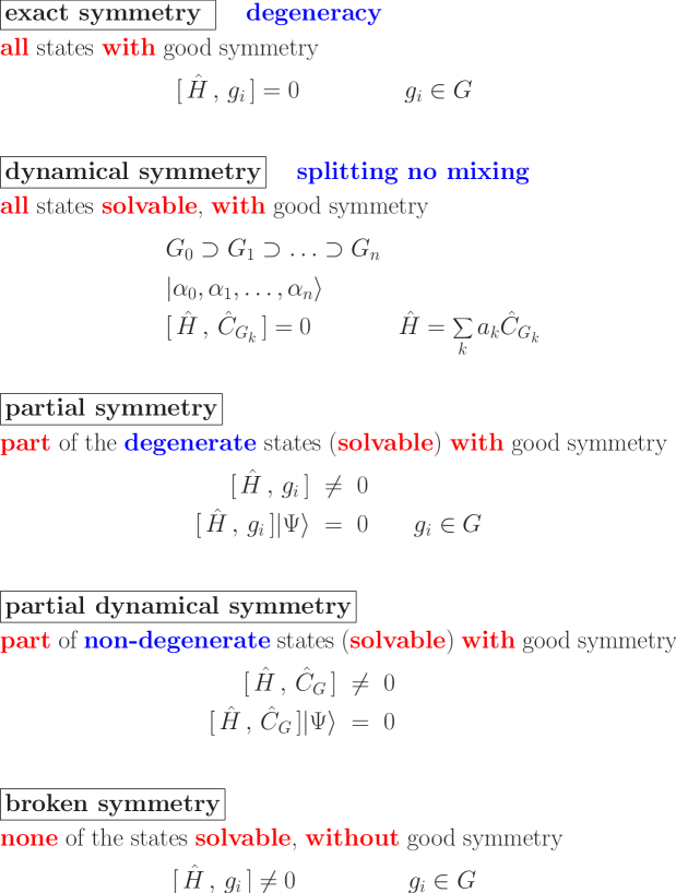
Figure 1: Hierarchy of symmetries.

The merits of a dynamical symmetry are self-evident. However, in most applications to realistic systems, the predictions of an exact dynamical symmetry are rarely fulfilled and one is compelled to break it. More often one finds that the assumed symmetry is not obeyed uniformly, i.e., is fulfilled by only some states but not by others. The required symmetry-breaking is achieved by including in the Hamiltonian terms associated with different sub-algebra chains of the parent spectrum generating algebra. In general, under such circumstances, solvability is lost, there are no remaining non-trivial conserved quantum numbers and all eigenstates are expected to be mixed. A partial dynamical symmetry (PDS) corresponds to a particular symmetry breaking for which some (but not all) of the virtues of a dynamical symmetry are retained. The essential idea is to relax the stringent conditions of complete solvability so that the properties (i)–(iii) are only partially satisfied [4].

The notion of partial dynamical symmetry generalizes the concepts of exact and dynamical symmetries. In making the transition from an exact to a dynamical symmetry, states which are degenerate in the former scheme are split but not mixed in the latter, and the block structure of the Hamiltonian is retained. Proceeding further to partial symmetry, some blocks or selected states in a block remain pure, while other states mix and lose the symmetry character. A partial dynamical symmetry lifts the remaining degeneracies, but preserves the symmetry-purity of the selected states. The hierarchy of broken symmetries is depicted in Fig. 1.

The existence of Hamiltonians with partial symmetry or partial dynamical symmetry is by no means obvious. An Hamiltonian with the above property is not invariant under the group $G$ nor does it commute with the Casimir invariants of $G$, so that various irreps are in general mixed in its eigenstates. However, it posses a subset of solvable states, denoted by $|\Psi\rangle$ in Fig. 1, which respect the symmetry. The commutator $[\,\hat{H}\,,\,g_{i}\,]$ or $[\,\hat{H}\,,\,\hat{C}_{G}\,]$ vanishes only when it acts on these ‘special’ states with good $G$-symmetry.

2 Partial dynamical symmetries

When a partial dynamical symmetry (PDS) occurs, the defining properties of a dynamical symmetry (DS), namely, solvability, good quantum numbers, and symmetry-dictated structure are fulfilled exactly, but by only a subset of states. An algorithm for constructing Hamiltonians with PDS has been developed in [5] and further elaborated in [6]. The analysis starts from the chain of nested algebras

$$\begin{array}[]{ccccccc}G_{\rm dyn}&\supset&G&\supset&\cdots&\supset&G_{\rm sym}\\ \downarrow&&\downarrow&&&&\downarrow\\[0.0pt] [h]&&\langle\Sigma\rangle&&&&\Lambda\end{array}$$ (1)

where, below each algebra, its associated labels of irreps are given. Eq. (1) implies that $G_{\rm dyn}$ is the dynamical (spectrum generating) algebra of the system such that operators of all physical observables can be written in terms of its generators; a single irrep of $G_{\rm dyn}$ contains all states of relevance in the problem. In contrast, $G_{\rm sym}$ is the symmetry algebra and a single of its irreps contains states that are degenerate in energy. Assuming, for simplicity, that particle number is conserved, then all states, and hence the representation $[h]$, can then be assigned a definite particle number $N$. For $N$ identical particles the representation $[h]$ of the dynamical algebra $G_{\rm dyn}$ is either symmetric $[N]$ (bosons) or antisymmetric $[1^{N}]$ (fermions) and will be denoted, in both cases, as $[h_{N}]$. The occurrence of a DS of the type (1) signifies that the Hamiltonian is written in terms of the Casimir operators of the algebras in the chain, $\hat{H}_{DS}=\sum_{G}a_{G}\,\hat{C}_{G}$, and the eigenstates can be labeled as $|[h_{N}]\langle\Sigma\rangle\dots\Lambda\rangle$; additional labels (indicated by $\dots$) are suppressed in the following. The eigenvalues of the Casimir operators in these basis states determine the eigenenergies $E_{DS}([h_{N}]\langle\Sigma\rangle\Lambda)$ of $\hat{H}_{DS}$. Likewise, operators can be classified according to their tensor character under (1) as $\hat{T}_{[h_{n}]\langle\sigma\rangle\lambda}$.

Of specific interest in the construction of a PDS associated with the reduction (1), are the $n$-particle annihilation operators $\hat{T}$ which satisfy the property

$$\hat{T}_{[h_{n}]\langle\sigma\rangle\lambda}|[h_{N}]\langle\Sigma_{0}\rangle\Lambda\rangle=0~{},$$ (2)

for all possible values of $\Lambda$ contained in a given irrep $\langle\Sigma_{0}\rangle$ of $G$. Equivalently, this condition can be phrased in terms of the action on a lowest weight (LW) state of the G-irrep $\langle\Sigma_{0}\rangle$, $\hat{T}_{[h_{n}]\langle\sigma\rangle\lambda}|LW;\,[h_{N}]\langle\Sigma_{0}\rangle\rangle=0$, from which states of good $\Lambda$ can be obtained by projection. Any $n$-body, number-conserving normal-ordered interaction written in terms of these annihilation operators and their Hermitian conjugates (which transform as the corresponding conjugate irreps), $\hat{H}=\sum_{\alpha,\beta}A_{\alpha\beta}\,\hat{T}^{{\dagger}}_{\alpha}\hat{T}_{\beta}$, has a partial G-symmetry. This comes about since for arbitrary coefficients, $A_{\alpha\beta}$, $\hat{H}$ is not a G-scalar, hence most of its eigenstates will be a mixture of irreps of G, yet relation (2) ensures that a subset of its eigenstates $|[h_{N}]\langle\Sigma_{0}\rangle\Lambda\rangle$, are solvable and have good quantum numbers under the chain (1). An Hamiltonian with partial dynamical symmetry is obtained by adding to $\hat{H}$ the dynamical symmetry Hamiltonian, $\hat{H}_{PDS}=\hat{H}_{DS}+\hat{H}$, still preserving the solvability of states with $\langle\Sigma\rangle=\langle\Sigma_{0}\rangle$.

If the operators $\hat{T}_{[h_{n}]\langle\sigma\rangle\lambda}$ span the entire irrep $\langle\sigma\rangle$ of G, then the annihilation condition (2) is satisfied for all $\Lambda$-states in $\langle\Sigma_{0}\rangle$, if none of the $G$ irreps $\langle\Sigma\rangle$ contained in the $G_{\rm dyn}$ irrep $[h_{N-n}]$ belongs to the $G$ Kronecker product $\langle\sigma\rangle\times\langle\Sigma_{0}\rangle$. So the problem of finding interactions that preserve solvability for part of the states (1) is reduced to carrying out a Kronecker product. If relation (2) holds only for some states $\Lambda$ in the irrep $\langle\Sigma_{0}\rangle$ and/or some components $\lambda$ of the tensor $\hat{T}_{[h_{n}]\langle\sigma\rangle\lambda}$, then the Kronecker product rule does not apply. However, the PDS Hamiltonian is still of the indicated normal-ordered form, but now the solvable states span only part of the corresponding $G$-irrep. The arguments for choosing the special irrep $\langle\Sigma\rangle=\langle\Sigma_{0}\rangle$ in Eq. (2), which contains the solvable states, are based on physical grounds. A frequently encountered choice is the irrep which contains the ground state of the system.

In what follows we illustrate the above procedure and demonstrate the relevance of the PDS notion to dynamical systems. For that purpose, we employ the interacting boson model (IBM) [2], widely used in the description of low-lying collective states in nuclei in terms of $N$ interacting monopole $(s)$ and quadrupole $(d)$ bosons representing valence nucleon pairs. The dynamical algebra is $G_{\rm dyn}={\rm U}(6)$ and the symmetry algebra is $G_{\rm sym}={\rm O}(3)$. The Hamiltonian commutes with the total number operator of $s$- and $d$- bosons, $\hat{N}$, which is the linear Casimir of U(6). Three DS limits occur in the model with leading subalgebras U(5), SU(3), and O(6), corresponding to typical collective spectra observed in nuclei, vibrational, rotational, and $\gamma$-unstable, respectively. A geometric visualization of the model is obtained by an energy surface

$$E_{N}(\beta,\gamma) = \langle\beta,\gamma;N|\hat{H}|\beta,\gamma;N\rangle~{},$$ (3)

defined by the expectation value of the Hamiltonian in the coherent (intrinsic) state [7, 8]

$$|\beta,\gamma;N\rangle = (N!)^{-1/2}(b^{\dagger}_{c})^{N}\,|0\,\rangle~{},$$ (4a)

$$b^{\dagger}_{c} = (1+\beta^{2})^{-1/2}[\beta\cos\gamma d^{\dagger}_{0}+\beta\sin{\gamma}(d^{\dagger}_{2}+d^{\dagger}_{-2})/\sqrt{2}+s^{\dagger}]~{}.$$ (4b)

Here $(\beta,\gamma)$ are quadrupole shape parameters whose values, $(\beta_{0},\gamma_{0})$, at the global minimum of $E_{N}(\beta,\gamma)$ define the equilibrium shape for a given Hamiltonian. For a Hamiltonian with one- and two-body interactions, the shape can be spherical $(\beta=0)$ or deformed $(\beta>0)$ with $\gamma=0$ (prolate), $\gamma=\pi/3$ (oblate), or $\gamma$-independent. The equilibrium deformations associated with the DS limits are $\beta_{0}=0$ for U(5), $(\beta_{0}=\sqrt{2},\gamma_{0}=0)$ for SU(3) and $(\beta_{0}=1,\gamma_{0}\,{\rm arbitrary})$ for O(6).

3 PDS and nuclear spectroscopy

The SU(3) DS chain of the IBM and related quantum numbers are given by [2]

$$\begin{array}[]{ccccc}{\rm U}(6)&\supset&{\rm SU}(3)&\supset&{\rm O}(3)\\ \downarrow&&\downarrow&&\downarrow\\[0.0pt] [N]&&\left(\lambda,\mu\right)&K&L\end{array}~{},$$ (8)

where $K$ is a multiplicity label needed for complete classification in the $SU(3)\supset O(3)$ reduction. The spectrum of the SU(3) DS Hamiltonian resembles that of an axially-deformed rotovibrator and the corresponding eigenstates are arranged in SU(3) multiplets. The label $K$ corresponds geometrically to the projection of the angular momentum on the symmetry axis. In a given SU(3) irrep $(\lambda,\mu)$, each $K$-value is associated with a rotational band and states with the same angular momentum $L$, in different $K$-bands, are degenerate. The lowest SU(3) irrep is $(2N,0)$, which describes the ground band $g(K=0)$ of a prolate deformed nucleus. The first excited SU(3) irrep $(2N-4,2)$ contains degenerate $\beta(K=0)$ and $\gamma(K=2)$ bands. This $\beta$-$\gamma$ degeneracy is a characteristic feature of the SU(3) limit which, however, is not commonly observed. In most deformed nuclei the $\beta$ band lies above the $\gamma$ band. In the IBM framework, with at most two-body interactions, one is therefore compelled to break SU(3) in order to conform with the experimental data.

The construction of Hamiltonians with SU(3)-PDS is based on identification of $n$-boson operators which annihilate all states in a given SU(3) irrep $(\lambda,\mu)$, chosen here to be the ground band irrep $(2N,0)$. For that purpose, we consider the following two-boson SU(3) tensors, $B^{\dagger}_{[n](\lambda,\mu)K;Lm}$, with $n=2$, $(\lambda,\mu)=(0,2)$ and angular momentum $L=0,\,2$

$$B^{\dagger}_{[2](0,2)0;00} \propto P^{\dagger}_{0}=d^{\dagger}\cdot d^{\dagger}-2(s^{\dagger})^{2}~{},$$ (9a)

$$B^{\dagger}_{[2](0,2)0;2m} \propto P^{\dagger}_{2m}=2d^{\dagger}_{m}s^{\dagger}+\sqrt{7}\,(d^{\dagger}\,d^{\dagger})^{(2)}_{m}~{}.$$ (9b)

The corresponding Hermitian conjugate boson-pair annihilation operators, $P_{0}$ and $P_{2m}$, transform as $(2,0)$ under SU(3), and satisfy

$$P_{0}\,|[N](2N,0)K=0,L\rangle = 0~{},$$

$$P_{2m}\,|[N](2N,0)K=0,L\rangle = 0~{}.$$ (10)

The indicated $L$-states span the entire SU(3) irrep $(\lambda,\mu)=(2N,0)$. They can be obtained by angular momentum projection from the coherent state, $|\beta=\sqrt{2},\gamma=0;N\rangle$, of Eq. (4), which is the lowest-weight state of this irrep and serves as an intrinsic state for the SU(3) ground band. The relations in Eq. (10) follow from the fact that the action of the operators $P_{Lm}$ leads to a state with $N-2$ bosons in the U(6) irrep $[N-2]$, which does not contain the SU(3) irreps obtained from the product $(2,0)\times(2N,0)=(2N+2,0)\oplus(2N,1)\oplus(2N-2,2)$. In addition, $P_{0}$ satisfies

$$P_{0}\,|[N](2N-4k,2k)K=2k,LM\rangle = 0~{},$$ (11)

where for $k>0$ the indicated $L$-states span only part of the SU(3) irreps $(\lambda,\mu)=(2N-4k,2k)$ and form the rotational members of excited $\gamma^{k}(K=2k)$ bands.

Following the general algorithm, a two-body Hamiltonian with partial SU(3) symmetry can now be constructed as [5, 9]

$$\hat{H}(h_{0},h_{2}) = h_{0}\,P^{\dagger}_{0}P_{0}+h_{2}\,P^{\dagger}_{2}\cdot\tilde{P}_{2}~{},$$ (12)

where $\tilde{P}_{2m}=(-)^{m}P_{2,-m}$ and the dot denotes a scalar product. For $h_{2}=h_{0}$, the Hamiltonian is an SU(3) scalar, related to the quadratic Casimir operator of SU(3), for $h_{0}=-5h_{2}$ it transforms as a $(2,2)$ SU(3) tensor component and has the form

$$\hat{H}(h_{0},h_{2}) = h_{2}\left[-\hat{C}_{{\rm SU(3)}}+2\hat{N}(2\hat{N}+3)\right]+(h_{0}-h_{2})\,P^{\dagger}_{0}P_{0}~{}.\quad$$ (13)

The first term in Eq. (13) belongs to the SU(3) DS Hamiltonian. The $P^{{\dagger}}_{0}P_{0}$ term is not diagonal in the SU(3) chain, however, Eqs. (10)-(11) ensure that $\hat{H}(h_{0},h_{2})$ retains selected solvable states with good SU(3) symmetry. Specifically, the solvable states are members of the ground $g(K=0)$ and $\gamma^{k}(K=2k)$ bands with the following characteristics

$$\begin{array}[]{lll}|N,(2N,0)K=0,L\rangle&E=0&L=0,2,4,\ldots,2N\\[7.0pt] |N,(2N-4k,2k)K=2k,L\rangle&E=h_{2}\,6k\left(2N-2k+1\right)&L=K,K+1,\ldots,(2N-2k)~{}.\end{array}\;\;$$ (16)

Figure 2: Spectra of ¹⁶⁸Er ($N=16$). Experimental energies (EXP) are compared with IBM calculations in an exact SU(3) dynamical symmetry [SU(3)], in a broken SU(3) symmetry (WCD) and in a partial dynamical SU(3) symmetry (PDS). The latter employs the Hamiltonian of Eq. (12), $\hat{H}(h_{0},h_{2})+C\,\hat{C}_{{\rm O(3)}}$, with $h_{0}=8,\,h_{2}=4,\,C=13$ keV.

The remaining eigenstates of $\hat{H}(h_{0},h_{2})$ do not preserve the SU(3) symmetry and therefore get mixed. This situation corresponds precisely to that of partial SU(3) symmetry. An Hamiltonian $\hat{H}(h_{0},h_{2})$ which is not an SU(3) scalar has a subset of solvable eigenstates which continue to have good SU(3) symmetry. One can add the Casimir operator of O(3), $\hat{C}_{{\rm O(3)}}$, to $\hat{H}(h_{0},h_{2})$ and by doing so, convert the partial SU(3) symmetry into partial dynamical SU(3) symmetry. The additional rotational term contributes just an $L(L+1)$ splitting but does not affect the wave functions.

The empirical spectrum of ¹⁶⁸Er is shown in Fig. 2 and compared with SU(3)-DS, SU(3)-PDS and broken SU(3) calculations [9]. The SU(3)-PDS spectrum shows an improvement over the schematic, exact SU(3) dynamical symmetry description, since the $\beta$-$\gamma$ degeneracy is lifted. The quality of the calculated PDS spectrum is similar to that obtained in the broken-SU(3) calculation, however, in the former the ground $g(K=0_{1})$ and $\gamma(K=2_{1})$ bands remain solvable with good SU(3) symmetry, $(\lambda,\mu)=(2N,0)$ and $(2N-4,2)$ respectively. At the same time, the excited $K=0^{+}_{2}$ band involves about $13\%$ SU(3) admixtures into the dominant $(2N-4,2)$ irrep. Since the wave functions of the solvable states (16) are known, one can obtain analytic expressions for matrix elements of observables between them. In particular, the calculated B(E2) ratios for $\gamma\to g$ transitions lead to parameter-free predictions in excellent agreement with experiment [9], thus confirming the relevance of SU(3)-PDS to the spectroscopy of ¹⁶⁸Er.

4 PDS and quantum phase transitions

Quantum phase transitions (QPT) occur at zero temperature as a function of a coupling constant in the Hamiltonian. Such ground-state energy phase transitions are a pervasive phenomenon observed in many branches of physics, and are realized empirically in nuclei as transitions between different shapes. QPTs occur as a result of a competition between terms in the Hamiltonian with different symmetry character, which lead to considerable mixing in the eigenfunctions, especially at the critical-point where the structure changes most rapidly. An interesting question to address is whether there are any symmetries (or traces of) still present at the critical points of QPT. As shown below, unexpectedly, partial dynamical symmetries can survive at the critical point in spite of the strong mixing [10].

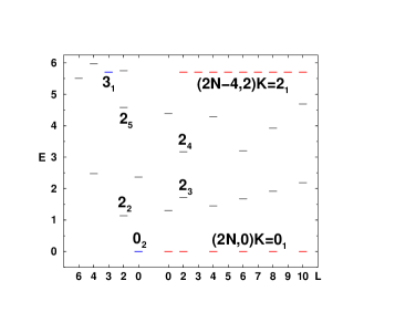
Figure 3: Spectrum of $\hat{H}_{cri}$, Eq. (18), with $h_{2}=0.05$ and $N=10$. $L(K=0_{1})$ and $L(K=2_{1})$ are the solvable SU(3) states of Eq. (16) with $k=0$ and $k=1$, respectively. $L=0_{2},3_{1}$ are the solvable U(5) states of Eq. (19).

Figure 4: U(5) ($n_{d}$) and SU(3) $[(\lambda,\mu)]$ decomposition for selected spherical and deformed states in Fig. 4.

A convenient framework to study symmetry aspects of QPTs in nuclei is the IBM  [2], whose dynamical symmetries correspond to possible phases of the system. The relevant Hamiltonian in such a study involves terms with from different DS chains. The nature of the phase transition is governed by the topology of the corresponding surface (3), which serves as a Landau’s potential with the equilibrium deformations as order parameters. The surface at the critical-point of a first-order transition is required to have two-degenerate minima, corresponding to the two coexisting phases. For example, the following first-order critical surface

$$E_{N}(\beta,\gamma=0) = 2h_{2}N(N-1)(1+\beta^{2})^{-2}\beta^{2}\left(\beta-\sqrt{2}\,\right)^{2}~{},$$ (17)

has degenerate spherical and deformed minima at $\beta=0$ and $(\beta=\sqrt{2},\gamma=0)$, corresponding to spherical and axially-deformed shapes. A barrier of height $h=2h_{2}N(N-1)(1-\sqrt{3}/2)$ separates the two minima. Such a surface can be obtained from Eq. (3) with the following Hamiltonian

$$\hat{H}_{cri} = h_{2}\,P^{\dagger}_{2}\cdot\tilde{P}_{2}~{},$$ (18)

which is qualified to be a critical Hamiltonian of a first-order transition between these shapes. $\hat{H}_{cri}$ is recognized to be a special case of the Hamiltonian of Eq. (12), shown to have SU(3)-PDS. As such, it has a subset of solvable eigenstates, Eq. (16), which are members of deformed ground $g(K=0)$ and $\gamma^{k}(K=2k)$ bands with good SU(3) symmetry, $(\lambda,\mu)=(2N-4k,2k)$. In addition, $H_{cri}$ has also the following solvable spherical eigenstates with good U(5) symmetry

$$|N,n_{d}=\tau=L=0\rangle\;\; E=0~{},$$ (19a)

$$|N,n_{d}=\tau=L=3\rangle\;\; E=6h_{2}(2N-1)~{}.\qquad\quad$$ (19b)

These are selected basis states, $|[N],n_{d},\tau,L\rangle$, of the U(5)-DS chain $U(6)\supset U(5)\supset O(5)\supset O(3)$. $H_{cri}$ (18) is not invariant under $U(5)$, nor does it have a U(5)-DS, yet it has solvable states with good U(5) symmetry. By definition, it posses a U(5)-PDS. The spherical $L=0$ state, Eq. (19a), is exactly degenerate with the SU(3) ground band, Eq. (16) with $k=0$, and the spherical $L=3$ state, Eq. (19b), is degenerate with the SU(3) $\gamma$-band, Eq. (16) with $k=1$. The remaining levels of $\hat{H}_{cri}$, shown in Fig. 4 are calculated numerically. Their wave functions are spread over many U(5) and SU(3) irreps, as is evident from the $n_{d}$ and $(\lambda,\mu)$ decomposition shown in Fig. 4. This situation, where some states are solvable with good U(5) symmetry, some are solvable with good SU(3) symmetry and all other states are mixed with respect to both U(5) and SU(3), defines a U(5) PDS coexisting with a SU(3) PDS. The presence in the spectrum of both spherical states (dominated by a single $n_{d}$ component) and deformed states arranged in bands (with a broad $n_{d}$ distribution) signals a first-order transition.

The above results demonstrate the relevance of the PDS notion to critical-points of QPT, with phases characterized by Lie-algebraic symmetries. In the example considered, first-order critical Hamiltonians exhibit distinct subsets of solvable states with good symmetries, giving rise to a coexistence of different PDS. The ingredients of an algebraic description of QPT is a spectrum generating algebra and an associated geometric space, formulated in terms of coherent (intrinsic) states. The same ingredients are used in the construction of Hamiltonians with PDS. These, in accord with the present discussion, can be used as tools to explore the role of partial symmetries in governing the critical behaviour of dynamical systems undergoing QPT.

5 PDS and mixed regular and chaotic dynamics

Partial dynamical symmetries can play a role not only for discrete spectroscopy but also for analyzing statistical aspects of nonintegrable systems. Hamiltonians with a dynamical symmetry are always completely integrable. The Casimir invariants of the algebras in the chain provide a set of constants of the motion in involution. The classical motion is purely regular. A symmetry-breaking is connected to nonintegrability and may give rise to chaotic motion. Hamiltonians with PDS are not completely integrable, hence can exhibit stochastic behavior, nor are they completely chaotic, since some eigenstates preserve the symmetry exactly. Consequently, such Hamiltonians are optimally suitable to the study of mixed systems with coexisting regularity and chaos.

The dynamics of a generic classical Hamiltonian system is mixed; KAM islands of regular motion and chaotic regions coexist in phase space. In the associated quantum system, if no separation between regular and irregular states is done, the statistical properties of the spectrum are usually intermediate between the Poisson and the Gaussian orthogonal ensemble (GOE) statistics. In a PDS, the symmetry of the subset of solvable states is exact, yet does not arise from invariance properties of the Hamiltonian. If the fraction of solvable states remains finite in the classical limit, one might expect that a corresponding fraction of the phase space would consist of KAM tori and exhibit regular motion. It turns out that PDS has an even greater effect on the dynamics. It is strongly correlated with suppression (i.e., reduction) of chaos even though the fraction of solvable states approaches zero in the classical limit [11, 12].

We consider the following IBM Hamiltonian

$$\hat{H}(\beta_{0}) = h_{0}\,P^{\dagger}_{0}(\beta_{0})P_{0}(\beta_{0})+h_{2}\,P^{\dagger}_{2}(\beta_{0})\cdot\tilde{P}_{2}(\beta_{0})~{},$$ (20)

where $P^{\dagger}_{0}(\beta_{0})=d^{\dagger}\cdot d^{\dagger}-\beta_{0}^{2}(s^{\dagger})^{2}$ and $P^{\dagger}_{2m}(\beta_{0})=\beta_{0}\sqrt{2}\,d^{\dagger}_{m}s^{\dagger}+\sqrt{7}\,(d^{\dagger}\,d^{\dagger})^{(2)}_{m}$. For $\beta_{0}=\sqrt{2}$, $\hat{H}(\beta_{0}=\sqrt{2})$ reduces to the Hamiltonian of Eq. (12), which has SU(3)-PDS with a subset of solvable states listed in Eq. (16). At a given spin per boson $l=L/N$, and to leading order in $1/N$, the fraction $f$ of solvable states decreases like $1/N^{2}$ with boson number. However, at a given boson number $N$, this fraction increases with $l$, a feature which is valid also for finite $N$ [11]. The classical Hamiltonian is obtained from (20) by replacing operators by c-numbers, $s^{{\dagger}},d^{{\dagger}}_{\mu}\to\alpha_{s}^{*},\alpha_{\mu}^{*}$ and taking $N\to\infty$, with $1/N$ playing the role of $\hbar$.

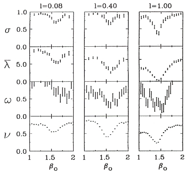
Figure 5: Classical $(\sigma,\bar{\lambda})$ and quantal $(\omega,\nu)$ measures of chaos versus $\beta_{0}$ for the Hamiltonian (20) with $h_{2}/h_{0}=7.5$. Shown are three cases with classical spins $l=0.08,\,0.4$, and $1$. The quantal calculations $(\omega,\nu)$ are done for $N=25$ bosons and spins $L=2,10$, and $25$, respectively. Notice that with increasing spin the minimum gets deeper and closer to $\beta_{0}=\sqrt{2}$. The suppression of chaos near $\beta_{0}=\sqrt{2}$ is seen both for finite $N$ through the measures $\omega,\,\nu$ and in the classical limit $N\to\infty$ through the measures $\sigma,\,\bar{\lambda}$.

To study the effect of the SU(3) PDS on the dynamics, we fix the ratio $h_{2}/h_{0}$ at a value far from the exact SU(3) symmetry (for which $h_{0}/h_{2}=1)$. We then change $\beta_{0}$ in the range $1\leq\beta_{0}\leq 2$. Classically, we determine the fraction $\sigma$ of chaotic volume and the average largest Lyapunov exponent $\bar{\lambda}$. To analyze the quantum Hamiltonian, we study spectral and transition intensity distributions. The nearest neighbors level spacing distribution is fitted by a Brody distribution, $P_{\omega}(S)=AS^{\omega}\exp(-\alpha S^{1+\omega})$, where $A$ and $\alpha$ are determined by the conditions that $P_{\omega}(S)$ is normalized to $1$ and $\langle S\rangle=1$. For the Poisson statistics $\omega=0$ and for GOE $\omega=1$, corresponding to integrable and fully chaotic classical motion, respectively. The intensity distribution of the E2 operator is fitted by a $\chi^{2}$ distribution in $\nu$ degrees of freedom, $P_{\nu}(y)=[(\nu/2\langle y\rangle)^{\nu/2}/\Gamma(\nu/2)]y^{\nu/2-1}\exp(-\nu y/2\langle y\rangle)$. For the GOE, $\nu=1$ and $\nu$ decreases as the dynamics become more regular.

Fig. 5 shows the two classical measures $\sigma$, $\bar{\lambda}$ and the two quantum measures $\omega$, $\nu$ for the Hamiltonian (20) as a function of $\beta_{0}$. The parameters of the Hamiltonian are taken to be $h_{2}/h_{0}=7.5$ and the number of bosons is $N=25$. Shown are three classical spins $l=0.08,\,0.4$ and $1$, which correspond in the quantum case to $L=2,\,10$ and $25$. All measures show a pronounced minimum which gets deeper and closer to $\beta_{0}=\sqrt{2}$ [where the partial SU(3) symmetry occurs] as the classical spin increases. This behaviour is correlated with the fraction of solvable states (at a constant $N$) being larger at higher $l$. We remark that the classical measures show a clear enhancement of the regular motion near $\beta_{0}=\sqrt{2}$ even though the fraction of solvable states vanishes as $1/N^{2}$ in the classical limit $N\to\infty$. That the observed suppression of chaos is related to the SU(3) PDS, is confirmed by the fact that the SU(3) entropy averaged over all eigenstates of $\hat{H}(\beta_{0})$ displays a minimum which is well correlated with the minimum in Fig. 5. The existence of an SU(3) PDS seems to have an effect of increasing the SU(3) symmetry of all states, not just those with an exact SU(3) symmetry.

The following physical picture emerges from the analysis of low-dimensional systems [11, 12]. At the quantum level, PDS by definition implies the existence of a “special” subset of states, which observe the symmetry. The PDS affects the purity of other states in the system; in particular, neighboring states, accessible by perturbation theory, possess approximately good symmetry. Analogously, at the classical level, the region of phase space near the “special” torus also has toroidal structure. As a consequence of having PDS, a finite region of phase space is regular and a finite fraction of states is approximately “special”. This clarifies the observed suppression of chaos.

6 Concluding remarks

Underlying the PDS notion, is the recognition that a non-invariant Hamiltonian can have selected eigenstates with good symmetry and good quantum numbers. In such a case, the symmetry in question is preserved in some states but is broken in the Hamiltonian (an opposite situation to that encountered in a spontaneously-broken symmetry). PDSs appear to be a common feature in algebraic descriptions of dynamical systems. They are not restricted to a specific model but can be applied to any quantal systems of interacting particles, bosons and fermions [4, 13, 14].

In PDS of type I described above, only part of the eigenspectrum is analytically solvable and retains all the dynamical symmetry (DS) quantum numbers. Additional types of PDS are possible. In PDS of type II, the entire eigenspectrum retains some of the DS quantum numbers [15]. PDS of type III has a hybrid character, in the sense that some (solvable) eigenstates keep some of the quantum numbers [16]. General algorithms for selecting and constructing Hamiltonians with PDSs of various types are available. The advantage of using interactions with a PDS is that they can be introduced, in a controlled manner, without destroying results previously obtained with a DS for a segment of the spectrum. These virtues generate an efficient tool which greatly enhance the scope of applications of algebraic modeling of quantum many-body systems. This work is supported by the Israel Science Foundation and the BSF.

References

- [1] Bohm A, Néeman Y and Barut A O eds 1988 Dynamical Groups and Spectrum Generating Algebras (Singapore: World Scientific)
- [2] Iachello F and Arima A 1987 The Interacting Boson Model (Cambridge: Cambridge Univ. Press)
- [3] Iachello F and Levine R D 1994 Algebraic Theory of Molecules (Oxford: Oxford Univ. Press)
- [4] Leviatan A 2011 Prog. Part. Nucl. Phys. 66 93
- [5] Alhassid Y and Leviatan A 1992 J. Phys. A 25 L1265
- [6] García-Ramos J E, Leviatan A and Van Isacker P 2009 Phys. Rev. Lett. 102 112502
- [7] Ginocchio J N and Kirson M W 1980 Phys. Rev. Lett. 44 1744
- [8] Dieperink A E L, Scholten O and Iachello F 1980 Phys. Rev. Lett. 44 1747
- [9] Leviatan A 1996 Phys. Rev. Lett. 77 818
- [10] Leviatan A 2007 Phys. Rev. Lett. 98 242502
- [11] Whelan N , Alhassid Y and Leviatan A 1993 Phys. Rev. Lett. 71 2208
- [12] Leviatan A and Whelan N D 1996 Phys. Rev. Lett. 77 5202
- [13] Escher J and Leviatan A 2000 Phys. Rev. Lett. 84 1866
- [14] Van Isacker P and Heinze S 2008 Phys. Rev. Lett. 100 052501
- [15] Van Isacker P 1999 Phys. Rev. Lett. 83 4269
- [16] Leviatan A and Van Isacker P 2002 Phys. Rev. Lett. 89 222501