High order explicit symplectic integrators
for the Discrete Non Linear Schrödinger equation

by Jehan Boreux, Timoteo Carletti and Charles Hubaux Report naXys-09-2010                   12 December 2010

Namur Center for Complex Systems

University of Namur
8, rempart de la vierge, B5000 Namur (Belgium)
http://www.naxys.be

Abstract.

We propose a family of reliable symplectic integrators adapted to the Discrete Non–Linear Schrödinger equation; based on an idea of Yoshida [12] we can construct high order numerical schemes, that result to be explicit methods and thus very fast. The performances of the integrators are discussed, studied as functions of the integration time step and compared with some non symplectic methods.

1. Introduction

The one dimensional Nonlinear Schrödinger System (NLS) [6] :

(1) $$\begin{cases}\;\;i\partial_{t}q+\partial_{xx}q+2q^{2}p=0\\ -i\partial_{t}p+\partial_{xx}p+2p^{2}q=0\,,\end{cases}$$

under periodic boundary conditions, $\left(p(x+L,t),q(x+L,t)\right)=\left(p(x,t),q(x,t)\right)$ for all $x$ and $t$, is a widely studied multiparticles system subjected to nonlinear interactions, that can be used to model several relevant physical phenomena [9], ranging from optics to solid state and atomic physics, for instance Bose-Einstein condensates.

Often scientists, once modeling physical nonlinear phenomena, impose the condition  $\overline{p(t)}=\pm q(t)$ for all $t$, in this case the system reduces to the standard cubic NLS equation. We hereby adopt the viewpoint of [5] where the conjugacy relation between $p(t)$ and $q(t)$ is not imposed a priori. We will nevertheless show that if this relation holds at $t=0$ then it will be preserved by our numerical integration scheme.

Most properties of NLS are related to the asymptotic behavior of its solutions, there is thus a strong need for integration schemes, allowing large step sizes, to easily cover large time spans, without degrading the efficiency of the numerical method hence avoiding the introduction of spurious outcome in the numerical simulations. These goals can be achieved using symplectic integrators, that are specifically designed to preserve the energy and possibly other first integral of the system. Our analysis will be performed on the following one dimensional discretization of the Eq. (1), DNLS for short [5]:

(2) $$\forall l\in\{1,\dots,N\}\quad\begin{cases}\dot{p_{l}}&=-\frac{i}{h^{2}}\left(p_{l+1}-2p_{l}+p_{l-1}\right)-2ip_{l}^{2}q_{l}\\ \dot{q_{l}}&=\frac{i}{h^{2}}\left(q_{l+1}-2q_{l}+q_{l-1}\right)+2ip_{l}q_{l}^{2}\,,\end{cases}$$

using the periodic boundary conditions $q_{l+N}=q_{l}$ and $p_{l+N}=p_{l}$ for all $l\in\{1,\dots,N\}$. Let us observe that the solutions of the DNLS are $\mathcal{O}(h^{2})$ close to the solutions of the PDE (1), thus in the limit $h\rightarrow 0$, the former converge to the solutions of the latter.

The integration method hereby proposed is based on the development of an idea introduced by Yoshida [12]. The strong improvement allowed by this method with respect to other ones available in the literature, relies on the fact that we are able to provide symplectic integrators, that are explicit ones, thus very fast, and whose order can be easily as high as the eighth one. Other methods based on the construction of generating functions, see for instance [1, 7] are not particularly suitable because the Hamiltonian function describing the DNLS cannot be split in the form $H(p,q)=T(p)+V(q)$, namely it is not a potential Hamiltonian system. This implies in fact that the obtained numerical integration schemes are implicit methods, and thus a large amount of CPU time is used to compute the new position, or the new momentum, using some Newton–like method. Let us observe that Gauss’ methods [4], namely symplectic versions of Runge–Kutta, are also implicit ones and thus they suffer of the above mentioned limitations.

Finally let us observe that, because the system cannot be put in the form of a perturbation of an integrable system, the method proposed in [8] is no more useful here: one can easily get a second order method and with some additional work also a fourth order method [11], but no higher orders are obtainable.

The paper is organized as follows. In the next section we briefly recall the Hamiltonian structure of the non linear Schrödinger equation on a one dimensional lattice; then Section 3 will be devoted to the presentation and to the construction of the symplectic integrator, whose properties will be numerically studied in Section 4. Finally we sum up and draw our conclusions in Section 5.

2. The non linear Schrödinger equation on a lattice

The system (1) will be studied imposing the standard spatial discretization, see for instance [5], thereby called Diagonal NLS, that reads:

(3) $$\forall l\in\{1,\dots,N\}\quad\begin{cases}\dot{p_{l}}&=-\frac{i}{h^{2}}\left(p_{l+1}-2p_{l}+p_{l-1}\right)-2ip_{l}^{2}q_{l}\\ \dot{q_{l}}&=\frac{i}{h^{2}}\left(q_{l+1}-2q_{l}+q_{l-1}\right)+2ip_{l}q_{l}^{2}\,,\end{cases}$$

using the periodic boundary conditions:

(4) $$q_{l+N}=q_{l}\quad\text{and}\quad p_{l+N}=p_{l}\quad\forall l\in\{1,\dots,N\}\,.$$

Observe that $h$ plays the role of spatial discretization parameter and thus the first terms on the right hand sides stem from the discretized second order spatial derivatives.

Let us remark that one could be interested in studying directly the system (3) as a relevant model of non–linear interaction on a discrete one dimensional of lattice.

One can easily prove that the DNLS can be cast into the Hamiltonian formalism using the following Hamilton function

(5) $$H(\vec{p},\vec{q})=-i\sum_{l=1}^{N}\left[\frac{(p_{l+1}-p_{l})(q_{l+1}-q_{l})}{h^{2}}-p_{l}^{2}q_{l}^{2}\right]\,,$$

and moreover the variables $(p_{l},q_{l})\in\mathbb{C}^{n}$ do satisfy the standard Poisson equations

$$\{p_{l},p_{m}\}=\{q_{l},q_{m}\}=0\quad\text{and}\quad\{p_{l},q_{m}\}=\delta_{l,m}\quad\forall l,m\in\{1,\dots,N\}\,.$$

Remark 2.1.

Let us observe that the DNLS system (3) possesses another first integral independent of the energy, namely:

(6) $$I(\vec{p},\vec{q})=\sum_{l=1}^{N}p_{l}q_{l}\,,$$

that under the assumption $\overline{p(t)}=q(t)$, is usually called the mass of the system.

The aim of this work is to define a family of symplectic integrators based on the Yoshida symplectic scheme [12] adapted to the DNLS system (3) and to study their numerical properties in terms of preserved quantities, CPU time needed and accuracy of the results.

Let us observe that system (3) is not quasi–integrable, i.e. it cannot be decomposed as the sum of an integrable one and a “small perturbation”, thus we cannot use the high order symplectic schemes $SABA_{n}$ or $SBAB_{n}$ proposed by Laskar and Robutel [8], whose accuracy strongly relies on the smallness of the perturbation.

3. A symplectic scheme

For a sake of completeness, let us briefly recall the integration method proposed in [12] to numerically reconstruct the orbit of an Hamiltonian systems $H(\vec{p},\vec{q})$.

Given any initial condition $\left(\vec{p}(0),\vec{q}(0)\right)$ and an integration time span $[0,T]$, we proceed by decomposing the integration interval into small pieces of fixed size $\tau$. The method results thus in a fixed step size integration method. Then, in each small interval, we approximate the time $\tau$ flow of the Hamiltonian systems

$$\begin{cases}\dot{\vec{p}}&=-\frac{\partial H}{\partial\vec{q}}\\ \dot{\vec{q}}&=\frac{\partial H}{\partial\vec{p}}\,,\end{cases}$$

by a composition of basic symplectic flows of the form $\exp\left(\tau c_{j}L_{A}\right)$ and $\exp\left(\tau d_{j}L_{B}\right)$, where $A(\vec{p},\vec{q})$ and $B(\vec{p},\vec{q})$ are two suitable functions providing a decomposition of the Hamilton function, i.e. $H=A+B$, $(c_{j},d_{j})$ suitable constants to achieve the wanted order of precision of the integration scheme and $\exp\left(\tau L_{H}\right)$ is a shorthand notation to denote the flow at time $\tau$ of the Hamilton function $H$. More precisely we are looking for

(7) $$\exp\left(\tau L_{A+B}\right)=\exp\left(\tau c_{1}L_{A}\right)\circ\exp\left(\tau d_{1}L_{B}\right)\circ\dots\circ\exp\left(\tau c_{k}L_{A}\right)\circ\exp\left(\tau d_{k}L_{B}\right)+\mathcal{O}(\tau^{n})\,,$$

for some positive integers $k$ and $n$.

The method is particularly efficient once the maps $\exp\left(\tau c_{j}L_{A}\right)$ and $\exp\left(\tau d_{j}L_{B}\right)$ are explicitely computable, which requires $A$ and $B$ to be simple enough. In particular this is true whenever $A$ and $B$ depend only upon one group of canonical variables and thus the Hamiltonian is of the so-called potential form. Of course this is a strong requirement that cannot always be achieved by suitable change of coordinates. In the following we propose the decomposition of the Hamilton function (5) given by

(8) $$A(\vec{p},\vec{q})=i\sum_{l=1}^{N}p_{l}^{2}q_{l}^{2}\quad\text{and}\quad B(\vec{p},\vec{q})=-i\sum_{l=1}^{N}\frac{(p_{l+1}-p_{l})(q_{l+1}-q_{l})}{h^{2}}\,.$$

Let us observe that even if $A$ and $B$ both depend on all the canonical variables, we are able to explicitely compute $\exp\left(\tau L_{A}\right)$ and $\exp\left(\tau L_{B}\right)$ (see § 3.1 and § 3.2) and thus to propose a completely explicit method.

3.1. Computation of $\exp\left(\tau L_{A}\right)$

The equations of motion of the system with “Hamilton function”$A$ are given by:

(9) $$\forall l\in\{1,\dots,N\}\quad\begin{cases}\dot{p}_{l}&=-2ip_{l}^{2}q_{l}\\ \dot{q}_{l}&=2ip_{l}q^{2}_{l}\,,\end{cases}$$

from which it trivially follows that $p_{l}q_{l}=C_{l}$ is a first integral for all $l$, in fact:

$$\frac{d}{dt}C_{l}\rvert_{\text{flow~{}\eqref{eq:expA1}}}=\dot{p}_{l}q_{l}+p_{l}\dot{q}_{l}=-2ip_{l}^{2}q^{2}_{l}+2ip_{l}^{2}q^{2}_{l}=0\,.$$

Hence (9) simplifies into

(10) $$\forall l\in\{1,\dots,N\}\quad\begin{cases}\dot{p}_{l}&=-2ip_{l}C_{l}\\ \dot{q}_{l}&=2iq_{l}C_{l}\,,\end{cases}$$

whose solution with initial datum $(p_{l}(0),q_{l}(0))_{l=1,\dots,N}$ is for all $t$:

(11) $$\forall l\in\{1,\dots,N\}\quad\begin{cases}p_{l}(t)&=e^{-2iC_{l}t}p_{l}(0)\\ q_{l}(t)&=e^{2iC_{l}t}q_{l}(0)\,.\end{cases}$$

Finally the time $\tau$ flow of $A$ is given by:

(12) $$(\vec{p^{\prime}},\vec{q^{\prime}})^{\rm T} = e^{\tau L_{A}}(\vec{p},\vec{q})^{\rm T}=e^{\tau L_{A}}(p_{1},\dots,p_{N},q_{1},\dots,q_{N})^{\rm T}$$

$$= (e^{-2ip_{1}q_{1}\tau}p_{1},\dots,e^{-2ip_{N}q_{N}\tau}p_{N},e^{2ip_{1}q_{1}\tau}q_{1},\dots,e^{2ip_{N}q_{N}\tau}q_{N})^{\rm T}\,,$$

where ^T denotes the transposed of the vector.

3.2. Computation of $\exp\left(\tau L_{B}\right)$

The equations of motion corresponding to the $B$ part of the Hamiltonian function are:

(13) $$\forall l\in\{1,\dots,N\}\quad\begin{cases}\dot{p_{l}}&=-\frac{i}{h^{2}}\left(p_{l+1}-2p_{l}+p_{l-1}\right)\\ \dot{q_{l}}&=\frac{i}{h^{2}}\left(q_{l+1}-2q_{l}+q_{l-1}\right)\,,\end{cases}$$

that can be cast in a compact form using the periodic boundary conditions (4) by introducing the circulant matrix [2] $M$ obtained by cyclically permute the $N$–vector $(-2,1,0,\dots,0,1)$:

(14) $$M=\left(\begin{matrix}-2&1&0&\ldots&\ldots&0&1\\ 1&-2&1&0&\ldots&\ldots&0\\ 0&1&-2&1&0&\ldots&0\\ \vdots&\ddots&\ddots&\ddots&\ddots&&\vdots\\ \vdots&&\ddots&\ddots&\ddots&&\vdots\\ \vdots&&&\ddots&\ddots&\ddots&\vdots\\ 1&0&\ldots&\ldots&0&1&-2\end{matrix}\right)\,,$$

that is the linear diagonal system

(15) $$\begin{cases}\dot{\vec{p}}&=-\frac{i}{h^{2}}M\vec{p}\\ \dot{\vec{q}}&=\frac{i}{h^{2}}M\vec{q}\,.\end{cases}$$

Thus formally the time $\tau$ flow of the Hamilton function $B$ is given by:

(16) $$(\vec{p^{\prime}},\vec{q^{\prime}})^{\rm T} = e^{\tau L_{B}}(\vec{p},\vec{q})^{\rm T}=(e^{-\frac{i}{h^{2}}\tau M}\vec{p},e^{\frac{i}{h^{2}}\tau M}\vec{q})^{\rm T}\,.$$

The circulant matrices have some useful properties that allow one to explicitely compute their eigenvalues, eigenvectors and hence their exponential.

Proposition 3.1 (Circulant matrix).

Let $M$ be the circulant matrix given by (14) and let $\rho=e^{2\pi i/N}$, then

1. The eigenvalues of the matrix $M$ are given by: $\mu_{j}=-2+\rho^{j}+\rho^{j(N-1)}$, $j=0,\dots,N-1$;

2. For $j=0,\dots,N-1$, the eigenvector associated to $\mu_{j}$ is given by

   $$w_{j}=\frac{1}{\sqrt{N}}\left(1,\rho^{j},\rho^{2j},\dots,\rho^{j(N-1)}\right)^{\rm T}\,;$$

3. Let $W$ be the matrix whose columns are the eigenvectors $w_{0},\dots,w_{N-1}$, then $W$ is unitary, namely $WW^{{\dagger}}=W^{{\dagger}}W=1_{N}$. Where ^† denotes the transposed complex conjugated matrix;

4. The exponential of $M$ is given by:

   $$e^{M}=We^{M_{\text{diag}}}W^{{\dagger}}\Rightarrow\forall l,m\in\{1,\dots,N\}\quad(e^{M})_{lm}=\frac{1}{N}\sum_{k=1}^{N}e^{\mu_{k-1}}\rho^{(l-m)(k-1)}\,,$$

   being $M_{\text{diag}}$ the diagonal matrix with the eigenvalues on the diagonal.

Proof.

Point (1) can be proved by a direct computation, for all $j\in\{0,\dots,N-1\}$, one has:

$$Mw_{j}=\frac{1}{\sqrt{N}}M\left(\begin{smallmatrix}1\\ \rho^{j}\\ \vdots\\ \rho^{j(N-1)}\end{smallmatrix}\right)=\frac{1}{\sqrt{N}}\left(\begin{smallmatrix}-2+\rho^{j}+\rho^{j(N-1)}\\ 1-2\rho^{j}+\rho^{2j}\\ \vdots\\ 1+\rho^{j(N-2)}-2\rho^{j(N-1)}\end{smallmatrix}\right)=\frac{1}{\sqrt{N}}\left(\begin{smallmatrix}-2+\rho^{j}+\rho^{j(N-1)}\\ \rho^{j}(\rho^{-j}-2+\rho^{j})\\ \vdots\\ \rho^{j(N-1)}(\rho^{-j(N-1)}+\rho^{-j}-2)\end{smallmatrix}\right)\,,$$

observing that $\rho^{N}=1$, we thus have

$$Mw_{j}=\frac{-2+\rho^{j}+\rho^{j(N-1)}}{\sqrt{N}}\left(\begin{smallmatrix}1\\ \rho^{j}\\ \vdots\\ \rho^{j(N-1)}\end{smallmatrix}\right)=\mu_{j}w_{j}\,.$$

Let us point out that the complex vectors $(w_{j})_{j=0,\dots,N-1}$ form an orthonormal set for $\mathbb{C}^{N}$ (with the standard complex scalar product):

$$<w_{j},w_{k}>=\sum_{m=1}^{N}\overline{w}_{j,m}w_{k,m}=\frac{1}{N}\sum_{m=1}^{N}\rho^{-j(m-1)}\rho^{k(m-1)}=\frac{1}{N}\sum_{m=1}^{N}\rho^{-(j-k)(m-1)}=\delta_{jk}\,.$$

Let us also remark that the eigenvalues $\mu_{j}$ are actually real:

$$\mu_{j}=-2+\rho^{j}+\rho^{j(N-1)}=-2+\rho^{j}+\rho^{-j}=-2+2\cos(2\pi j/N)\,,$$

and moreover the eigenvalues coincide in pairs, more precisely there are $(N-1)/2$ distinct eigenvalues, if $N$ is odd, and $(N-2)/2$ ones if $N$ is even: $\mu_{j}=\mu_{k}$ if $(j+k)\mod N=0$.

To prove that $W$ is unitary, let us denote by $X=WW^{{\dagger}}$ and compute the element $j,k$ of such matrix. By definition

$$X_{jk}=\sum_{l=1}^{N}W_{jl}W_{lk}^{{\dagger}}=\sum_{l=1}^{N}W_{jl}\overline{W}_{kl}=\frac{1}{N}\sum_{l=1}^{N}\rho^{(j-1)(l-1)}\rho^{-(k-1)(l-1)}=\frac{1}{N}\sum_{l=1}^{N}\rho^{(j-k)(l-1)}=\delta_{jk}\,,$$

thus $X=1_{N}$. A similar computation can be done for $W^{{\dagger}}W$.

Finally let us observe that $MW=WM_{\text{diag}}$, in fact one trivially has

$$MW=(\mu_{0}w_{0}|\ldots|\mu_{N-1}w_{N-1})=WM_{\text{diag}}\,,$$

and because $W$ is unitary, $W^{-1}=W^{{\dagger}}$, thus $M=WM_{\text{diag}}W^{{\dagger}}$. This implies that the exponential can be computed as follows:

$$e^{M}=e^{WM_{\text{diag}}W^{{\dagger}}}=We^{M_{\text{diag}}}W^{{\dagger}}\,.$$

The element $l,m$ of $e^{M}$ is thus given by:

$$(e^{M})_{lm} = \sum_{k=1}^{N}W_{lk}e^{\mu_{k-1}}W_{km}^{{\dagger}}=\sum_{k=1}^{N}W_{lk}e^{\mu_{k-1}}\overline{W}_{mk}=\frac{1}{N}\sum_{k=1}^{N}e^{\mu_{k-1}}\rho^{(l-1)(k-1)}\rho^{-(m-1)(k-1)}$$

$$= \frac{1}{N}\sum_{k=1}^{N}e^{\mu_{k-1}}\rho^{(l-m)(k-1)}\,.$$

∎

One can thus explicitely compute the flow of $B$ given by (16)

Corollary 3.2.

The time $\tau$ flow of the Hamilton function $B$ can be rewritten as:

(17) $$\begin{cases}\vec{p^{\prime}}&=We^{-\frac{i}{h^{2}}\tau M_{\text{diag}}}W^{{\dagger}}\vec{p}\\ \vec{q^{\prime}}&=We^{\frac{i}{h^{2}}\tau M_{\text{diag}}}W^{{\dagger}}\vec{q}\,,\end{cases}$$

or explicitely for all $l\in\{1,\dots,N\}$:

(18) $$\begin{cases}p_{l}^{\prime}=\frac{1}{N}\sum_{m=1}^{N}\sum_{k=1}^{N}e^{-\frac{i}{h^{2}}\tau\mu_{k-1}}\rho^{(l-m)(k-1)}p_{m}\\ q_{l}^{\prime}=\frac{1}{N}\sum_{m=1}^{N}\sum_{k=1}^{N}e^{\frac{i}{h^{2}}\tau\mu_{k-1}}\rho^{(l-m)(k-1)}q_{m}\ .\end{cases}$$

Let us observe that (18) can be rewritten in compact vector form in a way inspired by the solution of linear ODE, namely as a linear combination of eigenvectors, as follows:

(19) $$\begin{cases}\vec{p^{\prime}}&=e^{-\frac{i}{h^{2}}\tau\mu_{0}}<w_{0},\vec{p}(0)>w_{0}+\dots+e^{-\frac{i}{h^{2}}\tau\mu_{N-1}}<w_{N-1},\vec{p}(0)>w_{N-1}\\ \vec{q^{\prime}}&=e^{\frac{i}{h^{2}}\tau\mu_{0}}<w_{0},\vec{q}(0)>w_{0}+\dots+e^{-\frac{i}{h^{2}}\tau\mu_{N-1}}<w_{N-1},\vec{q}(0)>w_{N-1}\,.\end{cases}$$

3.3. The integrator

Once we have the explicit maps $\exp\left(\tau L_{A}\right)$ and $\exp\left(\tau L_{B}\right)$ one can construct the basic second order symplectic scheme Störmer-Verlet/Leap Frog: $Y_{2}(\tau)=e^{\frac{\tau}{2}L_{A}}e^{\tau L_{B}}e^{\frac{\tau}{2}L_{A}}$. Then Yoshida proved [12] that one can find explicit suitable coefficients $x_{1}=\frac{1}{2-2^{1/3}}$ and $x_{0}=-2^{1/3}x_{1}$, such that the composition

(20) $$Y_{4}(\tau)=Y_{2}\left(x_{1}\tau\right)\circ Y_{2}\left(x_{0}\tau\right)\circ Y_{2}\left(x_{1}\tau\right)\,,$$

is actually a fourth order symplectic integrator, that moreover is symmetric, i.e. it has exact time reversibility.

One can iterate this construction and find new explicit coefficients, $y_{1}=\frac{1}{2-2^{1/5}}$ and $y_{0}=-2^{1/5}y_{1}$, such that the composition

(21) $$Y_{6}(\tau)=Y_{4}\left(y_{1}\tau\right)\circ Y_{4}\left(y_{0}\tau\right)\circ Y_{4}\left(y_{1}\tau\right)\,,$$

provides a sixth order symmetric symplectic integrator. This idea can be iterated to construct symmetric symplectic integrators with arbitrarily high order. The main drawback is that the number of involved terms increases very fast, thus one has to choose a suitable compromise between the required precision in term of preserved quantities, i.e. energy and mass, and the CPU time available.

In the next sections we will show that $Y_{4}$ and $Y_{6}$ exhibit very good energy and mass preservation properties even for relatively large integration time steps, they are composed by relatively few terms and moreover because they are explicit methods, they are relatively fast. They provide thus very powerful and fast methods to numerically analyze the DNLS in the asymptotic limit of large time spans.

Remark 3.3.

Let us observe that our method straightforwardly applies to generalized DNLS [3]

$$H_{gDNLS}(\vec{p},\vec{q})=-i\sum_{l=1}^{N}\left[\frac{(p_{l+1}-p_{l})(q_{l+1}-q_{l})}{h^{2}}-\left(p_{l}q_{l}\right)^{\sigma+2}\right]\,,$$

being $\sigma$ a positive parameter. In fact setting $A_{\sigma}(\vec{p},\vec{q})=i\sum_{l=1}^{N}(p_{l}q_{l})^{\sigma+2}$ and observing that $C_{l}=p_{l}q_{l}$ is still a first integral for the flow of $A_{\sigma}$, we directly obtain for $\exp(\tau L_{A_{\sigma}})$

$$\forall l\in\{1,\dots,N\}\quad\begin{cases}p_{l}(\tau)&=e^{-i(\sigma+2)C^{\sigma+1}_{l}\tau}p_{l}(0)\\ q_{l}(\tau)&=e^{i(\sigma+2)C^{\sigma+1}_{l}\tau}q_{l}(0)\,.\end{cases}$$

While the flow associated to the $B$ part remains unchanged.

More generally our method can be directly applied whenever we replace the $A$–part of the Hamiltonian function with a new one, $A^{\prime}(\vec{p},\vec{q})$, for which the map $\exp(\tau L_{A^{\prime}})$ can be computed explicitely.

3.4. Preserved quantities

By construction the symplectic scheme $Y_{2m}\left(\tau\right)$ will preserve the energy of the systems with an error $\mathcal{O}\left(\tau^{2m}\right)$, that is independent of the relative weight of the functions $A$ and $B$ used to decompose the Hamilton function, this is the reason why this method is more suitable than the one proposed in [8] where the error is also a function of the relative weights.

The aim of this section, is to prove that the symplectic schemes $Y_{2m}$ preserve other relevant quantities of the DNLS system (3).

3.4.1. Preservation of the first integral $I(\vec{p},\vec{q})=\sum_{l}p_{l}q_{l}$.

To prove that our method preserves the first integral $I$ let us start by consider the action of the map $\exp\left(\tau L_{B}\right)$ on the function $I=\sum_{l}p_{l}q_{l}$. Starting by its very first definition (13) we get:

$$\frac{d}{dt}I\rvert_{\text{flow $B$}} = -\frac{i}{h^{2}}\sum_{l=1}^{N}\left[\left(p_{l+1}-2p_{l}+p_{l-1}\right)q_{l}-p_{l}\left(q_{l+1}-2q_{l}+q_{l-1}\right)\right]$$

$$= -\frac{i}{h^{2}}\sum_{l=1}^{N}\left(p_{l+1}q_{l}+p_{l-1}q_{l}-p_{l}q_{l+1}-p_{l}q_{l-1}\right)=0\,,$$

where the last equality follows by using the boundary conditions. Thus the flow of $B$ preserves $I$.

On the other hand by the definition of the map $\exp\left(L_{A}\right)$ given by (11) one straightforwardly get:

$$p_{l}(t)q_{l}(t)=p_{l}(0)q_{l}(0)\quad\forall l\in\{1,\dots,N\}\,,$$

and thus also the flow induced by $A$ preserves $I$.

We can thus conclude that the composition of the maps $\exp\left(L_{A}\right)$ and $\exp\left(L_{B}\right)$ preserves the first integral $I$ and so does any symplectic scheme $Y_{2m}$.

3.4.2. Preservation of the relation $\overline{\vec{p}(t)}=\vec{q}(t)$

Let us define the complex vector $\Delta(t)=\overline{\vec{p}(t)}-\vec{q}(t)$. Using the fact that $M$ is real, the time evolution of $\Delta$ under the action of $B$ is given by (15):

$$\frac{d}{dt}\Delta\rvert_{\text{flow $B$}}=-\frac{i}{h^{2}}M\overline{\vec{p}}+\frac{i}{h^{2}}M\vec{q}=-\frac{i}{h^{2}}M\Delta\,,$$

from which one gets:

$$\Delta(t)=e^{-\frac{i}{h^{2}}Mt}\Delta(0)\,.$$

Thus if by assumption $\Delta(0)=0$ then we get $\Delta(t)=0$ for all $t$.

For the flow of $A$ we use once again the explicit map (11) and the fact that $\overline{\vec{p}(0)}=\vec{q}(0)$ implies that $C_{l}=p_{l}(0)q_{l}(0)=|q_{l}(0)|^{2}$ is real for all $l\in\{1,\dots,N\}$, thus

$$\overline{p_{l}(t)}=e^{2i\overline{C}_{l}t}\overline{p_{l}(0)}=e^{2iC_{l}t}q_{l}(0)=q_{l}(t)\,.$$

Once again, we can thus conclude that the composition of the maps $\exp\left(L_{A}\right)$ and $\exp\left(L_{B}\right)$ preserves the first integral $I$ and so it does any symplectic scheme $Y_{2m}$.

3.4.3. Other preserved quantities

The symplectic integrators we proposed preserve other quantities such as the norm of the canonical variables, namely $|\vec{p}|^{2}$ and $|\vec{q}|^{2}$, defined by the complex scalar product $|\vec{p}|^{2}=<\vec{p},\vec{p}>$.

Let us first observe that this statement holds for the flow of $B$. For instance in the case of the $\vec{p}$ variable one has:

$$\frac{d}{dt}<\vec{p},\vec{p}> = <\dot{\vec{p}},\vec{p}>+<\vec{p},\dot{\vec{p}}>=_{\text{Eq.}~{}\eqref{eq:expB2}}=\frac{i}{h^{2}}<M\vec{p},\vec{p}>-\frac{i}{h^{2}}<\vec{p},M\vec{p}>$$

$$= \frac{i}{h^{2}}<M\vec{p},\vec{p}>-\frac{i}{h^{2}}<M^{{\dagger}}\vec{p},\vec{p}>=0\,,$$

where in the last step we used the facts that $M$ is real, thus $M^{{\dagger}}=M^{\rm T}$, and moreover $M^{\rm T}=M$.

It remains to check the behavior under $A$. But using the definition (11) we get:

$$|\vec{p}(t)|^{2}=<\vec{p}(t),\vec{p}(t)>=\sum_{l}\overline{p}_{l}(t)p_{l}(t)=\sum_{l}e^{2iC_{l}t}\overline{p}_{l}(0)e^{-2iC_{l}t}p_{l}(0)=\sum_{l}\overline{p}_{l}(0)p_{l}(0)=|\vec{p}(0)|^{2}\,.$$

Along a very similar way we can prove the result for $\vec{q}$. We can thus conclude that the symplectic integrators $Y_{2m}$ preserve the norm of the complex vectors $\vec{p}$ and $\vec{q}$.

4. Results

The aim of this section is to present the numerical results obtained using our high order symplectic schemes. We fixed initial conditions as in [10, 5] to have a good testbed to compare our results with other ones available in the literature, hence we define:

(22) $$q_{l}(0)=\overline{p_{l}(0)}=a\left(1-\epsilon\cos(bx_{l})\right)\,,$$

where $x_{l}=-L/2+(l-1)h$, $h=L/N$, $l\in\{1,\dots,N\}$, namely we are considering perturbation of a spatially uniform plane wave invariant under the phase flows. We used several values for $N$ while the remaining parameters have been fixed [10, 5] to $\epsilon=10^{-2}$, $b=2\pi/L$ and $L=2\sqrt{2}\pi$.

Let us stress that because of the high accuracy of most of the presented results, mainly in term of energy preservation, we performed our numerical simulation using quadruple precision Fortran.

The first result reported in Fig. 1 shows the preservation of the energy for one given orbit with the above initial conditions using the symplectic schemes $Y_{2m}$ for $m\in\{1,2,3,4\}$. We can observe that the relative energy loss, $\Delta E(t)=|E(t)-E(0)|/|E(0)|$, fluctuates in times but doesn’t grow on a quite large time span $[0,10^{4}]$ even using a relatively large time step $\tau=10^{-2}$. Moreover we can remark that already with $Y_{4}$ the relative energy loss, is well below $10^{-10}$. On the other hand $Y_{8}$ allows to reach values of the order of $10^{-20}$.

The preservation of the other quantities is even better; concerning the mass, $I\left(\vec{p},\vec{q}\right)$, we can find that the relative error, $\Delta I(t)=|I(t)-I(0)|/|I(0)|$, assumes values well below $10^{-26}$ for all integrator schemes we used $Y_{2m}$ (data not reported); while the relation $\overline{\vec{p}(t)}=\vec{q}(t)$ is preserved up to the machine precision, namely $\sim 10^{-34}$ (data not reported).

In the inset of Fig. 1 we report the comparison with the non–symplectic integrator Runge–Kutta 4 using $\tau=10^{-3}$; we can clearly see the inefficiency of the latter method even using a time step smaller than the one used for the symplectic schemes, in fact the relative energy loss becomes larger than $10^{2}$ already at $t\sim 350$, so no longer comparison are possible. Using Runge–Kutta 4 the relative energy loss grows in times, the slower is the time step, but still growing, hence one can reach the precisions obtained by a symplectic integrator only using very small time steps $\tau$ or integrating over relatively short time spans. For instance one can achieve a relative energy loss of $\sim 10^{-5}$ using $RK_{4}(10^{-4})$ only on a time span $[0,\sim 350]$, while using $Y_{2}(10^{-2})$ we can get the same error but on $[0,10^{4}]$. On the time span $[0,\sim 350]$ and using the time step $\tau=10^{-4}$, Runge–Kutta 4 achieves a relative loss for the mass of the order of $10^{-8}$ while the conjugacy relation $\overline{\vec{p}(t)}=\vec{q}(t)$ is not preserved any more.

This is the main reason of the poor properties obtained using Runge–Kutta 4 with $\tau=0.01$; in fact if we modify the integration scheme by forcing the vectors $\vec{p}(t)$ and $\vec{q}(t)$ to satisfy the conjugation relation at each time step, we obtain a method, hereby called modified Runge–Kutta 4, $RK_{4}^{mod}$, that exhibits improved energy preservation properties (see Fig. 1). Let us observe that this is method is not symplectic, as one can clearly conclude from the increasing trend in the relative energy variation presented in the Figure. The method allows to reach large time spans, $[0,10^{4}]$, but the goodness of the method, measured in terms of relative energy variation, is worse than $Y_{4}$ and slightly better than $Y_{2}$. Let us finally observe that on the same large time span and still using $\tau=0.01$, the mass of the system is conserved up to a factor $1.5\,10^{-8}$.

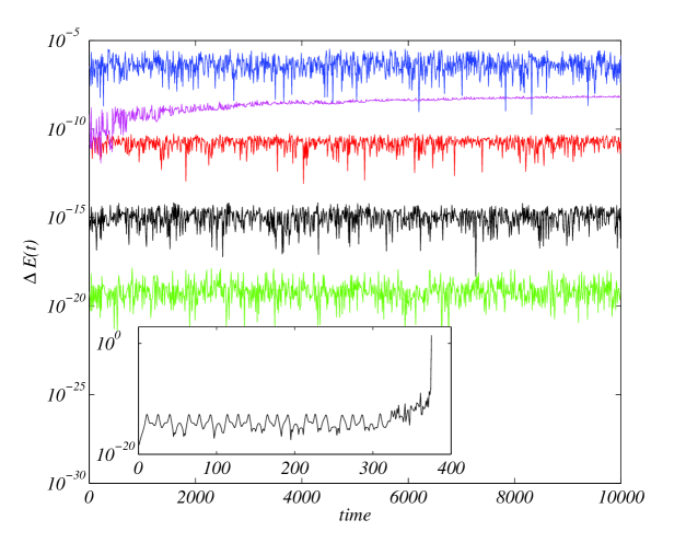
Figure 1. Time evolution of relative energy. Semilog plot of the relative energy loss, $\Delta E(t)=|E(t)-E(0)|/|E(0)|$, as a function of time, for one orbit with initial conditions (22), $N=4$ and a time step $\tau=0.01$. Using, from top to bottom, the integrators $Y_{2}$ (blue), $RK_{4}^{mod}$ (magenta), $Y_{4}$ (red), $Y_{6}$ (black) and $Y_{8}$ (green). Inset : using $RK_{4}$ with time step $\tau=0.001$.

The next study will concern the dependence of the maximum relative energy loss as a function of the time step, by integrating several solutions using $Y_{2m}\left(\tau\right)$, $m\in\{1,2,3,4,5\}$, over a large time span $[0,10^{4}]$; let us observe, once again, that because the relative energy fluctuates around the fixed initial value, the same results hold for arbitrarily longer time spans. Result reported in Fig. 2 shows the computed numerical accuracy of $Y_{2m}\left(\tau\right)$ as a function of the time step $\tau$. Let us observe that the use of $Y_{10}$, respectively of $Y_{8}$, with integration steps $\tau$ smaller than $\sim 2.\,10^{-3}$, respectively $\sim 8.\,10^{-4}$, will produce a maximum relative energy loss below the quadruple machine precision, that is why we limited our simulations to these values. Straight lines reported in Fig. 2 represent linear best fits $\log_{10}\max|\Delta E|=\alpha\log_{10}\tau+\beta$, whose coefficients $\alpha$ and $\beta$ are reported in Table 1 and numerically confirm the accuracy of the integrators $Y_{2m}$.

Let us remark that a similar result holds for larger values of $N$. The main difference being that in this case large time steps are prevented to be used because of a decrease in the performances of all integrator schemes, $Y_{2m}(\tau)$, mainly because of the energy preservation. This fact has been already observed [5] and relies on a stability issue of the integrators, symplectic and non–symplectic ones, that imposes a constrains $\tau N\approx c$, for some positive constant $c$.

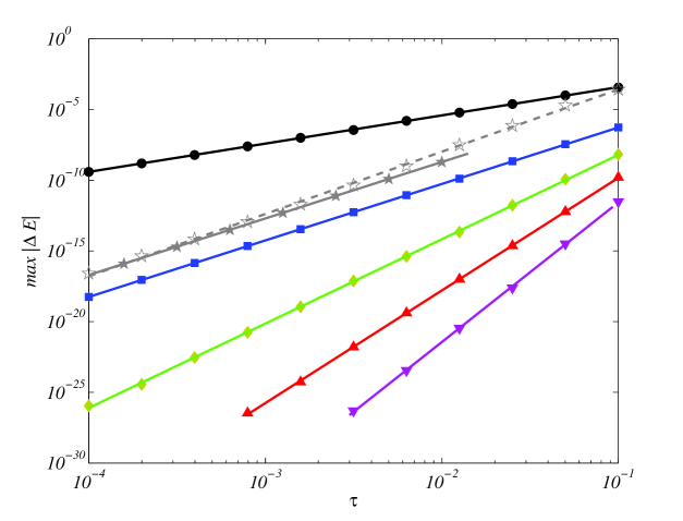
Figure 2. Accuracy of the integrators as a function of $\tau$. We report $\max_{t\in[0,10^{4}]}|\Delta E(t)|$ for orbits with initial conditions given by (22) and $N=4$, numerically integrated over the time span of $[0,10^{4}]$ with $\bigcirc$ $Y_{2}$ (black), $\square$ $Y_{4}$ (blue), $\Diamond$ $Y_{6}$ (green), $\bigtriangleup$ $Y_{8}$ (red), $\bigtriangledown$ $Y_{10}$ (cyan), empty $\star$ $RK_{4}^{mod}$ (grey) and $\star$ $RK_{4}$ (grey) but over a small time span $[0,200]$. Straight lines are linear best fits $\log_{10}\max|\Delta E|=\alpha\log_{10}\tau+\beta$, the coefficients $\alpha$ and $\beta$ are reported in Table 1.

integrator	$\alpha$	$\beta$
$Y_{2}$	$1.997\pm 0.012$	$-1.42\pm 0.03$
$Y_{4}$	$3.996\pm 0.009$	$-2.271\pm 0.023$
$Y_{6}$	$5.97\pm 0.06$	$-2.23\pm 0.15$
$Y_{8}$	$7.97\pm 0.07$	$-1.86\pm 0.16$
$Y_{10}$	$9.88\pm 0.17$	$-1.7\pm 0.3$
$RK_{4}$	$3.997\pm 0.001$	$-0.716\pm 0.006$
$RK_{4}^{mod}$	$4.40\pm 0.11$	$0.82\pm 0.29$

Table 1. Numerical coefficients of the linear best fits $\log_{10}\max|\Delta E|=\alpha\log_{10}\tau+\beta$ reported in Fig. 2.

Our last remark concerns the speed of the numerical methods $Y_{2m}(\tau)$. In Fig. 3 we report the CPU time used to integrate orbits with initial conditions (22) and $N=4$ using $Y_{2m}(\tau)$, as a function of the time step $\tau$. For $Y_{8}$ and $Y_{10}$ we limited the analysis to time steps whose maximum relative energy loss is larger than the machine precision using quadruple precision Fortran (see Fig. 2 and discussion therein). From these data we clearly conclude that the CPU time increases as $1/\tau$ for a fixed integrator scheme $Y_{2m}(\tau)$; on the other hand, for fixed $\tau$, the CPU time increases as a exponential of the integrator order, roughly as $3^{m}$. This is because, as already mentioned, the Yoshida scheme does not get the optimal number of products $\exp(L_{A})$ and $\exp(L_{B})$. On one hand Yoshida already proposed [12] an improved version to tackle this difficulty, whose results are symplectic schemes with fewer compositions (7). Because the computations to obtain the coefficients $(c_{j},d_{j})$ become rapidly cumbersome we limit ourselves to study the cases of sixth order, $Y^{opt}_{6}$, and eighth order, $Y^{opt}_{8}$. Results reported in Fig. 3 show that $Y_{6}(\tau)$ needs almost $1.5$ times more CPU time than $Y^{opt}_{6}(\tau)$, while $Y_{8}(\tau)$ about $2.2$ times more CPU time than $Y^{opt}_{8}(\tau)$.

On the other hand in practical applications one should choose the time step $\tau$ and the integration order $2m$ that produce the best balance between the required precision, say maximum relative energy loss, and the CPU time needed. For instance from Fig. 2 we clearly see that using $Y_{4}$ and $\tau\sim 10^{-3}$, we can ensure a maximum relative energy loss of the order of $10^{-15}$, to get the same precision using $Y_{6}$ one can use a time step ten times larger, $\tau\sim 10^{-2}$ and thus (see Fig. 3) the required CPU time will be smaller with $Y_{6}(10^{-2})$ than with $Y_{4}(10^{-3})$. Requiring the same precision, using instead $Y_{8}$, will need a time step “only”twenty times larger and thus the CPU time will increase: $Y_{8}(2.\,10^{-2})>Y_{6}(10^{-2})$.

The Runge–Kutta 4 requires a CPU time larger than $Y_{4}$ using the same time step, roughly of the same order of $Y_{6}^{opt}$. On the other hand the modified Runge–Kutta scheme is faster than $Y_{4}$ because it has to compute only half of the vector field.

The dependence of the CPU time on the discretization parameter $h$, hence on $N$, is more crucial once we need to use very large $N$ and/or a very large number of orbits. Because in the present work we were not interested in the optimality of the method, we computed “naively”the map $\exp(L_{B})$, namely using a vector–matrix product whose cost is $\mathcal{O}\left(N^{2}\right)$. On the other hand we can easily improve this part by considering the strong similarity with the map $\exp(L_{B})$ and the Fourier transform of the vectors $\left(\vec{p},\vec{q}\right)$ (see Proposition 3.1 and Eq. (18)) and thus use, instead of the vector–matrix product, a Fast Fourier–like method to speed up the computations.

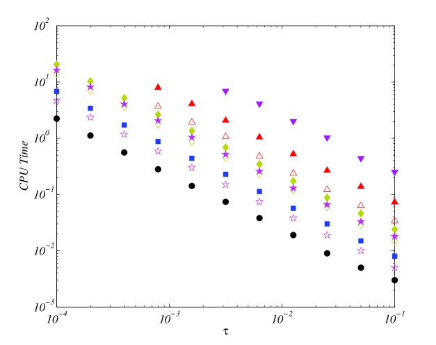
Figure 3. CPU Time needed by $Y_{2m}\left(\tau\right)$ as a function of $\tau$. For a fixed time span of $[0,10^{4}]$ we report the CPU time needed by $Y_{2m}\left(\tau\right)$ to integrate orbits with initial conditions given by (22) and $N=4$. Symbols are : $\bigcirc$ $Y_{2}$ (black), $\square$ $Y_{4}$ (blue), $\Diamond$ $Y_{6}$ (green), empty $\Diamond$ $Y^{opt}_{6}$ (green), $\bigtriangleup$ $Y_{8}$ (red), empty $\bigtriangleup$ $Y^{opt}_{8}$ (red), $\bigtriangledown$ $Y_{10}$ (cyan), empty $\star$ $RK_{4}^{mod}$ (magenta) and $\star$ $RK_{4}$ using (magenta).

5. Conclusions

In this paper we presented a family of high order, explicit, symplectic integrations schemes adapted to the study of the DNLS. Despite DNLS has been studied numerically since long time, this is the first time that such a high precision can be achieved using relatively large time steps. Besides the very good energy preservation properties of the above introduced methods, we also obtained an almost exact preservation of the other first integral, the mass of the system, and of the conjugacy relation. Because the integrators we constructed are explicit ones, they result very fast.

For all these reasons we believe that such accurate numerical schemes could be very useful to test several physical hypotheses concerning the asymptotic regimes of the DNLS, for instance the existence and stability of breathers and the regimes with negative temperature.

References

- [1] P.J. Channel and C. Scovel, Symplectic integration of Hamiltonian systems, Nonlinearity, 3, (1990), pp. 231.
- [2] Davis P.R., Circulant Matrices, (1979), John Wiley, New York.
- [3] S. Flach, D. O. Krimer, and Ch. Skokos, Universal Spreading of Wave Packets in Disordered Nonlinear Systems, Phys. Rev. Lett., 102, (2009), pp. 024101.
- [4] E. Hairer, C. Lubic and G. Wanner, Geometric Numerical Integration. Structure–preserving Algorithms for ordinary differential equations, 2nd Ed. Springer (2006), Springer–Verlag, Berlin Heidelberg.
- [5] D.A. Karpeev and C.M. Schober, Symplectic integrators for discrete nonlinear Schrodinger systems, Mathematics and Computers in Simulations, 56, (2001), pp. 145.
- [6] P.G. Kevrekidis, The Discrete Nonlinear Schrödinger Equation, STMP 232, (2009), Springer-Verlag Berlin Heidelberg.
- [7] R.I. McLachlan and P. Atela, The accuracy of symplectic integrators, Nonlinearity, 5, (1992), pp. 541.
- [8] J. Laskar and Ph. Robutel, High order symplectic integrators for perturbed hamiltonian systems, Cel. Mec. , , (2001), pp. 39–62.
- [9] M.A. Porter, Experimental Results Related to DNLS Equations, in P.G. Kevrekidis: The Discrete Nonlinear Schrödinger Equation. Mathematical analysis, Numerical Computations and Physical Perspectives, STMP, 232, Springer-Verlag Berlin Heidelberg (2009), pp.175
- [10] C.M. Schober, Symplectic integrators for the Ablowitz–Ladik discrete nonlinear Schrod̈inger equation, Phys. Lett. A, 259, (1999), pp. 140.
- [11] Ch. Skokos, D.O. Krimer, S. Komineas and S. Flach, Delocalization of wave packets in disordered nonlinear chains, Phys. Rev. E, 79, (2009), pp. 056211.
- [12] H. Yoshida, Construction of higher order symplectic integrators, Physics Letters A, 150, 5,6,7, (1990), pp. 262.