The WSRT Virgo H i filament survey I

Abstract

Context. Observations of neutral hydrogen can provide a wealth of information about the kinematics of galaxies. To learn more about the large scale structures and accretion processes, the extended environment of galaxies have to be observed. Numerical simulations predict a cosmic web of extended structures and gaseous filaments.

Aims. To observe the direct vicinity of galaxies, column densities have to be achieved that probe the regime of Lyman limit systems. Typically H i observations are limited to a brightness sensitivity of $N_{HI}\sim 10^{19}$ cm^-2 but this has to be improved by $\sim 2$ orders of magnitude.

Methods. With the Westerbork Synthesis Radio Telescope (WSRT) we map the galaxy filament connecting the Virgo Cluster with the Local Group. About 1500 square degrees on the sky is surveyed, with Nyquist sampled pointings. By using the WSRT antennas as single dish telescopes instead of the more conventional interferometer we are very sensitive to extended emission.

Results. The survey consists of a total of 22,000 pointings and each pointing has been observed for 2 minutes with 14 antennas. We reach a flux sensitivity of 16 mJy beam^-1 over 16 km s^-1, corresponding to a brightness sensitivity of $N_{HI}\sim 3.5\times 10^{16}$ cm^-2 for sources that fill the beam. At a typical distance of 10 Mpc probed by this survey, the beam extent corresponds to about 145 kpc in linear scale. Although the processed data cubes are affected by confusion due to the very large beam size, we can identify most of the galaxies that have been observed in HIPASS. Furthermore we made 20 new candidate detections of neutral hydrogen. Several of the candidate detections can be linked to an optical counterpart. The majority of the features however do not show any signs of stellar emission. Their origin is investigated further with accompanying H i surveys which will be published in follow up papers.

1 Introduction

Unbiased, wide-field sky surveys are very important in improving understanding of our extended extragalactic environment. They provide information about the clustering of objects and the resulting large scale structures. Furthermore, they are essential in providing a complete sample of galaxies, their mass function and physical properties. Several outstanding examples are the SDSS (Sloan Digital Sky Survey) (York et al., 2000) at optical wavelengths, and HIPASS (H i Parkes All Sky Survey) (Barnes et al., 2001) and ALFALFA (The Arecibo Legacy Fast ALFA Survey) (Giovanelli et al., 2005) in the 21cm line of neutral hydrogen. All these surveys have been important milestones, that significantly improved our understanding of the distribution of galaxies in the universe. But despite the impressive results, these surveys can only reveal the densest structures in the Universe like galaxies, groups and clusters.

In the low redshift Universe, the number of detected baryons is significantly below expectations, indicating that not all the baryons are in galaxies. According to cosmological measurements the baryon fraction is about 4$\%$ at $z\sim 2$ (Bennett et al. (2003); Spergel et al. (2003)). This is consistent with actual numbers of baryons detected at $z>2$ (Weinberg et al. (1997); Rauch (1998)). In the current epoch however, at $z\sim 0$ about half of this matter has not been directly observed (Fukugita et al. (1998); Cen & Ostriker (1999); Tripp et al. (2000); Savage et al. (2002); Penton et al. (2004)).

Recent hydrodynamical simulations give a possible solution for the “Missing Baryon” problem (Cen & Ostriker (1999); Davé et al. (2001); Fang et al. (2002)). Not all the baryons are in galaxies, that are just the densest concentrations in the Universe. Underlying them is a far more tenuous Cosmic Web, connecting the massive galaxies with gaseous filaments. The simulations predict that at $z$ = 0 cosmic baryons are almost equally distributed amongst three phases (1) the diffuse IGM, (2) the warm hot intergalactic medium (WHIM), and (3) the condensed phase. The diffuse phase is associated with warm, low-density photo-ionized gas. The WHIM consists of gas with a moderate density, that has been heated by shocks during structure formation. The WHIM has a very broad temperature range from $10^{5}$ to $10^{7}$ K. The condensed phase is associated with cool galactic concentrations and their halos. These three components are each coupled to a decreasing range of baryonic over-density: log$(\rho_{H}/\bar{\rho_{H}})$ $<$ 1, 1–3.5, and $>$ 3.5 and are probed by QSO absorption lines with specific ranges of neutral column density: log$(N_{HI})$ $<$ 14, 14–18 and $>$ 18 (Braun & Thilker, 2005).

1.1 Cosmic Web

The Warm Hot Intergalactic Medium is thought to be formed during structure formation. Low density gas is heated by shocks during its infall onto the filaments that define the large scale structure of the Universe. Most of these baryons are still concentrated in unvirialized filamentary structures of highly ionized gas.

The WHIM has been observationally detected in QSO absorption line spectra using lines of NeVIII (Savage et al. 2005), OVI (e.g. Tripp et al. 2008), broad Ly$\alpha$ (Lehner et al. 2007) and X-ray absorption (Nicastro et al., 2005). Of course, absorption studies alone do not give us complete information on the spatial distribution of the WHIM. Emission from the Cosmic Web would give entirely new information about the distribution and kinematics of the intergalactic gas.

Direct detection of the WHIM is very difficult in the EUV and X-ray bands (Cen & Ostriker, 1999). The gas is ionized to such a degree, that it becomes “invisible” in infrared, optical or UV light, but should be visible in the FUV and X-ray bands (Nicastro et al., 2005). Given the very low density, extremely high sensitivity and a large field of view is needed to image the filaments. Capable detectors are not yet available for the X-ray or FUV (Yoshikawa et al. (2003); Nicastro et al. (2005)).

Due to the moderately high temperature in the intergalactic medium (above $10^{4}$ Kelvin), most of the gas in the Cosmic Web is highly ionised. To detect the trace neutral fraction in the photoionized Ly$\alpha$ forest using the 21-cm line of neutral hydrogen, a column density sensitivity of $N_{HI}\sim 10^{17-18}$ cm^-2 is required. At the current epoch we can confidently predict that in going down from H i column densities of $10^{19}$ cm^-2 (which define the current ”edges” of well studied nearby galaxies in H i emission) to $10^{17}$ cm ^-2 the surface area will significantly increase, as demonstrated in Corbelli & Bandiera (2002), Braun & Thilker (2004) and Popping et al. (2009).

The critical observational challenge is crossing the “H i desert”, the range of log($N_{HI}$) from about 19.5 down to 18 over which photo-ionization by the intergalactic radiation field produces an exponential decline in the neutral fraction from essentially unity down to a few percent (eg. Dove & Shull (1994)). Nature is kinder again to the H i observer below log(N_HI) = 18, where the neutral fraction decreases only very slowly with log($N_{HI}$). The neutral fraction of hydrogen is thought to decrease with decreasing column density from about 100$\%$ for $\log(N_{HI})$ $\>=$ 19.5 to about 1$\%$ at $\log(N_{HI})=17$ (Dove & Shull, 1994). The baryonic mass traced by this gas is expected to be comparable to that within the galaxies, as noted above.

To detect the peaks of the Cosmic Web in H i, a blind survey is required that covers a significant part of the sky, of the order of at least 1000 square degrees. Furthermore a brightness sensitivity is required that is about an order of magnitude more sensitive than HIPASS.

The Westerbork Synthesis Radio Telescope (WSRT) has been used to undertake a deep fully sampled survey mapping $\sim 1300$ square degrees of sky. The survey covers a slab perpendicular to the plane of the local supercluster, centred on the galaxy filament connecting the Local Group with the Virgo Cluster. Due to our observing strategy with declinations between $-$1 and 10 degrees and a limited velocity range, the survey does not encompass the complete Virgo cluster. In an unbiased search for diffuse and extended H i gas, both the auto-correlation and cross-correlation data are reduced and analysed. In this paper we will only discuss the total-power product, as this product is most sensitive to faint and extended emission. The resulting detections will be further analysed and compared with the cross-correlation data products and other data in subsequent papers.

We have achieved an RMS sensitivity of about 16 mJy Beam^-1 at a velocity resolution of 16 km s^-1 over $\sim 1300$ deg² and between $400<V_{Hel}<1600$ km s^-1. The corresponding RMS column density for emission filling the $2983\times 2956$ arcsec effective beam area is $\sim 3.5\times 10^{16}$ cm^-2 over 16 km s^-1. Although the flux sensitivity is similar to HIPASS, that has typically achieved 13.5 mJy Beam^-1 at a velocity resolution of 18 km s^-1, the column density sensitivity is far superior. With the 14 arcmin intrinsic beam size of the Parkes telescope, the RMS column density sensitivity in HIPASS is $\sim 4\times 10^{17}$ cm^-2 over 18 km s^-1, which is more than an order of magnitude less sensitive.

In the Westerbork Virgo Filament Survey we detect 129 sources that are listed in the HIPASS catalogue. We have made 20 new H i detections, of which many do not have a clear optical counterpart. The outline of this paper is as follows: in Sect. 2 we describe the survey observations and strategy, directly followed by the reduction procedures of the auto-correlation data. In Sect. 4 we present the results of H i detections of known galaxies and the new detections. We end with a short discussion and conclusion in Sect. 5. The results of the cross-correlation data of the Westerbork Virgo Filament Survey and the detailed analysis and data comparison will be presented in two subsequent papers.

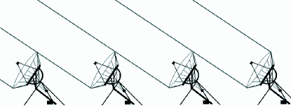
Figure 1: Observing mode of the WSRT dishes; a filled aperture of 300 m is simulated by placing 12 of the 14 telescopes at regular intervals and observing only at extreme hour angles.

2 Observations

To obtain the highest possible brightness sensitivity in cross-correlations, the WSRT was configured to simulate a large filled aperture in projection. Twelve of the 14 WSRT 25 m telescopes were positioned at regular intervals of 144 m. When observing at very low declinations and extreme hour angles, a filled aperture is formed (as can be seen in Fig. 1), which is 300 $\times$ 25 m in projection. In this peculiar observing mode the excellent spectral baseline and PSF properties of the interferometer are still obtained while achieving excellent brightness sensitivity. A deep fully-sampled survey of the galaxy filament joining the Local Group to the Virgo Cluster has been undertaken, extending from 8 to 17 hours in RA and from $-$1 to +10 degrees in declination and covering 40 MHz of bandwidth with 8 km s^-1 resolution.

Simultaneously with the cross-correlation data, auto-correlation data was acquired. These auto-correlation data pertain to the same set of positions on the sky. Data were acquired in a semi-drift-scan mode, whereby the 25 m telescopes of the WSRT array tracked a sequence of positions for a 60 s integration that were separated by one minute of right ascension (about 15 arcmin) yielding Nyquist-sampling in the scan direction of the telescope beam. Data was acquired in two 20 MHz IF bands centered at 1416 and 1398 MHz. The beamwidth of each telescope is $38\times 37$ arcmin FWHM at an observing frequency of 1416 MHz.(Popping & Braun, 2008). Each drift-scan sequence, lasting about 9 hours, was separated by 15 arcmin in declination to give Nyquist sampling. Typically, an observing sequence consisted of a standard observation of a primary calibration source (3C48 or 3C286) a drift-scan observation and an additional primary calibration source. Each session provided a strip of data of $135\times 0.25$ true degrees. In total 45 of these strips provided the full survey coverage of 11 degrees in declination. Each of the total of 24,300 pointings was observed two times, once when the sources were rising and once when they were setting. The total of 90 sessions were distributed over a period of more than two years, between December 2004 and March 2006.

Although the observations cover a large bandwidth in each of two bands, we only use the radial velocity range from 400 to 1600 km s^-1 in the first band. For lower radial velocities, the emission is too confused with Galactic emission and combined with the very large beam size, useful analysis was deemed impractical. The second IF band with a lower central frequency samples larger distances, where the central frequency corresponds to a Hubble-flow distance of about 65 Mpc. The physical beam size at this distance is about 850 kpc. Detecting emission which fills such a large beam would be very unlikely, while the problem of confused detections is more serious.

To minimize solar interference, an effort was made to measure the data only after local sunset and before local sunrise. Unfortunately this was not successful for the whole survey and a few runs show the effects of solar interference.

3 Data reduction

Auto-correlation and Cross-correlation data were acquired simultaneously, and were separated before importing them into Classic AIPS (Fomalont, 1981). We will now only describe the steps that have been undertaken to reduce the auto-correlation or total-power data. The reduction method for the cross-correlation data is significantly different and will be described in another publication.

Every baseline of the drift-scan data of each survey run was inspected and flagged in Classic AIPS, using the SPFLG utility. Suspicious features appearing in the frequency or time display of each auto-correlation baseline were critically inspected. This was accomplished by comparing the 28 independent spectral estimates resulting from 14 telescopes, each with two polarizations. Features which could not be reproduced in the simultaneous spectra were flagged.

Absolute flux calibration of the data was provided by the observed mean cross-correlation coefficient measured for the standard calibration sources (3C48 or 3C286) of known flux density. The measured ratio of flux density to correlation coefficient averaged over all 14 telescopes and 2 polarizations was $340\pm 10$ Jy/Beam.

Two different methods were employed to generate data-cubes of the auto-correlation data. The main difficulty with total power data, is obtaining a good band-pass calibration. The first method employed taking a robust average of a 30 min sliding window, to estimate the band-pass as a function of time and an 850 km s^-1 sliding window to estimate the continuum level as a function of frequency. Only the inner three quartiles of the values were included in these averages, making them moderately robust to outliers, including H i emission features, in the data. The big advantage of this method is that it could be applied blindly in a relative fast way, and it produces uniform noise characteristics in the resulting cube. In this way, it is very suitable for detecting faint and diffuse sources. However the disadvantage is that bright sources with a moderately high level of H i emission that are extended in either the spatial or velocity direction produce a local negative artifact. Under these circumstances, better results are obtained with a more complicated and time consuming method, described below.

The result of the first bandpass-removal method has been used to create a mask. For each declination the clearly recognisable bright sources that correspond to galaxies were included by hand. In the mask, the location of the galaxies was set to zero and the rest of the declination scan was set to unity. The mask was applied to the raw data, so only the noise, diffuse sources and the bandpass characteristics remain. A second order polynomial was then fit in the frequency direction and the masked data is divided by this polynomial result. In the next step a zeroth order polynomial is fit in the time domain and the masked data is divided by this product. Finally a third order polynomial is applied again in the frequency domain, to remove small oscillations or artifacts. Within each declination strip a correction has been applied to correct for the Doppler shift at the time of the observation before combining the declinations and creating a three dimensional cube. The improvement in using the second method for the bandpass correction is shown in Fig. 2. In the left panel bright sources can be easily identified, however there are large negative spectral artifacts at the source location. By masking the regions of bright emission, a much better bandpass estimate could be achieved that does not suffer from artifacts as can be seen in the right panel of Fig. 2.

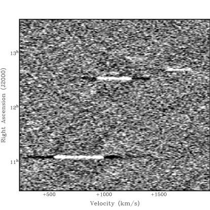
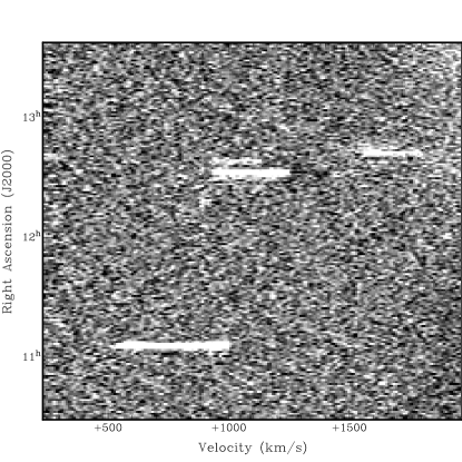
Figure 2: Illustration of the bandpass correction method. In the left panel a robust average over a sliding window in both frequency and position is used to identify the brightest sources of emission. In the right panel the bright sources have been individually masked before carrying out a polynomial fit. Both panels show the same region (declination is zero) with the same intensity scale.

3.1 Doppler Correction

The drift-scan data were resampled in frequency to convert from the fixed geocentric frequencies of each observing date to a heliocentric radial velocity at each observed position. The offsets in velocity have been determined using the reference coordinate utilities within aips++. This correction depends on the earth’s velocity vector relative to the pointing direction at the time of an observation and varies between about $-$30 and +30 km s^-1 during the course of a year. Since the observations have been undertaken over a time span of several years, this effect has to be taken into account.

3.2 Calibration

Due to the extreme hour angles and low declinations of the observations, there is a larger intervening airmass (between 1.35 and 1.7) and increased ground pick-up effecting the observed emission than in a typical observation. While the attenuation of the astronomical signal is minimal (less than 2%) in view of the low zenith opacity at the observing frequency, the system temperature increases significantly. This increase is measured directly by comparison with a periodically injected noise signal of known temperature and can be understood in terms of a combination of atmospheric emission and the extended far-sidelobe pattern of the telescope response convolved with the telescope environment. As a result, the system temperature $(T_{sys})$ of the survey scans was higher than for the calibrator sources. This effect has to be taken into account when doing the gain-calibration to get correct flux values. In Fig. 3 this correction factor is plotted as function of declination, based on the ratio of system temperatures seen in the survey scans relative to the associated calibration scans. The correction that has to be applied is strongly correlated with declination (since this is directly coupled to elevation); at the lowest declination of $-$1 degrees, the gains have to be multiplied by a factor $\sim 1.6$ to get correct flux values. The minimum correction is near 7.5 degrees. The slight increase in the ratio at higher declinations may be due to increasing ground pick-up in the spill-over lobe of the telescope illumination pattern. The scans that observe the setting of the sources have a slightly higher correction factor. Antenna 1 (locally known as RT0) suffered from severe blockage by the trees to the west of the array at these extreme hour angles and therefore it has not been used. The gain corrections can be fit using a second order polynomial. These corrections have been applied independently to both the rise and set data.

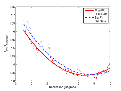
Figure 3: Due to the extreme hour angles at which the observations were taken, there is an increased system temperature with respect to the calibrators. This correction is dependent on the declination. The dash-dotted line represents the calibration factors for the rise data with the best second order polynomial fit shown as a solid line. The dotted line corresponds to the set data, with the fit shown as a short-dashed line.

3.3 Data Cubes

The 45 drift-scans of both the setting and rising data were combined into two separate data cubes and exported to the MIRIAD software package (Sault et al., 1995). A combined cube was obtained by taking the RMS-weighted average of the two independent cubes containing all the data. This cube combines two fully independent surveys of the same region. A spatial convolution was applied to all three cubes with a 2000 arcsec FWHM Gaussian with PA=0 to introduce the desired degree of spatial correlation in the result. A hanning smoothing was applied with a width of three pixels to smooth the cubes in the velocity domain, resulting in a velocity resolution of 16 km s^-1.

3.4 Sensitivity

After creating cubes of the combined and individual rise and set data, sub-cubes were created, excluding Galactic emission and excluding the edge of the bandpass. The noise in the rise-data is 22 mJy beam^-1 over 16 km s^-1, while the noise in the set-data is slightly worse, 23 mJy beam^-1 over 16 km s^-1. The noise in the combined data cubes is 16 mJy beam^-1 over 16 km s^-1, which is in agreement with what would be expected, as the noise improves with exactly a factor $\sqrt{2}$. In Fig. 4 a histogram is plotted of the flux values in the combined data cube. On the positive side the flux values are dominated by real emission, however a Gaussian can be fitted to the noise at negative fluxes. The noise appears to be approximately Gaussian with a dispersion of 16 mJy beam^-1. There is however some dependance of the RMS values on declination as shown in Fig. 5. When observing a specific declination strip, there is not much difference in the noise at different right ascensions or in the frequency domain, as all data points have been obtained under similar circumstances. Since the declinations strips have been observed on different days, some real fluctuation in the noise is more likely. We can see a scatter in the noise for different declinations of 5 to 10 percent. Furthermore, there is a general trend that the lowest declinations have the highest noise values, which is expected due to a higher system temperature at these lowest declinations (as demonstrated in Fig. 3).

The flux sensitivity can be converted to a brightness temperature using the equation:

$$T_{b}=\frac{\lambda^{2}S}{2k\Omega}$$ (1)

where $\lambda$ is the observed wavelength, $S$ is the flux density, $k$ the Boltzmann constant and $\Omega$ is the beam solid angle of the telescope. When using the 21 cm line of H i, this equation can be written as:

$$T_{b}=\frac{606}{b_{min}b_{maj}}S$$ (2)

where $b_{min}$ and $b_{maj}$ are the beam minor and major axis respectively in arcsec and $S$ is the flux in units of mJy/Beam. The total flux can be converted into an H i column density assuming negligible self-opacity using:

$$N_{HI}=1.823\cdot 10^{18}\int T_{b}dv$$ (3)

with $[N_{HI}]$ = cm^-2, $[T_{b}]$ = K and $[dv]$ = km s^-1, resulting in a column density sensitivity of $3.5\cdot 10^{16}$ cm^-2 over 16 km s^-1.

We emphasise that the stated column density limit assumes emission completely filling the beam. This can only be achieved, if the emitting structure is larger than the beam. Observations described in this paper can only resolve very extended structures and have reduced sensitivity to compact features like dwarf galaxies or the inner parts of large galaxies. Emission from compact structures will be diluted to the full size of the beam and a better angular resolution is required to distinguish compact from extended emission.

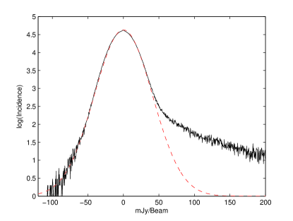
Figure 4: Histogram of the occurrence of brightnesses in the combined data cube on a logarithmic scale. The high brightnesses are dominated by significant emission, but the noise at low brightnesses can be fitted with a Gaussian function with a dispersion that closely agrees with the RMS value in emission-free regions.

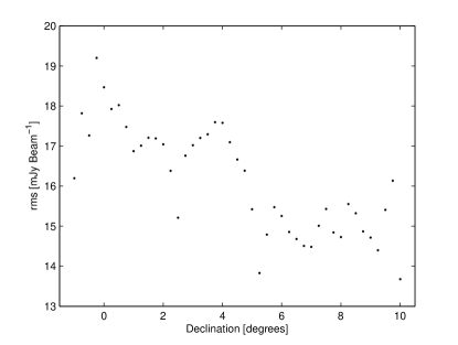
Figure 5: Differences in RMS noise as function of declination. There is some scatter due to different conditions, since each declination is observed on a different date. In general low declinations have a slightly elevated noise value, due to an increased system temperature at the lowest declinations.

4 Results

Due to the very large beam of the observations it is impossible to determine the detailed kinematics of detected objects. Small and dense objects cannot be distinguished from diffuse and extended structures as the emission of compact sources will be spatially diluted to the large beam size. Nevertheless, the total power product of the survey is still a very important one, as it provides the best H i brightness sensitivity over such a large region for intrinsically diffuse structures. There are other surveys with a comparable flux sensitivity, but with a much smaller beam. These observations would need to be dramatically smoothed in the spatial domain to get a similar column density sensitivity as our survey. The diffuse emission we seek is hidden in the noise at the native resolution and can easily be affected by bandpass corrections or other steps in the reduction process. In general, an H i observation is most sensitive to structures with a size that fill the primary beam of a single dish observations or the synthesized beam of interferometric data.

We detect many galaxies in the filament connecting the Virgo Cluster with the Local Group. Detailed analysis of known galaxies is not very interesting at this stage, as there are other H i surveys like HIPASS and ALFALFA that have observed the same region with much higher resolution. These surveys, or deep observations of individual galaxies are much more suitable to analyse the physical parameters of these objects. In the Total Power product of the WVFS we are interested in emission that can not or has not been detected by previous observations, because it is below their brightness sensitivity limit.

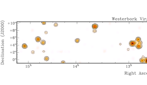
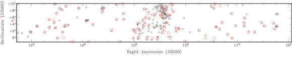
Figure 6: Illustration of the central 110 degrees of the WVFS region and detections in the velocity interval $400<V_{Hel}<1600$ km s^-1. The top panel shows the integrated brightness levels, with contour levels drawn at 5, 10, 20, 40, 80 and 160 Jy Beam^-1 km s^-1. Note that contour levels are chosen very conservatively and do not include faint emission near the noise floor. The second panel shows the position of all known H i-detected galaxies (small black circles) within the redshift range of the WVFS data with the WVFS detections overlaid (large red circles).

An overview of the central 110 degrees in Right Ascension of the survey sky coverage is given in Fig. 6 together with contours of the brightest emission. The image shows the zeroth moment map integrating the velocity interval $400<V_{Hel}<1600$ km s^-1. Contour levels are drawn at 5, 10, 20, 40, 80 and 160 Jy Beam^-1 km s^-1. The second panel shows the location of galaxies for which H i has been detected previously within the same redshift interval as the WVFS total-power data (small black circles), all WVFS detections are indicated by large red circles. The known galaxies where selected from the HyperLeda (Paturel et al., 1989) database, by looking for galaxies with a known H i component within the spatial and spectral range of WVFS. While we do detect most known galaxies, the survey suffers from confusion, especially in the densely populated central part of the survey region. When multiple galaxies with overlapping velocity structures are within one beam, these result in only one detection. A couple of galaxies for which H i has been detected before are not found in our data, when carefully looking into the data cubes for some cases a tentative signal can be observed, however this does not reach a three $\sigma$ level as the H i flux is too much diluted by the large beam.

An attempt was made to detect sources using the source finding algorithm Duchamp (Whiting, 2008) and by applying masking algorithms within the MIRIAD (Sault et al., 1995) and GIPSY (van der Hulst et al., 1992) software packages. None of these automatic methods appeared to be practical due to the very large intrinsic beam size of the data. All sources are unresolved and there is a lot of confusion between sources at a similar radial velocity where the angular separation is smaller than the beam-width.

A list of candidate sources was determined from visual inspection of subsequent channel maps, using the KVIEW task in the KARMA package (Gooch, 1996). The combined cube containing both the rise and set data, as well as the individual rise and set cubes were each inspected. Features were accepted if local peaks exceeded the 3$\sigma$ limit in at least two subsequent channels in the combined data cube and if they exceeded the 2$\sigma$ limit in the individual rise and set data products. This cutoff level is very low, however the rise and set data represent two completely independent observations undertaken at different times, giving extra confidence in the resulting candidates. Furthermore we are looking for diffuse extended structures, which are expected to occur at those low flux levels. Using a high clipping level will significantly reduce the chances for including such diffuse emission features in an initial candidate list.

In total we found 188 candidate sources of which the properties are estimated in detail. The integrated line strengths have been determined for each candidate by extracting the single spectrum with the highest flux density from both the rise and set cube. As there were artifacts in the bandpass, a second order polynomial has been fitted to the bandpass and was subtracted from the spectra. The average of the two integrated line strengths was determined to get the best solution. We assume here that all detections are unresolved when using an effective FWHM beamsize of $2982\times 2956$ arcsec.

Subsequently all candidate detections have been compared with catalogued detections in the H i Parkes All Sky Survey. The HIPASS database completely covers our survey region and currently has the best column density sensitivity.

The list of candidate detections is split into two parts. Detections with an HIPASS counterpart at a similar position and velocity can be confirmed and are reliable detections. In total, 129 of our candidates could be identified in the HIPASS catalogue. When taking into account the expected overlap of HIPASS objects in our larger spatial beam, we confirm 146 of the 149 HIPASS detections in this region. The remaining 58 WVFS candidates have not been catalogued in HIPASS.

The corresponding error in flux density was determined over a velocity interval of $1.5\times W_{20}$, where $W_{20}$ is the velocity width of the emission profile at 20% of the peak intensity and is given by:

$$\sigma=\sqrt{\frac{1.5\cdot W_{20}}{v_{res}}}\cdot\delta v\cdot rms$$ (4)

Rosenberg & Schneider (2002) have shown that in surveys of this type, an asymptotic completeness of about 90% is reached at a signal-to-noise ratio of 8, when considering the integrated flux. Comparison with the noise histogram shown in Fig. 4 demonstrates that no negative peaks occur which exceed this level, suggesting that the incidence of false positives should also be minimal. When we adopt this limit, only 20 detections, with an integrated flux density exceeding 8 times the associated error remain from the 58 candidates.

We will mention the candidate detections here and give their general properties, however we leave further analysis to a subsequent paper, when we incorporate the cross-correlation data and an improved version of the HIPASS product for comparison. We emphasise here that although the detections seem obvious in the total-power data at the 8$\sigma$ level, they are considered as candidate detections. They have to be analysed and compared using other data-sets, to be able to confirm the detections and make strong statements.

4.1 Source Properties of Known Detections

The properties of all previously known H i detections are summarised in table LABEL:conf_det. The first column gives the names of the source as given in the Westerbork Virgo Filament Survey. The name consists of the characters “WVFS” followed by the right ascension of the object in [hh:mm] and the declination in [d:mm]. The second column gives the more common name of objects for which we have identified the H i counterpart. In the third and forth column the RA and Dec positions are given, followed by the estimated heliocentric recession velocity in the fifth column. In the last two columns we give the integrated flux in [Jy-km s^-1] and the $W_{20}$ line width in [km s^-1]. Spectra of all the confirmed H i detections are shown in the appendix of this paper.

Several of the detections are at the edge of the frequency coverage of the cube and are indicated with an asterisk in the table in the column with the $W_{20}$ values. The observed spectrum for these sources is not complete, which results in only a lower limit to the integrated flux. We will not consider these sources in our further analysis.

Table 1: Physical properties of confirmed detections in the Westerbork Virgo Filament Survey total-power data.

Name	Optical ID.	RA [hh:mm:ss]	Dec [dd:mm]	$V_{Hel}$ [km s-1]	$S$ [Jy km s-1]	$W_{20}$ [km s-1]
WVFS 0906+0615	UGC 4781	09:06:27	6:15	1419	15.0	234
WVFS 0908+0515	SDSS J090836.54+051726.8	09:08:27	5:15	597	1.2	50
WVFS 0908+0600	UGC 4797	09:08:27	6:00	1285	4.2	120
WVFS 0910+0700	NGC 2775	09:10:27	7:00	1491	9.7	160
	NGC 2777
WVFS 0943-0045	UGC 5205	09:43:33	-0:45	1501	8.1	115
WVFS 0943+0945	IC0559	09:43:33	9:45	522	6.2	150
WVFS 0944-0045	SDSS J094446.23-004118.2	09:44:32	-0:45	1194	4.2	150
WVFS 0951+0745	UGC 5288	09:51:34	7:45	539	25.9	120
WVFS 0953+0130	NGC3044	09:53:34	1:30	1300	35.6	330
WVFS 0954+0915	NGC 3049	09:54:35	9:15	1469	13.5	230
WVFS 1013+0330	NGC 3169	10:13:38	3:30	1200	110.7	510
WVFS 1013+0700	UGC 5522	10:13:38	7:00	1194	40.4	235
WVFS 1016+0245	UGC 5539	10:16:38	2:45	1251	9.1	210
WVFS 1017+0415	UGC 5551	10:17:38	4:15	1302	5.5	120
WVFS 1027+0330	UGC 5677	10:27:40	3:30	1169	6.1	130
WVFS 1031+0430	UGC 5708	10:31:41	4:30	1144	30.0	210
WVFS 1039+0145	UGC 5797	10:39:42	1:45	671	4.4	110
WVFS 1046+0145	NGC 3365	10:46:43	1:45	945	42.5	265
WVFS 1050+0545	NGC 3423	10:50:44	5:45	988	34.7	185
WVFS 1051+0330	PGC 2807138	10:51:44	3:30	1053	13.1	105
WVFS 1051+0415	UGC 5974	10:51:44	4:15	1030	11.6	180
WVFS 1101+0330	NGC 3495	11:01:46	3:30	1028	27.5	330
WVFS 1105+0000	NGC 3521	11:05:46	0:00	704	275.8	480
WVFS 1105+0715	NGC 3526	11:05:46	7:15	1418	6.0	205
WVFS 1110+0100	CGCG 011-018	11:10:47	1:00	969	4.3	75
WVFS 1117+0430	NGC 3604	11:17:48	4:30	1527	3.2	120
WVFS 1119+0930	SDSS J111928.10+093544.2	11:19:49	9:30	961	1.5	40
WVFS 1120+0245	UGC 6345	11:20:48	2:45	1568	9.6	100
WVFS 1124+0315	NGC 3664	11:24:29	3:15	1380	19.0	160
WVFS 1125+1000	IC 0692	11:25:49	10:00	1127	2.8	80
WVFS 1126-0045	UGC 6457	11:26:49	-0:45	937	4.6	90
WVFS 1126+0845	IC 2828	11:26:50	8:45	1011	3.9	90
WVFS 1129+0915	NGC3705	11:29:50	9:15	1019	51.5	360
WVFS 1136+0045	UGC 6578	11:36:51	0:45	1022	5.4	115
WVFS 1143+0215	PGC 036594	11:43:52	2:15	976	5.6	55
WVFS 1200-0100	NGC 4030	12:00:55	-01:00	1418	39.5	360
WVFS 1207+0245	NGC 4116	12:07:56	2:45	1285	89.5	230
	NGC 4123
WVFS 1210+0200	UGC 7178	12:10:56	2:00	1302	10.9	100
WVFS 1210+0300	UGC 7185	12:10:57	3:00	1269	13.6	150
WVFS 1213+0745	UGC 7239	12:13:57	7:45	1194	7.6	140
WVFS 1215+0945	NGC 4207	12:15:58	9:45	599	5.1	180
WVFS 1216+1000	UGC 7307	12:16:57	10:00	1152	2.7	65
WVFS 1217+0030	UGC 7332	12:17:58	0:30	911	19.1	85
WVFS 1217+0645	NGC 4241	12:17:58	6:45	704	8.5	140
WVFS 1219+0645	VCC 0381	12:19:58	6:45	456	1.4	40∗
WVFS 1219+0130	UGC 7394	12:19:58	1:30	1552	3.4	125
WVFS 1221+0430	NGC 4301	12:21:59	4:30	1252	20.2	135
WVFS 12222+0915	NGC 4316	12:22:58	9:15	1244	7.1	365
WVFS 1222+0430	M 61	12:22:00	4:30	1535	95.8	185
WVFS 1222+0815	NGC 4318	12:22:59	8:15	1402	2.8	90
WVFS 1223+0215	UGC 7512	12:24:59	2:15	1477	4.1	95
WVFS 1224+0315	pgc 040411	12:24:59	3:15	900	10.1	85
WVFS 1225+0545	VCC 0848	12:25:59	5:45	1110	13.9	175
	NGC 4376
	NGC 4423
WVFS 1225+0715	IC 3322A	12:25:59	7:15	1078	8.7	115
WVFS 1225+0900	NGC 4411	12:25:59	9:00	1236	20.9	110
	NGC 4411 b
WVFS 1226+0130	pgc135803	12:26:59	1:30	1265	43.3	110
WVFS 1226+0715	UGC 7557	12:26:59	7:15	920	31.9	175
WVFS 1227+0615	NGC 4430	12:27:59	6:15	1402	2.7	120
WVFS 1227+0845	UGC 7590	12:27:59	8:45	1053	4.6	95
WVFS 1228+0645	IC 3414	12:28:59	6:45	497	4.8	130∗
WVFS 1229+0245	UGC 7612	12:29:30	2:45	1595	16.6	170
	UGC 7642
WVFS 1230+0930	HIPASS J1230+09	12:30:00	9:30	473	5.6	120∗
WVFS 1233+0000	NGC 4517	12:33:01	0:00	1078	124.1	325
WVFS 1233+0030	NGC 4517A	12:33:01	0:30	1510	31.7	175
WVFS 1233+0845	NGC 4519	12:33:01	8:45	1186	51.8	220
WVFS 1236+0630	IC 3576	12:36:01	6:30	1045	15.2	70
WVFS 1237+0315	UGC 07780	12:37:01	3:15	1410	3.0	130
WVFS 1237+0700	IC 3591	12:37:01	7:00	1593	10.4	120∗
WVFS 1239-0030	NGC 4592	12:39:02	-00:30	1061	127.5	220
WVFS 1243+0345	NGC 4630	12:43:01	3:45	696	6.8	160
WVFS 1243+0545	VCC 1918	12:43:02	5:45	961	1.8	90
WVFS 1244+0715	VCC 1952	12:44:02	7:15	1277	1.6	70
WVFS 1245-0030	NGC 4666	12:45:02	-00:30	1527	22.0	380
WVFS 1245+0030	UGC 7911	12:45:02	0:30	1144	12.4	120
WVFS 1247+0600	UGC 7943	12:47:03	6:00	812	11.5	145
WVFS 1248+0430	NGC 4688	12:48:03	4:30	961	28.2	70
WVFS 1248+0830	NGC 4698	12:48:03	8:30	1000	26.9	130
WVFS 1249+0330	NGC 4701	12:49:03	3:30	704	65.5	180
	UGC 7983
WVFS 1250+0515	NGC 4713	12:50:03	5:15	621	51.5	195
WVFS 1253+0215	NGC 4772	12:53:04	2:15	1044	12.5	480
WVFS 1254+0100	NGC 4771	12:54:04	1:00	986	2.1	290
WVFS 1255+0015	UGC 8041	12:55:04	0:15	1310	14.3	200
WVFS 1255+0245	ARP 277	12:55:04	2:45	889	16.7	220
WVFS 1256+0415	NGC 4808	12:56:04	4:15	721	105.4	295
	NGC 4765
	UGC 8053
WVFS 1300+0200	UGC 08105	13:00:00	2:00	895	10.8	155
WVFS 1301+0000	NGC 4904	13:01:05	0:00	1152	10.9	195
WVFS 1301+0230	NGC 4900	13:01:05	2:30	937	13.0	145
	UGC 8074
WVFS 1312+0530	UGC 8276	13:12:07	5:30	870	3.5	75
WVFS 1312+0715	UGC 8285	13:12:07	7:15	887	5.1	150
WVFS 1313+1000	UGC 8298	13:13:07	10:00	1127	8.0	100
WVFS 1317-0100	UM 559	13:17:07	-01:00	1227	4.0	130
WVFS 1320+0530	UGC 8382	13:20:08	5:30	953	3.0	115
WVFS 1320+0945	UGC 8385	13:20:06	9:45	1127	13.3	150
WVFS 1326+0215	NGC 5147	13:26:09	2:15	1069	10.9	150
	HIPASS J1328+02
WVFS 1337+0745	UGC 8614	13:37:11	7:45	1011	18.6	190
WVFS 1337+0900	NGC 5248	13:37:11	9:00	1119	87.2	290
	UGC 8575
	UGC 8629
WVFS 1348+0400	NGC 5300	13:48:13	4:00	1153	11.0	210
WVFS 1353-0100	NGC 5334	13:53:14	-01:00	1360	16.1	220
WVFS 1356+0500	NGC 5364	13:56:14	5:00	1202	51.5	320
	NGC 5348
WVFS 1404+0845	UGC 8995	14:04:15	8:45	1218	10.9	190
WVFS 1411-0100	NGC 5496	14:11:16	-01:00	1535	34.9	270
WVFS 1417+0345	PGC 140287	14:17:18	3:45	1370	12.6	180
WVFS 1419+0915	UGC 9169	14:19:18	9:15	1250	22.7	160
	SDSS J142044.53+083735.8
WVFS 1421+0330	NGC 5577	14:21:18	3:30	1468	9.8	225
WVFS 1422-0015	UGC 5584	14:22:18	-00:15	1635	14.0	165∗
WVFS 1423+0145	UGC 9215	14:23:19	1:45	1368	19.8	255
WVFS 1424+0815	UGC 9225	14:24:19	8:15	1244	6.4	160
WVFS 1426+0845	UGC 9249	14:26:19	8:45	1335	6.4	155
WVFS 1429+0000	UGC 9299	14:29:20	0:00	1518	45.2	220
WVFS 1430+0715	NGC5645	14:30:20	7:15	1335	18.4	200
WVFS 1431+0300	IC 1024	14:31:20	3:00	1435	9.0	240
WVFS 1432+1000	NGC 5669	14:32:20	10:00	1343	36.7	210
WVFS 1433+0430	NGC 5668	14:33:20	4:30	1535	30.8	120
WVFS 1434+0515	UGC 9385	14:34:20	5:15	1601	9.4	130∗
WVFS 1439+0300	UGC 9432	14:39:21	3:00	1560	8.4	110
WVFS 1439+0530	NGC 5701	14:39:21	5:30	1468	57.7	150
WVFS 1444+0145	NGC 5740	14:44:22	1:45	1577	23.5	300∗
WVFS 1453+0330	NGC 5774	14:53:23	3:30	1535	63.9	205
	HIPASS J1452+03
WVFS 1500+0145	NGC 5806	15:00:25	1:45	1236	5.4	245
WVFS 1521+0500	NGC 5921	15:21:28	5:00	1435	28.8	210
WVFS 1537+0600	NGC 5964	15:37:30	6:00	1418	37.6	215
WVFS 1546+0645	UGC 10023	15:46:32	6:45	1402	3.7	100
WVFS 1606+0830	CGCG 079-046	16:06:35	8:30	1310	3.7	90
WVFS 1607+0730	IC 1197	16:07:35	7:30	1335	18.1	280
WVFS 1609+0000	UGC 10229	16:09:36	0:00	1477	4.4	95
WVFS 1618+0145	CGCG 024-001	16:18:37	1:45	1526	6.4	150
WVFS 1618+0730	NGC 6106	16:18:37	7:30	1401	22.3	270
WVFS 1655+0800	HIPASS J1656+08	16:55:43	8:00	1435	2.1	80

4.2 Confused Sources

Source confusion is a significant problem in the determination of H i fluxes for some of the detections. Due to the large intrinsic beam size of the WVFS, many sources are spatially overlapping and cannot be distinguished individually. This also complicates the comparison with HIPASS and fluxes from the HyperLeda database (Paturel et al., 1989). When we suspect that a WVFS detection contains several sources which are individually listed in the HIPASS catalogue, this is indicated in table LABEL:conf_det. In our comparison with other catalogues we will take this into account, by integrating the LEDA or HIPASS fluxes of the relevant galaxies in the case of a confused detection.

A general consequence of source confusion is that only a portion of the combined flux is tabulated, in comparison to the HIPASS data. This is because the group of confused galaxies listed as one WVFS object are often significantly larger than the intrinsic beam size, while only the spectrum containing the brightest emission peak is integrated, in keeping with the assumption that all detected objects are unresolved.

4.3 Optical ID’s

The NASA/IPAC Extragalactic Database (NED) has been used to look for catalogued optical counterparts of the H i detections. Counterparts were sought within a 30 arcmin radius, since this radius corresponds to the radius of the first null in the primary beam of the WSRT telescopes. Only objects within this radius can have a significant contribution to the measured H i fluxes.

Furthermore, all new H i detections are compared with optical images in the red band from the second generation DSS. Only 2 of the 20 new H i detections have a clear optical counterpart and belong to objects for which the H i component has not previously been detected.

4.4 New Detections

The spectrum that has been derived for each new H i detection is plotted in Fig. 7. The two dashed vertical lines indicate the velocity range over which the spectrum has been integrated to determine the total line strengths of the detections. All physical properties of the new detections are listed in Table 2. The first column gives the WVFS name, which is constructed as for the previously confirmed detections. The second and third columns give the position of the detections as accurately as possible followed by the heliocentric recession velocity.

The spatial resolution of the WVFS data is very coarse due to the intrinsic beam size of 30’. The centroid positions of all new detections is determined as accurately as possible from a Gaussian or parabolic fit to the peak of integrated H i line strength over the full line width of a new detection. The accuracy of the centroid position is based on the intrinsic beam size and the signal-to-noise ratio as $\textrm{HWHM}/(s/n)$. For a signal-to-noise ratio of eight, which is the lower limit of our detections, this corresponds to a position accuracy of $\sim 4$ arcmin in both $\alpha$ and $\delta$.

Column 5 and 6 in Table 2 give the integrated flux and the velocity width at 20% of the peak flux of each detection. Based on these two values the rms noise level $(\sigma)$ and the signal-to-noise ratio are calculated in the last two columns.

We tabulate all basic properties of these sources, but will leave further detailed analysis to a later paper where we will incorporate the cross-correlation data for comparison. Some features of each object are noted below. We note again that when column densities are mentioned, these values assume emission completely filling the beam. Since the beam is very large, the detections are often not resolved spatially and it is possible that higher column densities do occur at smaller scales.

Name	RA	DEC	$V_{Hel}$	$S$	$W_{20}$	$\sigma$	$S/N$
	[hh:mm:ss]	[dd:mm:ss]	[km s-1]	[Jy km s-1]	[km s-1]	[Jy km s-1]
WVFS 0859+0330	08:59:22	3:28:57	721	3.9	90	0.37	10.5
WVFS 0921+0200	09:21:20	2:00:09	680	2.6	55	0.29	9.0
WVFS 0956+0845	09:56:34	8:45:05	1343	11.1	215	0.57	19.4
WVFS 1035+0045	10:36:48	0:37:56	1576	3.1	65	0.32	9.7
WVFS 1055+0415	10:55:50	4:03:17	655	4.2	110	0.41	10.2
WVFS 1140+0115	11:41:10	1.28:44	1079	3.0	85	0.36	8.3
WVFS 1152+0145	11:52:54	1:53:42	1335	2.6	70	0.33	8.0
WVFS 1200+0145	12:00:45	1:46:14	912	3.5	50	0.28	12.5
WVFS 1212+0245	12:12:09	2:50:26	845	6.3	100	0.39	16.2
WVFS 1216+0415	12:17:07	4:19:03	895	5.6	90	0.37	15.1
WVFS 1217+0115	12:19:22	1:29:49	1527	2.8	80	0.35	8.0
WVFS 1234+0345	12:34:18	3:33:52	1111	3.9	80	0.35	11.1
WVFS 1253+0145	12:52:18	1:49:38	837	2.5	50	0.28	8.9
WVFS 1324+0700	13:23:46	6:59:14	531	3.0	70	0.33	9.1
WVFS 1424+0200	14:24:24	1:58:57	539	3.9	70	0.33	11.8
WVFS 1500+0815	15:00:46	8:16:53	1426	3.3	105	0.40	8.3
WVFS 1524+0430	15:24:17	4:32:33	1086	2.5	55	0.29	8.6
WVFS 1529+0045	15:29:30	0:41:37	679	3.5	50	0.28	12.5
WVFS 1547+0645	15:47:54	6:43:07	613	2.3	55	0.29	8.0
WVFS 1637+0730	16:37:17	7:29:26	1343	2.9	60	0.30	9.7

Table 2: Source properties of candidate H i detections in the Westerbork Virgo Filament Survey.

WVFS 0859+0330: This detection does not seem to have an optical counterpart and is not in the vicinity of another galaxy. The velocity width is about 90 km s^-1, and the highest measured column density at this resolution is $N_{HI}\sim 4.7\times 10^{17}$ cm^-2.

WVFS 0921+0200: Detection with no visible optical counterpart in the DSS image, and no known galaxy within four degrees. This object has a narrow line width of only 55 km s^-1 and an integrated column density of $N_{HI}\sim 3.5\times 10^{17}$ cm^-2, assuming the emission fills the beam.

WVFS 0956+0845: H i detection in the immediate neighbourhood of NGC 3049 at a projected distance of only $\sim 0.7$ degrees, although the central velocity is offset by about 150 km s^-1. This detection has a relatively weak, but very broad profile of $\sim 200$ km s^-1, it could be related to NGC 3049. The total flux of this detection is 11 Jy km s^-1, corresponding to a column density of $N_{HI}\sim 1.4\times 10^{18}$ cm^-2, integrated over the full line width.

WVFS 1035+0045: Isolated H i detection with no nearby galaxy at a similar radial velocity. At angular distances of 2 and 4 degrees, there are strong indications for other H i detections with a similar profile at exactly the same radial velocity. These detections did not pass the $8\sigma$ detection limit and therefore are not listed in the table of detections. WVFS 1035+0045 could be the brightness component of a much more extended underlying filament, the velocity width is 65 km s^-1, with an integrated column density of $N_{HI}\sim 4.1\times 10^{17}$ cm^-2.

WVFS 1055+0415: A relatively strong H i detection in the direct vicinity of NGC 3521, at an offset of 2.5 degrees. The radial velocity is comparable, although 100 km s^-1 offset from the systematic velocity of NGC 3521. Note, however, the more than 500 km s^-1 linewidth of this galaxy. When assuming a distance to this galaxy of 7.7 Mpc, the projected separation of WVFS 1055+0415 is $\sim 350$ kpc. It has a 110 km s^-1 line width and an integrated column density of $N_{HI}\sim 5.4\times 10^{17}$ cm^-2.

WVFS 1140+0115: There seems to be a bridge connecting this source with UGC 6578, which is a relatively small galaxy. The angular offset to UGC 6578 is about 1.1 degree, which corresponds to 300 kpc at a distance of 15.3 Mpc. WVFS 1140+0115 has a line width of 85 km s^-1 and a column density of $N_{HI}\sim 3.8\times 10^{17}$ cm^-2.

WVFS 1152+0145: This detection is about 3.5 degrees separated from two massive galaxies, NGC 4116 and NGC 4123. These two galaxies are confused in our data cubes and appear as one source. The radial velocity of WVFS 1152+0145 is similar to the two galaxies, and when using a distance of 25.4 Mpc to NGC 4116, the projected separation of the filament is 1.5 Mpc. An interesting fact is that the spectral profile of NGC 4116/4123 shows an enhancement at exactly the velocity of WVFS 1152+0145, indicating that there is extra H i at this velocity. WVFS 1152+0145 has a line width of 70 km s^-1 and an integrated column density of $N_{HI}\sim 3.3\times 10^{17}$ cm^-2.

WVFS 1200+0145: An H i detection at exactly the same radial velocity as UGC 7332 at a separation of 4.4 degrees. UGC 7332 has a likely distance of 7 Mpc, which means that the projected distance between the galaxy and WVFS 1200+0145 is about 500 kpc. We note that there are several other galaxies at a very similar radial velocity, but slightly more separated from WVFS 1200+0145. This new H i detection has a line width of only 50 km s^-1 and a column density of $N_{HI}\sim 4.4\times 10^{17}$ cm^-2.

WVFS 1212+0245: This detection is most likely related to PGC 135791, as both position and velocity of the H i detection agree very well. It is the first time that an H i component has been detected for this dwarf galaxy at a distance of 5.3 Mpc. The H i detection is quite strong, with a total estimated flux of 6.3 Jy km s^-1 when integrating over the full line width of 100 km s^-1, which corresponds to a column density of $N_{HI}\sim 8.2\times 10^{17}$ cm^-2.

WVFS 1216+0415: This is a relatively bright new detection, with a total flux of 5.6 Jy km s^-1 integrated over the 90 km s^-1 line width, which corresponds to a column density of $N_{HI}\sim 7.2\times 10^{17}$ cm^-2. There are several galaxies in the projected vicinity of WVFS 1216+0415 for which the redshift and distance are unknown. Most apparent is SDSS J121643.27+041537.7, a diffuse dwarf galaxy, listed in the Sloan Digital Sky Survey (SDSS) archive. Although the centroid in the WVFS data is imprecise due to the low resolution, SDSS J121643.27+041537.7 is within the 90% contour of the peak flux. Higher resolution H i data could provide a better indication whether the detected H i is related to this object. Separated by 2.2 degrees (corresponding to 500 kpc at assuming distance of 13.1 Mpc) from WVFS 1216+0415 is PGC 040411. This H i detection could be related to the spiral galaxy PGC 040411, because of the relatively small projected distance and the matched radial velocity.

WVFS 1217+0115: This detection is in the vicinity of several galaxies, at different distances, therefore it is difficult to say whether there is a relation between WVFS 1217+0115 and any of these galaxies. The most nearby galaxy is UGC 7394, separated by 0.8 degrees, which corresponds to 370 kpc, at a distance of 27 Mpc. At a distance of 13.1 Mpc are three galaxies: M61, UGC 7612 and UGC 7642, all separated by $\sim 3$ degrees from WVFS 1217+0115, or 700 kpc. There is reasonable correspondence in velocity with all of the aforementioned galaxies. Because of the large over-density it is most likely that WVFS 1217+0115 belongs to the group containing M61. The line width of this detection is 80 km s^-1, with an integrated column density of $N_{HI}\sim 3.5\times 10^{17}$ cm^-2.

WVFS 1234+0345: This object is the H i counterpart of UGC 7715, at the same position and velocity. This galaxy is not listed in the HIPASS catalogue, however is not a completely new detection as the LEDA database gives a flux of 1.7 Jy km s^-1. We detect an almost two times larger flux of 3.9 Jy km s^-1 and a line width of 80 s^-1, which corresponds to an H i column density of $N_{HI}\sim 4.9\times 10^{17}$ cm^-2.

WVFS 1253+0145: The line width of this detection is only 50 km s^-1, with an integrated column density of $N_{HI}\sim 3.1\times 10^{17}$ cm^-2. This H i detection is possibly the counterpart of SDSS J125249.40+014404.3, a dwarf Elliptical listed in the SDSS archive with a radial velocity of 883 km ^-1 and a distance of 5.8 Mpc. Another possibility is a relation with NGC 4772, this galaxy is at a larger distance of 13.0 Mpc. There is a connecting bridge of only half a degree and the radial velocity matches the peak of this object. The peak of this companion is slightly brighter than the galaxy itself, which is a little bit suspicious.

WVFS 1324+0700: This detection is very isolated, and there does not seem to be any relationship to a nearby galaxy out to a few degrees. WVFS 1324+0700 has a line width of 70 km s^-1 and a column density of of $N_{HI}\sim 3.9\times 10^{17}$ cm^-2.

WVFS 1424+0200: This detection appears to be very isolated, without a recognisable connection to a galaxy. The DSS image shows an optical galaxy, this is UGC 9215 at a radial velocity of 1397 km s^-1, this is about 850 km s^-1 different from WVFS 1424+0200, so any relation is very unlikely. The line width of WVFS 1424+0200 is 70 km s^-1 and it has an integrated column density of $N_{HI}\sim 4.7\times 10^{17}$ cm^-2.

WVFS 1500+0815: There are several massive galaxies with a systemic velocity within 100 km s^-1 of the velocity of WVFS 1500+0815 (NGC 5964, NGC 5921, NGC 5701, NGC 5669 and NGC 5194). All these galaxies are at a distance of about 24 Mpc. At this distance the projected separation to WVFS 1500+0815 would be between 2.5 and 5 Mpc. A direct connection to any of the galaxies is not obvious, unless there is a very large diffuse envelope between them, which is perhaps not unreasonable, as the radial velocities of the galaxies are all very similar. The highest measured column density of WVFS 1500+0815 is $\sim 4.1\times 10^{17}$ cm^-2, when integrated over the full line width of 105 km ^-1. As for all the new detections, there are many optical detections in the projected vicinity of the H i detection, but without redshift information. Worth special mention is SDSS J150103.32+081936.5, a dwarf galaxy that based on visual assessment could be at the relevant distance.

WVFS 1524+0430: There are no known galaxies with a comparable radial velocity in the vicinity or WVFS 1524+0430. In the DSS images we find two dwarf galaxies that could be related to the H i detection: SDSS J152444.50+043302.3 and SDSS J152445.97+043532.5. Higher resolution H i data would be needed to resolve the H i and provide more information about the exact position. Based on visual inspection both SDSS sources could be at a relevant distance, as the optical appearance is similar to dwarf galaxies with a known radial velocity. The line width is only 55 km s^-1 and it has a column density of $N_{HI}\sim 3.1\times 10^{17}$ cm^-2.

WVFS 1529+0045: This is also an isolated H i detection without a clear optical counterpart. With a line width of only 50 km $s^{-1}$ and an integrated flux of 3.5 Jy km s^-1 it is a relatively narrow, but strong detection compared to the other isolated detections. The peak column density of WVFS 1529+0045 is $N_{HI}\sim 4.4\times 10^{17}$ cm^-2.

WVFS 1547+0645: Another isolated detection without any nearby known galaxy or optical counterpart. With a velocity width of 50 km s^-1 and a total flux of only 2.2 Jy km s^-1 this is the weakest detection that passed the detection threshold. The column density of WVFS 1547+0645 is only $N_{HI}\sim 2.9\times 10^{17}$ cm^-2.

WVFS 1637+0730: The last new detection in the survey, NGC 6106 is at an offset of 4.75 degrees to WVFS 1637+0730, corresponding to a projected distance of 2 Mpc, at an assumed distance of 23.8 Mpc. The radial velocity of this galaxy is 1448 km s^-1 which is about 100 km s^-1 offset from WVFS 1637+0730. Because of the relatively large projected distance and the significant offset in velocity, a direct relation between WVFS 1637+0730 and NGC 6106 is not very obvious, and WVFS 1637+0730 is more likely another isolated detection. In the DSS image an optical galaxy can be identified, this is UGC 10475, a background galaxy with a radial velocity of 9585 km s^-1. The velocity width of WVFS 1637+0730 is 60 km s^-1 and it has a column density of $N_{HI}\sim 3.6\times 10^{17}$ cm^-2.

Only very few of the new H i detections have a clear optical counterpart and can be assigned to a known galaxy. There are several isolated detections, but most of the detections could potentially be related to a known, usually massive, galaxy. These H i detections have a radial velocity that is very comparable to the systemic velocity of the major galaxy. The projected separation of these detection ranges from 300 kpc up to 2 Mpc. Smaller offsets from galaxies can not be identified, as the primary beam size of the survey already spans 150 kpc at a distance of 10 Mpc. Any object within 300 kpc of a galaxy would very likely be confused and could not be identified as an individual object.

All new H i detections have a line width between $\sim 50$ and $\sim 100$ km s^-1, with the exception of WVFS 0956+0845. The column densities at the resolution of the primary beam and integrated over the velocity width, vary between $N_{HI}\sim 2.9\times 10^{17}$ and $\sim 8\times 10^{17}$ cm^-2.

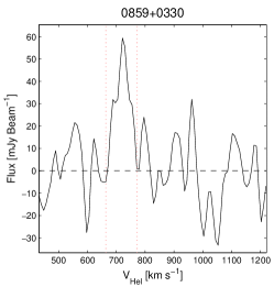
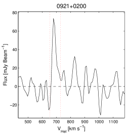
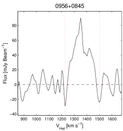
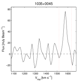
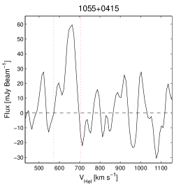
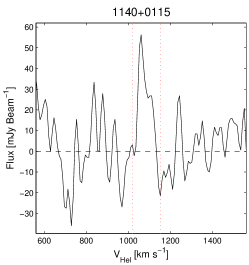
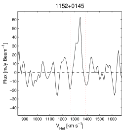
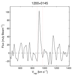
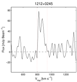
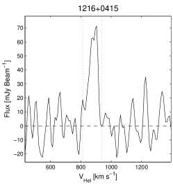
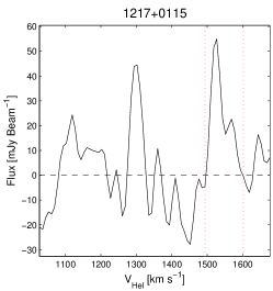
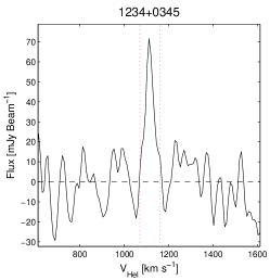
Figure 7: H i spectra of the new detections in the Westerbork Virgo Filament Survey at the position of the highest peak flux. The velocity interval over which the integrated line strength has been determined is indicated by the two vertical dashed lines.

Fig 7. (continued)

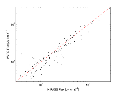
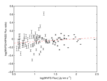
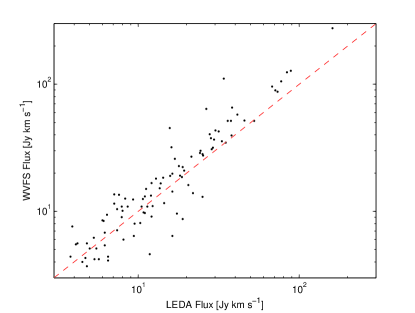
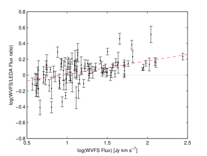
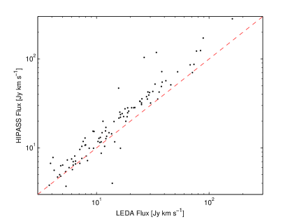
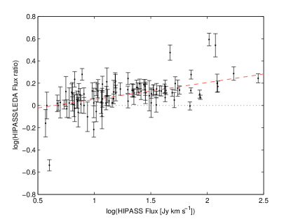
Figure 8: Comparison of determined H i fluxes with values obtained from HIPASS and LEDA. The left panels show the direct relation between the different catalogues, with the red line indicating the points where fluxes are equivalent. The right panels show the ratio between two catalogues as function of flux, both on a logarithmic scale, the red line indicated here the best power law fit through the data points. The first row shows the comparison between WVFS and HIPASS fluxes, while the second row shows the comparison between WVFS and LEDA. As a reference, the comparison between HIPASS and LEDA fluxes is plotted in the bottom row.

4.5 H i in the extended galaxy environment

We compare our measured galaxy fluxes with the fluxes measured by the H i Parkes all sky survey (HIPASS) and fluxes tabulated in LEDA. Only those sources are considered for which the integrated signal-to-noise ratio is larger than 8 in both the WVFS and HIPASS surveys. Furthermore, galaxies have been excluded which occur at the edge of the WVFS band, as no complete spectrum can be derived for these sources, resulting in an integrated flux value that is known to be only a lower limit.

It is interesting to look for any systematic differences in total flux between the several catalogues. Flux values derived from both WVFS and HIPASS have undergone a uniform calibration procedure that was similar for all sources. Both surveys are single dish surveys with a relative large primary beam sizes of 15’ for HIPASS and 49’ for WVFS after spatial smoothing. At a distance of 10 Mpc, these beam sizes correspond to 40 and 140 kpc respectively, comparable to or larger than the typical H i diameter of a galaxy.

The LEDA fluxes are compiled from measurements made with very different telescopes, yielding much greater variety in calibration procedures. Because the fluxes are obtained from different telescopes, it is not possible to relate the fluxes to one specific beam size.

In the left panels of Fig. 8 the integrated flux values of the three catalogues are compared, with WVFS vs. HIPASS in the top panel, WVFS vs. LEDA in the middle panel and HIPASS vs. LEDA in the bottom panel. The dashed line goes through the origin of the diagram, with a slope of one, indicating identical fluxes. The best correspondence is between the HIPASS and WVFS data as the points are scattered around the red line. When looking at the WVFS-LEDA comparison, there is agreement for fluxes below $\sim 20$ Jy km s^-1, but for larger fluxes all WVFS fluxes seem to be systematically higher. The same effect is apparent in the HIPASS-LEDA comparison.

To have a better understanding of the differences, the flux ratios of the different catalogue pairs are plotted in the right panel. Fluxes and flux ratios are both plotted on a logarithmic scale, equivalent flux values are indicated by the black dotted line at zero. The data points in each plot are fitted with a power law function, indicated by the dashed line.

The scatter in the WVFS-HIPASS comparison is almost perfectly centered around zero. The fitted power law has a slope of $a=0.069\pm 0.07$ and a scaling factor of $b=-0.14\pm 0.09$. There is one source which is significantly stronger in the WVFS data, which is WVFS 1210+0300 or UGC 7185. The reason for this large discrepancy is not clear. There are quite a few sources for which the measured flux in HIPASS is significantly higher. This can be partially ascribed to confusion effects, as has been described earlier.

The flux ratios between WVFS and LEDA show substantial deviations especially for larger flux values. The power law fit has a relatively steep slope of $a=0.15\pm 0.05$ and a scaling factor of $b=-0.1\pm 0.08$. Above a 20 Jy km s^-1 flux limit, the WVFS values are brighter than the LEDA values without any exception.

Because this is quite a dramatic result, the same comparison has been done between the HIPASS and LEDA fluxes in the bottom right panel of Fig. 8. Although the power law fit has a very similar slope compared to the WVFS data of $a=0.16\pm 0.05$, the scaling factor of $b=-0.15\pm 0.08$ is marginally larger.

The general conclusion is that both WVFS and HIPASS find significantly more H i in galaxies than LEDA. This effect is strongest for objects with an H i flux above 20 Jy km s^-1. Above this level the excess in H i flux for both these single dish surveys is $\sim 40$%.

A possible explanation is that both HIPASS and WVFS are more sensitive to diffuse emission, due to the large intrinsic beam sizes. The flux values listed by LEDA, are based on a combination of fluxes obtained in different measurements. Although we cannot access these individual values, a large number of the flux values were likely obtained with smaller intrinsic beam sizes, e.g. interferometric data. In general, a smaller intrinsic beam is much less sensitive to diffuse emission than a large beam, and therefore will miss diffuse emission preferentially. However, the differences between WVFS and LEDA are remarkably large and systematic which is a point of concern. For some individual targets we have compared the flux values of LEDA with all available flux values given by the NASA Extragalactic Database (NED). Here we find a similar trend: flux values listed in NED are generally much higher than the values given by LEDA. To derive H i fluxes, the LEDA team do not merely calculate a weighted average of available flux values from the literature. Several corrections are applied in an attempt to get more uniformity among the fluxes, and the result is then scaled to fluxes obtained with the Nancay telescope.

We have confidence in the calibration of the WVFS data and the derived fluxes of our detections and see excellent correspondence with the HIPASS catalog. We have serious reservations regarding the accuracy of the LEDA-tabulated H i fluxes.

4.6 Line width and Gas accretion modes

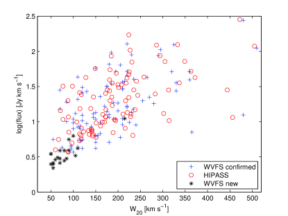
Figure 9: Flux as function of $W_{20}$ for the WVFS detections and the same detection in HIPASS. The behaviour of HIPASS and WVFS detections agree very well, in general objects with a larger flux have a broader line-width.

In Fig. 9 the flux of each detection is plotted as function of $W_{20}$, the line-width at 20% of the peak. Known and confirmed detections are shown with blue plus signs, while the new detections are plotted as black stars, the known detections are compared with the same objects from the HIPASS database, shown as red circles. The same basic trend is apparent in both the HIPASS and WVFS tabulations, with brighter detections generally accompanied by a larger line-width. The new WVFS detections simply extend this trend to low brightnesses and the lowest line-widths.

By measuring the line-widths of the detections, an estimate can be given of the upper limit of the kinetic temperature, using the equation:

$$T_{kin}\leq\frac{m_{H}\Delta v^{2}}{8k_{B}\textrm{ln}2}$$ (5)

where $m_{H}$ is the mass of an hydrogen atom, $k_{B}$ is the Boltzmann constant and $\Delta v$ is the FWHM H i line-width. Apart from one detection with a velocity width of 215 km s^-1, the velocity widths of all the detections are between 50 and 110 km s^-1. When assuming that the lines are not broadened by internal turbulence or rotation, the maximum temperatures range between $\sim 5\cdot 10^{4}$ and $\sim 3\cdot 10^{5}$ K. If the new detections without an optical counterpart are indeed related to the cosmic web, then this gas could be examples of the cold accretion mode as described in Kereš et al. (2005), where gas is directly accreting from the intergalactic medium onto the galaxies at temperatures of $\sim 10^{5}$ K, without being shock-heated to very high temperatures. We note that the neutral fraction of gas is expected to drop very rapidly for temperatures above $10^{5}$ K and hence it is very unlikely that high H i column densities would be associated with thermally dominated linewidths greatly exceeding 100 km s^-1.

4.7 Non Detections

The H i Parkes All Sky Survey completely covers the region observed in the WVFS. In this region a total of 147 objects are listed in the HIPASS catalogue within the velocity coverage of WVFS. Most of these sources could be detected and confirmed by the WVFS, although some of them could not be identified individually, due to confusion. For three sources listed in HIPASS we could not determine H i emission in the WVFS.

NGC 4457 has a flux of 7.2 Jy km s^-1 in HIPASS and 4.4 Jy km s^-1 is listed in the LEDA database. Although there is substantial discrepancy between those numbers, the source has significant flux and should be easily detected in the WVFS. There is a tentative detection in the WVFS data at the expected position and velocity, however it does not pass our detection limit.

HIPASS J1233-00 has a flux of 3.0 Jy km s^-1 in HIPASS and 2.9 Jy km s^-1 in LEDA. Although these numbers are consistent, it is a weak detection, especially when taking into account the $W_{20}$ value of 112 km s^-1 listed in the HIPASS catalogue. The source does not appear in WVFS, but it would be near the detection limit.

HIPASS J1515+05 has a flux of 2.5 km s^-1 in HIPASS with a $W_{20}$ value of 121 km s^-1, making this a very weak detection. The integrated line strength has a signal-to-noise value of only 4, when taking into account the sensitivity of HIPASS. There is no indication for H i in the WVFS, but also none in the LEDA and NED databases.

Since we only expect a source completeness level of about 90% at our 8$\sigma$ significance threshold (Corbelli & Bandiera (2002)) it is not surprising that several faint cataloged sources are not redetected independently in the WVFS.

5 Discussion and Conclusion

We have carried out an unbiased wide-field H i survey of $\sim 1300$ deg² of sky, mapping the galaxy filament connecting the Local Group with the Virgo cluster. In the total power data we are especially sensitive to very diffuse and extended emission, due to the large intrinsic beam size of the observation. Apart from three sources, we can confirm all detections that have been obtained with the H i Parkes All Sky Survey in this region, when taking into account confusion effects. Apart from previously known sources, we identify 20 new candidate detections with an integrated H i flux exceeding 8$\sigma$. These candidates have a typical integrated column density of only $\sim 3\times 10^{17}$ cm^-2, when assuming that the emission is filling the beam. The velocity width at 20% of the peak ranges between $\sim 50$ and $\sim 100$ km s^-1 with the exception of one object with a significantly broader line width of 215 km s^-1.

If these candidates are intrinsically diffuse structures, then they could not have been detected in HIPASS or any other currently available wide-field H i survey, as the WVFS column density sensitivity is about an order of magnitude better. The objects would be at the one sigma level in the full resolution HIPASS data, which makes identification extremely difficult, even assuming that spatial smoothing were applied after-the-fact.

For most of our new candidates we can not find a clear optical counterpart, making direct confirmation difficult. As our data is so sensitive, we are exploring a new realm in detecting very diffuse and extended H i and there is not much data available in the literature to compare with. The detection limits have been set fairly conservatively in that the integrated flux has to exceed a signal-to-noise of 8. In addition, we only accept candidates that are individually apparent in both the rise and set data, which are two independent observations.

The new candidate detections have properties similar to the H i filament connecting M31 and M33, as described in Braun & Thilker (2004). This filament has a very comparable column density to the WVFS detections of $3\times 10^{17}$ cm^-2 without a clearly identified optical counterpart.

Follow up observations, at higher resolution but with similar brightness sensitivity are critical. This can not only confirm the detections, but also put more constraints on the actual peak column densities. A possible scenario might be that our candidate detections are actually collections of discrete bright clumps, the flux of which is diluted in our large beam. This is unlikely, as in that case the clumps should have been detected individually by HIPASS, which achieves a slightly better point source sensitivity than the WVFS.

If these candidates and their low intrinsic column densities can be confirmed, we can for the first time identify a whole class of objects related to filaments of the Cosmic Web; very extended gas clouds with extremely low neutral column densities in the intergalactic medium.

The original HIPASS data and the WVFS cross-correlation data will serve as follow-up observations for the sample presented here. Although the brightness sensitivity of both these surveys is not as good as for the WVFS total power data, gas clumps with slightly higher column densities can be easily identified. As mentioned previously, the comparison with these surveys and detailed analysis will be explained in forthcoming papers. With all three survey coverages in hand, the data can be interpreted more effectively. We hope to confirm several of the intergalactic H i detections and put more light on the intergalactic reservoir of gas in the vicinity of galaxies. By looking at the kinematics and line widths of the detections, we hope to learn more about galaxy and AGN feedback and whether galaxies are fueled preferentially through hot-mode or cold-mode accretion processes.

Appendix A Spectra of confirmed H i detections in the WVFS total power data.

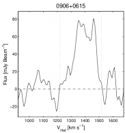
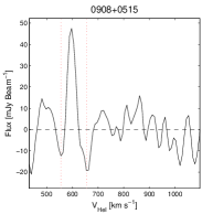
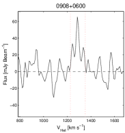
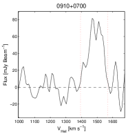
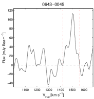
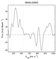
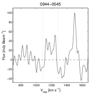
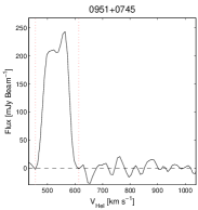
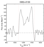
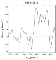
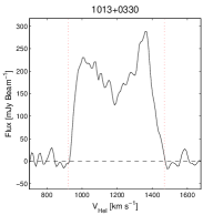
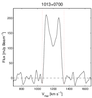
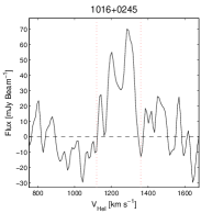
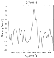
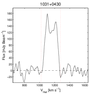
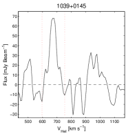
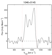
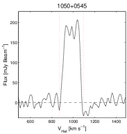
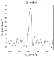
Figure 10: Spectra of all detections of neutral hydrogen in the WVFS total power data. The velocity width of each object is indicated by the two vertical dotted lines.

Fig 10. (continued)

Fig 10. (continued)

Fig 10. (continued)

Fig 10. (continued)

Fig 10. (continued)

Fig 10. (continued)