Real stabilization of resonance states employing two parameters: basis set size and coordinate scaling

Abstract

The resonance states of one- and two-particle Hamiltonians are studied using variational expansions with real basis-set functions. The resonance energies, $E_{r}$, and widths, $\Gamma$, are calculated using the density of states and an ${\mathcal{L}}^{2}$ golden rule-like formula. We present a recipe to select adequately some solutions of the variational problem. The set of approximate energies obtained shows a very regular behaviour with the basis-set size, $N$. Indeed, these particular variational eigenvalues show a quite simple scaling behaviour and convergence when $N\rightarrow\infty$. Following the same prescription to choose particular solutions of the variational problem we obtain a set of approximate widths. Using the scaling function that characterizes the behaviour of the approximate energies as a guide, it is possible to find a very good approximation to the actual value of the resonance width.

I Introduction

The methods used to calculate the energy and the lifetime of a resonance state are numerous moisereport ; reinhardt1996 ; sajeev2008 ; bylicki2005 ; dubau1998 ; kruppa1999 ; kar2004 and, in some cases, has been put forward over strong foundations simon78 . However, the analysis of the numerical results of a particular method when applied to a given problem is far from direct. The complex scaling (complex dilatation) method moisereport , when the Hamiltonian $H$ allows its use, reveals a resonance state by the appearance of an isolated complex eigenvalue on the spectrum of the non-Hermitian complex scaled Hamiltonian, $H(\theta)$ moisereport . Of course in an actual implementation the rotation angle $\theta$ must be large enough to rotate the continuum part of the spectrum beyond the resonance’s complex eigenvalue. Moreover, since most calculations are performed using finite variational expansions it is necessary to study the numerical data to decide which result is the most accurate. To worsen things the variational basis sets usually depend on one (or more) non-linear parameter. For bound states the non-linear parameter is chosen in order to obtain the lowest variational eigenvalue. For resonance states things are not so simple since they are embedded in the continuum. The complex virial theorem together with some graphical methods moiseyev1981 ; moiseyev1980 allows to pick the best numerical solution of a given problem, which corresponds to the stabilized points in the $\theta$ trajectories moisereport ; moiseyev1981 ; moiseyev1980 .

Other methods to calculate the energy and lifetime of the resonance, based on the numerical solution of complex Hamiltonians, also have to deal with the problem of which solutions (complex eigenvalues) are physically acceptable. For example, the popular complex absorbing potential method, which in many cases is easier to implement than the complex scaling method, produces the appearance of nonphysical complex energy stabilized points that must be removed in order to obtain only the physical resonances sajeev2009 .

The aforementioned issues explain, at some extent, why the methods based only in the use of real ${\mathcal{L}}^{2}$ variational functions are often preferred to analyze resonance states. These techniques reduce the problem to the calculation of eigenvalues of real symmetric matrices kar2004 ; pont2010 ; pont2010b ; kar2007 ; kar2007b ; kruppa1999 . Of course, these methods also have its own drawbacks. One of the main problems was recognized very early on (see, for example, the work by Hol$\phi$ien and Midtdal holfien1966 ): if the energy of an autoionizing state is obtained as an eigenvalue of a finite Hamiltonian matrix, which are the convergence properties of these eigenvalues that lie in the continuum when the size of the Hamiltonian matrix changes? But in order to obtain resonance-state energies it is possible to focus the analysis in a global property of the variational spectrum: the density of states (DOS)mandelshtam1993 , being unnecessary to answer this question.

The availability of the DOS allows to obtain the energy and lifetime of the resonance in a simple way, both quantities are obtained as least square fitting parameters, see for example kar2007 ; kruppa1999 . Despite its simplicity, the determination of the resonance’s energy and width based in the DOS is far from complete. There is no a single procedure to asses both, the accuracy of the numerical findings and its convergence properties, or which values to pick between the several “candidates” that the method offers kar2004 .

Recently, Pont et al pont2010b have used finite size scaling arguments ks2003 to analyze the properties of the DOS when the size of the Hamiltonian changes. They presented numerical evidence about the critical behavior of the density of states in the region where a given Hamiltonian has resonances. The critical behavior was signaled by a strong dependence of some features of the density of states with the basis-set size used to calculate it. The resonance energy and lifetime were obtained using the scaling properties of the density of states. However, the feasibility of the method to calculate the resonance lifetime laid on the availability of a known value of the lifetime, making the whole method dependent on results not provided by itself.

The DOS method relies on the possibility to calculate the Ritz-variational eigenfunctions and eigenvalues for many different values of the non-linear parameter $\eta$ (see Kar and Ho  kar2004 ). For each basis-set size, $N$, used, there are $N$ variational eigenvalues $E_{N}^{m}(\eta);\;m=1,\ldots,N$. Each one of these eigenvalues can be used, at least in principle, to compute a DOS, $\rho_{N}^{m}(E)$, resulting, each one of these DOS in an approximate value for the energy, $E_{r}\sim E_{N}^{m}$, and width, $\Gamma\sim\Gamma_{N}^{m}$, of the resonance state of the problem. If the variational problem is solved for many different basis-set sizes, there is not a clear cut criterion to pick the “better” result from the plethora of possible values obtained. This issue will be addressed in Section III.

In this work, in order to obtain resonance energies and lifetimes, we calculate all the eigenvalues for different basis-set sizes, and present a recipe to select adequately certain values of $N$, and one eigenvalue for each $N$ elected, that is, we get a series of variational eigenvalues $\{E_{N_{i}}^{m_{i}}(\eta)\}$.

The recipe is based on some properties of the variational spectrum which are discussed in Section II. The properties seem to be fairly general, making the implementation of the recipe feasible for problems with several particles. Actually, because we use scaling properties for large values of $N$, the applicability of the method for systems with more than three particles could be restricted because the difficulties to handle large basis sets.

The set of approximate resonance energies, obtained from the density of states of a series of eigenvalues selected following the recipe, shows a very regular behaviour with the basis set size. This regular behaviour facilitates the use of finite size scaling arguments to analyze the results obtained, in particular the extrapolation of the data when $N\longrightarrow\infty$. The extrapolated values are the most accurate approximation for the parameters of the resonance state that we obtain with our method. This is the subject of Section IV, where we present results for models of one and two particles.

Following the same prescription to choose particular solutions of the variational problem we obtain a set of approximate widths in Section V. Using the scaling function that characterizes the behaviour of the approximate energies as a guide, it is possible to find a very good approximation to the resonance width since, again, the data generated using our prescription seems to converge when $N\rightarrow\infty$. Finally, in Section VI we summarize and discuss our results.

II Some properties of the variational spectrum

When one is dealing with the variational spectrum in the continuum region, some of its properties are not exploited to obtain more information about the presence of resonances, usually the focus of interest is the stabilization of the individual eigenvalues. The stabilization is achieved varying some non-linear variational parameter. If $\eta$ is the inverse characteristic decaying length of the variational basis functions, then the spectrum of the kinetic energy scales as $\eta^{2}$, moreover, for potentials that decay fast enough, the spectrum of the whole Hamiltonian also scales as $\eta^{2}$ for large (or small) enough values of $\eta$ (see appendix). This is so, since the variational eigenfunctions are ${\mathcal{L}}^{2}$ approximations to plane waves except when $\eta$ belongs to the stabilization region. When $\eta$ belong to the stabilization region of a given variational eigenvalue, say $E_{N}^{m}(\eta)$, then $E_{N}^{m}(\eta)\sim E_{r}$ (where $E_{r}$ is the resonance energy) and the variational eigenfunction $\psi_{N}^{m}(\eta)$ has the localization length of the potential well. We intend to take advantage of the changes of the spectrum when $\eta$ goes from small to large enough values.

The variational spectrum satisfies the Hylleras-Undheim theorem or variational theorem: if $N$ is the basis set size, and $E_{N}^{m}$ is the $m-th$ eigenvalue obtained with a variational basis set of size $N$, then

$$E_{N}^{m}(\eta)\geq E_{N+1}^{m}(\eta).$$

Actually, since the threshold of the continuum is an accumulation point, then for small enough values of $\eta$ and a given $j\in\mathbb{N}$ there is always a $k\in\mathbb{N}$ such that

$$E_{N}^{m}(\eta_{small})>E_{N+k}^{m+j}(\eta_{small}).$$ (1)

For the kinetic energy variational eigenvalues, and for fixed $N,m,j$, and $k$, if the ordering given by Equation (1) holds for some $\eta$ then it is true for all $\eta$. Of course this is not true for a Hamiltonian with a non zero potential that support resonance states. So, we will take advantage of the variational eigenvalues such that for $\eta$ small enough satisfies Equation (1) but, for $\eta$ large enough

$$E_{N}^{m}(\eta_{large})<E_{N+k}^{m+j}(\eta_{large}).$$ (2)

Despite its simplicity, the arguments above give a complete prescription to pick a set of eigenstates that are particularly affected by the presence of a resonance. Choose $N$ and $m$ arbitrary, and then look for the smaller values of $j$ and $k$ such that the two inequalities, Equations. (1) and (2) are fulfilled. So far, all the examples analyzed by us show that if the inequalities are satisfied for some $j$ and $k$ then they are satisfied too by the eigenvalues $E_{N+nk}^{m+nj}$, for $n=2,3,4,\ldots$.

III Models and methods

To illustrate how our prescription works we used two different model Hamiltonians. The first model, due to Hellmann hellman35 , is a one particle Hamiltonian that models a $N_{e}$-electron atom. The second one is a two particle model that has been used to study the low energy and resonance states of two electrons confined in a semiconductor quantum dot pont2010b .

The details of the variational treatment of both models will be kept as concise as possible. The one particle model has been used before for the determination of critical nuclear charges for $N_{e}$-electron atoms sergeev1999 , it also gives reasonable results for resonance states in atomic anions sabre2001 and continuum states  colavecchia2009 . The interaction of a valence electron with the atomic core is modeled by a one-particle potential with two asymptotic behaviours. The potential behaves correctly in the regions where electron is far from the atomic core ($N_{e}-1$ electrons and the nucleus of charge $Z$) and when it is near the nucleus. The Hamiltonian, in scaled coordinates $r\rightarrow Z\,r$, is

$$H=-\frac{1}{2}\nabla^{2}-\frac{1}{r}+\frac{\gamma}{r}\left(1-e^{-\delta r}\right),$$ (3)

where $\gamma=\left(\frac{N_{e}-1}{Z}\right)$ and $\delta$ is a range parameter that determines the transition between the asymptotic regimes, for distances near the nucleus $V_{0}(r)\approx-\frac{1}{r}$ and in the case $r\rightarrow\infty$ the nucleus charge is screened by the $N_{e}-1$ localized electrons and $V_{\infty}(r)\approx-\frac{Z-N_{e}+1}{Zr}$.

Another advantage of the potential comes from its analytical properties. In particular this potential is well behaved and the energy of the resonance states can be calculated using complex scaling methods. So, besides its simplicity, the model potential allows us to obtain the energy of the resonance by two independent methods and check our results.

The two particle model that we considered describes two electrons interacting via the Coulomb repulsion and confined by an external potential with spherical symmetry. We use a short-range potential suitable to apply the complex scaling method. The Hamiltonian $H$ for the system is given by

$$H=-\frac{\hbar^{2}}{2m}\nabla_{{\mathbf{r}}_{1}}^{2}-\frac{\hbar^{2}}{2m}\nabla_{{\mathbf{r}}_{2}}^{2}+V(r_{1})+V(r_{2})+\frac{e^{2}}{\left|{\mathbf{r}}_{2}-{\mathbf{r}}_{1}\right|},$$ (4)

where $V(r)=-(V_{0}/r_{0}^{2})\,\exp{(-r/r_{0})}$, ${\mathbf{r}}_{i}$ the position operator of electron $i=1,2$; $r_{0}$ and $V_{0}$ determine the range and depth of the dot potential. After re-scaling with $r_{0}$, in atomic units, the Hamiltonian of Equation (4) can be written as

$$H=-\frac{1}{2}\nabla_{{\mathbf{r}}_{1}}^{2}-\frac{1}{2}\nabla_{{\mathbf{r}}_{2}}^{2}-V_{0}e^{-r_{1}}-V_{0}e^{-r_{2}}+\frac{\lambda}{\left|{\mathbf{r}}_{2}-{\mathbf{r}}_{1}\right|},$$ (5)

where $\lambda=r_{0}$.

The variational spectrum of the two particle model, Equation (5), and all the necessary algebraic details to obtain it, has been studied with great detail in Reference pont2010b so, until the end of this Section, we discuss the variational solution of the one particle model given by Equation (3).

The discrete spectrum and the resonance states of the model given by Equation (3) can be obtained approximately using a real ${\cal L}^{2}$ truncated basis set $\left\{\Phi_{i}(\eta)\right\}_{1}^{N}$ to construct a $N\times N$ Hamiltonian matrix $H_{ij}(\eta)=\left\langle\Phi_{i}(\eta)\right|H\left|\Phi_{j}(\eta)\right\rangle$. We use the Rayleigh-Ritz Variational method to obtain the approximations $\left|\psi_{N}^{m}(\eta)\right\rangle$

$$\left|\psi_{N}^{m}(\eta)\right\rangle\,=\,\sum_{i=1}^{N}c^{(m)}_{i}(\eta)\left|\Phi_{i}(\eta)\right\rangle\,,\;\;\;\;\;\;m=1,\cdots,N\,.$$ (6)

For bound states this functions are variationally optimal. The functions $\left|\Phi_{i}(\eta)\right\rangle$ are

$$\left|\Phi_{i}(\eta)\right\rangle=\frac{\eta^{3/2}e^{-\eta r/2}}{\sqrt{(i+1)(i+2)}}L^{(2)}_{i}(\eta r)$$ (7)

and $L^{(2)}_{i}(\eta r)$ are the associated Laguerre polynomials of $2^{\textrm{nd}}$ order and degree $i$. The non-linear parameter $\eta$ is used for eigenvalue stabilization in resonance analysis kar2004 ; kar2007 ; kar2007b . Note that $\eta$ plays a similar role that the finite size of the box in spherical box stabilization procedures cederbaum80 , as stated by Kar et. al. kar2004 .

Resonance states are characterized by isolated complex eigenvalues, $E_{res}=E_{r}-i\Gamma/2,\;\Gamma>0$, whose eigenfunctions are not square-integrable. These states are considered as quasi-bound states of energy $E_{r}$ and inverse lifetime $\Gamma$. For the Hamiltonian Equation (3), the resonance energies belong to the positive energy range reinhardt1996 .

Using the approximate solutions of Hamiltonian (3) we analyze the DOS method mandelshtam1993 that has been used extensively to calculate the energy and lifetime of resonance states, in particular we intend to show that 1) the DOS method provides a host of approximate values whose accuracy is hard to assess, and 2) if the DOS method is supplemented by a new optimization rule, it results in a convergent series of approximate values for the energy and lifetime of resonance states.

The DOS method

The DOS method relies on the possibility to calculate the Ritz-variational eigenfunctions and eigenvalues for many different values of the non-linear parameter $\eta$ (see Kar and Ho  kar2004 ).

The localized DOS $\rho(E)$ can be expressed as mandelshtam1993

$$\rho(E)=\left|\frac{\partial E(\eta;\gamma,\delta)}{\partial\eta}\right|^{-1}.$$ (8)

Since we are dealing with a numerical approximation, we calculate the energies in a discretization $\left\{\eta_{i}\right\}$ of the continuous parameter $\eta$. In this approximation, Equation (8) can be written as

$$\rho_{N}^{m}(E)=\rho(E_{N}^{m}(\eta_{i};\gamma,\delta))=\left|\frac{E_{N}^{m}(\eta_{i+1};\gamma,\delta)-E_{N}^{m}(\eta_{i-1};\gamma,\delta)}{\eta_{i+1}-\eta_{i-1}}\right|^{-1}$$ (9)

where $E_{N}^{m}(\eta;\gamma,\delta)$ is the $j$-th eigenvalue of the $N\times N$ matrix Hamiltonian with $\gamma$ and $\delta$ fixed.

In complex scaling methods the Hamiltonian is dilated by a complex factor $\alpha=|\alpha|\,e^{-i\theta}$. As was pointed out long time ago by Moiseyev and coworkers moiseyev79 , the role played by $\eta$ and $|\alpha|$ are equivalent, in fact, our parameter $\eta$ corresponds to $\alpha(\theta=0)$. Besides, the DOS attains its maximum at optimal values of $\eta$ and $E_{r}$ that could be obtained with a self-adjoint Hamiltonian without using complex scaling methods moiseyev1980 . So, locating the position of the resonance using the maximum of the DOS is equivalent to the stabilization criterion used in complex dilation methods that requires the approximate fulfillment of the complex virial theorem moiseyev1981 .

The values of $E_{r}(\gamma,\delta)$ and $\Gamma(\gamma,\delta)$ are obtained performing a nonlinear fitting of $\rho(E)$, with a Lorentzian function,

$$\rho(E)=\rho_{0}+\frac{A}{\pi}\frac{\Gamma/2}{\left[(E-E_{r})^{2}+(\Gamma/2)^{2}\right]}.$$ (10)

One of the drawbacks of this method results evident: for each pair $\gamma,\delta$ there are several $\rho_{N}^{m}(E)$, and since each $\rho_{N}^{m}(E)$ provides a value for $E_{r}(N,m)$ and $\Gamma(N,m)$ one has to choose which one is the best. Kar and Ho kar2004 solve this problem fitting all the $\rho_{N}^{m}(E)$ and keeping as the best values for $E_{r}$ and $\Gamma$ the fitting parameters with the smaller $\chi^{2}$ value. At least for their data the best fitting (the smaller $\chi^{2}$) usually corresponds to the larger $j$. This fact has a clear interpretation, if the numerical method approximates $E_{r}$ with some $E_{r}(N,j)$, where $N$ is the basis set size of the variational method, a large $j$ means that the numerical method is able to provide a large number of approximate levels, and so the continuum of positive-energy states is “better” approximated.

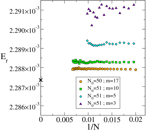
Figure 1: (color on-line) $E_{r}(N,m)$ vs $1/N$ for $(\gamma=1.125,\delta=0.211)$. The values were obtained from the peak of the DOS resulting from Equation (9) for several basis set sizes, $N=N_{0}+3\,k;\;k=0,\ldots,k_{m}$. The (orange) dots data correspond to $N_{0}=50$ $m=17$ and $k_{m}=33$; the (green) square dots to $N_{0}=51$, $m=10$ and $k_{m}=32$; the (cyan) diamond dots to $N_{0}=51$ $m=5$ and $k_{m}=17$; and the (violet) triangle dots to $N_{0}=51$ $m=3$ and $k_{m}=17$. The cross shows the value we obtained using complex scaling $(\theta=\pi/5,N=70)$.

In a previous work pont2010b we have shown that a very good approximation to the energy of the resonance state is obtained considering just the energy value where $\rho_{N}^{m}(E)$ attains its maximum. We denote this value as $E_{r}(N,m)$. Figure 1 shows the approximate resonance energy $E_{r}(N,m)$ for different basis set size $N$, where $m$ is the index of the variational eigenvalue used to calculate the DOS. We used the values $\gamma=1.125$ and $\delta=0.211$ corresponding to the ones used before sabre2001 in the analysis of $O^{--}$ resonances. The Figure 1 also shows the value calculated using complex scaling. It is clear that the accuracy of all the values shown is rather good (all the values shown differ in less than 6$\times 10^{-6}$), and that larger values on $n$ provide better values for the resonance energy. These facts are well known from previous works, i.e. almost all methods to calculate the energy of the resonance give rather stable and accurate results for $E_{r}$. However, the practical importance of this fact is reduced: these are uncontrolled methods, so the accuracy of the values obtained from the DOS can not be assessed (without a value independently obtained) and these values do not seem to converge to the value obtained using complex scaling when $N$ is increased and $n$ is kept fixed.

There is another fact that potentially could render the whole method useless: for small or even moderate $m$, the values $E_{r}(N,m)$ become unstable (see Figure 1) when $N$ is large enough. This last point has been pointed previously holfien1966 . In the problem that we are considering is rather easy to obtain a large number of variational eigenvalues in the interval where the resonances are located, allowing us to calculate $E_{r}(N,m)$ up to $m=17$, but this situation is far from common see, for example, References pont2010 ; pont2010b ; ferron2009 .

IV Scaling of the resonance energy

So far we have presented only results about the behaviour of the one particle Hamiltonian, from now on we will discuss both models, Equations (3) and 5.

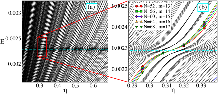
Figure 2: (color on-line) (a) Variational spectrum obtained for several basis set sizes of the one-particle Hamiltonian. There are two noticeable features associated to changes in the the density of curves. One of these features corresponds to the stabilization zone, where the derivative of the eigenvalues is minimal and, correspondingly, the density of states is larger. The other one corresponds to the gaps in the density of eigenvalues when $E$ is kept fixed. (b) Detailed view of the data shown in panel (a). There is a well defined crossing between several eigenvalues, which form a bundle of states. The bundle is formed by $E_{52}^{13},E_{56}^{14},E_{60}^{15},E_{64}^{16}$, and $E_{68}^{17}$.

It is known that the variational eigenvalues $E_{N}^{m}(\eta)$ do not present crossings when they are calculated for some fixed values of $N$, i.e the variational spectrum is non-degenerate for any finite Hamiltonian matrix. As a matter of fact the avoided crossings between successive eigenvalues in the variational spectrum are the watermark of a resonance. An interesting feature emerges when the variational spectrum for many different basis set sizes $N$ are plotted together versus the parameter $\eta$. Besides the places where $\frac{dE_{N}^{m}(\eta)}{d\eta}$ attains its minimum value, which correspond to the stabilization points, there are some gaps which correspond to crossings between eigenvalues obtained with different basis set sizes, see Figure 2. Moreover, the crossings corresponds to eigenvalues with different index $m$, and are the states that satisfy the inequalities Equations (1),and (2).

It is worth to remark that the main features shown by Figure 2 are independent of the number of particles of the Hamiltonian and the particular values of the threshold of the continuum. Figure 3 shows the behaviour of the variational eigenvalues obtained for the two particle Hamiltonian Equation (5). In this case the ionization threshold is not the asymptotic value of the potential, but it is given by the energy of the one particle ground state. The resonance state came from the two-particle ground state that becomes unstable and enters into the continuum of states when the quantum dots becomes “too small” to accommodate two electrons. For more details about the model, see reference pont2010b .

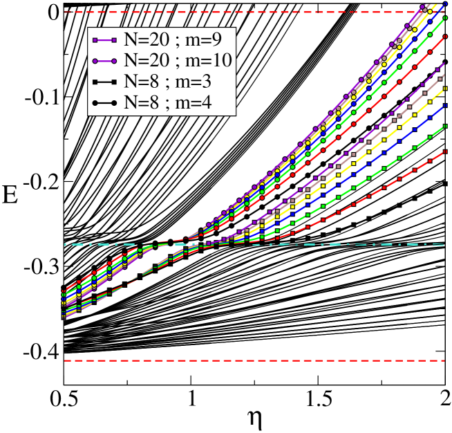
Figure 3: (color on-line) Rayleigh-Ritz energies as a function of the nonlinear parameter $\eta$. The calculations are for the resonances of the two-electron quantum dot model used in pont2010b . The Energies are calculated for $V_{0}=3$ and $\lambda=1.1$ of equation (5). The dot and squares denote two different bundles both calculated with basis-set sizes $N_{0}=8;\;\Delta N=2$. The eigenvalue numbers for the dotted bundle are given by $m_{0}=4;\;\Delta m=1$. For the bundle with squares the values are $m_{0}=3;\;\Delta m=1$. The eigenvalues corresponding to the minimum ($N=8$) and maximum ($N=20$) basis-set size are single out. The dash-dotted cyan line is the resonance energy calculated using complex scaling. The dashed red lines indicates the exact energies where the continuum begins.

The left panel of Figure 4 shows the behaviour of the maximum value of the DOS, $\rho_{max}^{-1}(N,m)$, for the one particle Hamiltonian, obtained for different basis-set sizes and fixed $m$ (in this case $m=17$), and the $\rho_{max}(N,m)$ obtained choosing a “bundle” of states that are linked by a crossing, these states have $N=51,54,57,\ldots,168$ and $m=16,17,18,\ldots,55$ respectively. From our numerical data, the maximum value of the DOS scales with the basis-set size following two different prescriptions. For $m$ fixed, $\rho_{max}(N,m)\sim N^{\alpha}$, with $\alpha>0$, while when the pair $(N,m)$ is chosen from the set of pairs that label a bundle of states $\rho_{max}(N,m)\sim N^{-\beta}$, with $\beta>0$. In particular, for $m=17$ we get that $\rho_{max}(N,17)\sim N^{0.759}$, and $\rho_{max}(N,m)\sim N^{-1}$ when $(N,m)=(51,17),(54,18),(57,19),\ldots$.

Figure 4: . (a) Scaling of the DOS peak vs. the inverse basis-set size $N$. One particle Hamiltonian. The figure shows the peak values with increasing $N=51,54,57,\ldots,168\,$, for $m=17$ fixed (red crosses). The peaks for a bundle of eigenvalues ($N_{0}=51;\;\Delta N=3;\;m_{0}=17;\;\Delta m=1$) show a linear scaling (black dots). For series of states that form bundles not associated to a crossing the scaling with $1/N$ is greater ( $N_{0}=51;\,\Delta N=3\,;\,m_{0}=16\,;\,\Delta m=1$, green triangle up dots) or lower ($N_{0}=51;\,\Delta N=3\,;\,m_{0}=18\,;\,\Delta m=1$, orange triangle down dots) than $1$. (b) The energy position of the DOS peaks as a function of $1/N$. The figure shows that the fixed $m=17$ resonance energies (red crosses) do not converge to the resonance energy calculated by complex scaling (bold black cross). The scaling for the bundle, and near bundle, series of states is almost linear and an extrapolated value can be estimated.

Of course we can pick sets of states that are not related by a crossing. For instance, we also picked sets with a simple prescription as follows: choose a given initial pair $(N_{0},m_{0})$ and form a set of states with the states labeled by $(N_{0},m_{0}),(N_{0}+\Delta N,m_{0}+\Delta m),(N_{0}+2\Delta N,m_{0}+2\Delta m)$ and so on. Figure 4(a) shows two examples obtained choosing $N_{0}=51$, $\Delta N=3$ and $m_{0}=16$ and $m_{0}=18$ both with $\Delta m=1$. Quite interestingly, the data in Figure 4 show that the scaled maxima of the DOS for a bundle and two different sets seem to converge to the same value when $N\rightarrow\infty$, but only for the bundle the scaling function is $N^{-1}$. The advantage obtained from picking those eigenvalues $E_{N}^{m}(\eta)$ that belong to a given bundle is still more evident when the corresponding DOS and $E_{r}$ are calculated. The right panel of Figure 4 shows the $E_{r}$ obtained from the DOS whose maxima are shown in the left panel. It is rather evident that these values now seem to converge, besides, the extrapolation to $N\rightarrow\infty$ results in a more accurate approximate value for $E_{r}$. In contradistinction, the values for $E_{r}$ corresponding to a fixed index $m$ (the values shown in the Figure 4 correspond to $m=17$) do not seem to converge anywhere close to the value obtained using complex rotation.

Figure 5 shows the resonance energies obtained from the bundles of states shown in Figure 3 for the two-particle model. Since the numerical solution of this model is more complicated than the solution of the one-particle model the number of approximate values is rather reduced. However, it seems that the data also supports a linear scaling of $E_{r}(N,m)$ with $1/N$.

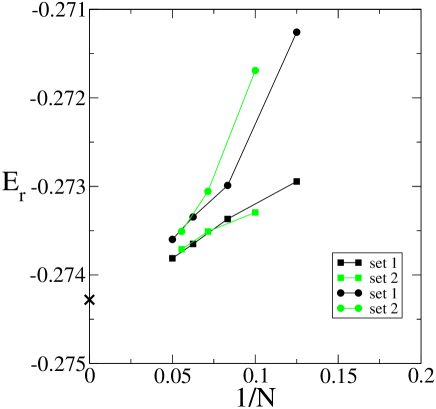
Figure 5: Resonance Energy for the two bundles (dots and squares) showed in Figure 3. Since there is an even-odd behavior the points of each bundle are grouped in two sets. Data in sets 1 ( Black ) correspond to $N=8,12,16,20$, and for sets 2 (green) correspond to $N=10,14,18$. The black cross shows the width calculated using complex scaling.

V Scaling of the resonance width

Many real algebra methods to calculate resonance energies use a Golden Rule-like formula to calculate the resonance width. In this section we will use the formula and stabilization procedure proposed by Tucker and Truhlar tucker1987 that we will describe briefly for completeness. This projection formula seems to work better for one-particle models. For two-particle models its utility has been questioned manby1997 , so to analyze the width of the resonance states of the quantum dot model we fitted the corresponding DOS using Equation (10).

The method of Tucker and Truhlar tucker1987 is implemented by the following steps. Choose a basis $\left\{\phi_{j}(\eta)\right\}$ where $\eta$ is a non-linear parameter. Diagonalize the Hamiltonian using up to $N$ functions of the basis. Look for the stabilization value ${\mathcal{E}}_{res}$ and its corresponding eigenfunction $\psi_{res}$ which are founded for some value $\eta^{r}$. Define the projector

$$Q^{\eta}=\left|\psi^{r,\eta}\right\rangle\left\langle\psi^{r,\eta}\right|,$$ (11)

where $\left|\psi^{r,\eta}\right\rangle$ is the normalized projection of $\psi_{res}$ onto the basis $\left\{\phi_{j}(\eta)\right\}_{j=1}^{N}$ for any other $\eta$.

Diagonalize the Hamiltonian $\tilde{H}=(1-Q^{\eta})H(1-Q^{\eta})$ in the basis $\left\{\phi_{j}(\eta)\right\}_{j=1}^{N}$, again as a function of $\eta$, and find a value $\eta^{c}$ of $\eta$ such that

$$E_{n}(\eta^{c})={\mathcal{E}}_{res},$$ (12)

where $E_{n}(\eta^{c})$ denotes eigenvalue $n$ of the projected Hamiltonian for the scale factor $\eta^{c}$, and $\chi_{n}(\eta^{c})$ is the corresponding eigenfunction.

With the previous definitions and quantities, the resonance width $\Gamma$ is given by

$$\Gamma=2\pi\rho(\eta^{c},{\mathcal{E}}_{res})\left|\right\langle\psi_{res}\left|H\right|\chi_{n}(\eta^{c})\left\rangle\right|^{2},$$ (13)

where

$$\rho(\eta^{c},{\mathcal{E}}_{res})=2/\left[E_{n+1}(\eta^{c})-E_{n-1}(\eta^{c})\right].$$ (14)

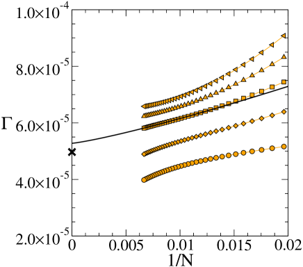
Figure 6: Scaling of the width vs. the inverse basis-set size $N$. All points correspond to the same bundle of states $(N=51,54,57,\ldots,150\,;\,m=17,18,19,\ldots,50)$. The curves were obtained with different values of the projection eigenvalue $n$ ( $1,2,3,4,5$, from bottom to top) . The black line is a fit for $n=3$ (Equation (17)) and the lowest $n$ curve that shows a scaling exponent greater than one ($\gamma(3)\sim 1.2$).

Despite some useful insights, the procedure sketched above does not determine all the intervening quantities, for instance there are many solutions to equation (12) and, of course, the stabilization method provides several good candidates for $\psi_{res}$ and $\eta^{r}$.

We are able to avoid some of the indeterminacies associated to the Tucker and Truhlar procedure using a bundle of states associated to a crossing, so $\psi_{res}$ and $\eta^{r}$ are given by any of the eigenfunctions associated to a bundle and $\eta^{r}(N,m)$ comes from the stabilization procedure. Then we construct projectors

$$Q^{\eta}_{N,m}=\left|\psi_{N}^{m}(\eta)\right\rangle\left\langle\psi_{N}^{m}(\eta)\right|,$$ (15)

where $\psi_{N}^{m}(\eta)$ is one of the variational eigenstates that belong to a bundle of states. With the projectors $Q^{\eta}_{N,m}$ we construct Hamiltonians $\tilde{H}$, and find the solutions to the problem

$$E_{n}(\eta_{n}^{c})={\mathcal{E}}_{res}.$$ (16)

Since there is not an a priori criteria to choose one particular solution of Equation (16) we show our numerical findings for several values of $n$. Figure 6 shows the behaviour of the resonance width calculated with Equation (13), where we have used $\psi_{51}^{17},\,\psi_{54}^{18},\,\psi_{57}^{19},\ldots$ as $\psi_{res}$ and $\chi_{n}$, where $n=1,2,3,4$ and $5$.

Despite that the different sets corresponding to different values of $n$ do not converge to any definite value, for $N$ large enough all the sets scale as $N^{-\gamma(n)}$, with $\gamma(n)>0$. Since the resonance energy scales as $N^{-1}$, at least when a bundle of states with a crossing is chosen to calculate approximations (see Figure 4), we suggest that the right scaling for $\Gamma$ is given by $\gamma=1$. Of course for a given basis size, particular variational functions, stabilization procedures and so on, we can hardly expect to find a proper set of $\Gamma$ whose scaling law would be $N^{-1}$. Instead of this we propose that the data in the right panel can be fitted by

$$\Gamma_{N,n}\sim A(\gamma(n))+B(\gamma(n))N^{-\gamma(n)},\quad\gamma(n)>0.$$ (17)

Then the best approximation for the resonance width is obtained fitting the curve and selecting the $\Gamma_{b}$ as $A(\gamma(n))$ for $\gamma(n)$ the closest value to one.

Figure 7: (color on-line) Resonance widths for the two bundles (dots and squares) showed in Figure 3. Since there is an even-odd behavior the points of each bundle are grouped in two sets. As in figure 5, data in sets 1 ( Black ) correspond to $N=8,12,16,20$, and for sets 2 (green) correspond to $N=10,14,18$. The widths where calculated using the method described in Reference kar2004 . The black cross is the width calculated using complex scaling.

As pointed in Reference manby1997 , the projection technique to calculate the width of a resonance can be implemented if a suitable form of the projection operator can be found. As this procedure is marred by several issues we used the DOS method to obtain the approximate widths of a resonance state of the two particle model. Figure 7 shows the widths calculated associated to the energies shown in Figure 5, the parameters of the Hamiltonian are exactly the same.

There is no obvious scaling function that allows the extrapolation of the data but, even for moderate values of $N$, it seems as the data converge to the value obtained using complex scaling.

VI Conclusions

In this work we analyzed the convergence properties of real ${\cal L}^{2}$ basis-set methods to obtain resonance energies and lifetimes. The convergence of the energy with the basis-set size for bound states is well understood, the larger the basis set the better the results and these methods converge to the exact values for the basis-set size going to infinite (complete basis set). This idea is frequently applied to resonance states. The increase of the basis-set size in some commonly used methods does not improve the accuracy of the value obtained for the resonance energy $E_{r}$, as showed in Figure 1. This undesirable behavior comes from the fact that the procedure is not variational as in the case of bound states. Moreover, the exact resonance eigenfunction does not belong to the Hilbert space expanded by the complete basis set. In this work we presented a prescription to pick a set or bundle of states that has linear convergence properties for small width resonances. This procedure is robust because the choice of different bundles results in very similar convergence curves and energy values. In fact, in the method described here, the pairs $(N,m)$ of the bundles play the role of a second stabilization parameter together with the variational parameter $\eta$. of a second We tested the method in others one and two particle systems and the general behavior of them is the same. The results are very good in all cases leading to an improvement in the calculation of the resonance energies. Nevertheless we have to note that the method could no be applied in cases where two or more resonance energies lie very close because the overlapping bundles.

The lifetime calculation is more subtle. The use of golden-rule-like formulas, as we applied here, always give several possible outcomes for the width $\Gamma_{N,n}$, corresponding to different pseudo-continuum states $\left|\chi_{n}\right\rangle$. The projection technique, Equation (13), is not the exception and it is not possible to select a priori which value of $\left\{\Gamma_{N,n}\right\}$ is the most accurate. The linear convergence of the DOS with basis-set size suggests that the scaling in the lifetime value, in accordance with the Energy scaling, should be linear. Regrettably, the projection method gives discrete sets of values which cannot be tuned to obtain an exact linear convergence. Our recipe is to choose the set $\Gamma_{N,n}$ whose scaling is closest to the linear one, then the best estimation for the resonance width is obtained from extrapolation.

Many open questions remain on the analysis of the different convergence properties of resonance energy and lifetime. The method presented here to obtain the resonance energy from convergence properties works very well, but the appearance of bundles in the spectrum is not completely understood. Even there is not a rigorous proof, the numerical evidence supports the idea that the behaviour of the systems studied here is quite general.

*

Appendix

In this appendix we give arguments that support our assumptions on the scaling of the eigenenergies with the basis-set parameter $\eta$. We present our argument for one body Hamiltonians, but it is straightforward to generalize to more particles with pair interactions decaying fast enough at large distances.

First et all, we present two very known results that we need later.

1. Let $A$ be an $n\times n$ matrix with all its matrix elements having the form $a_{i,j}(\eta)=a_{i,j}(1)\,f(\eta)$, where $f(1)=1$, then if $f(\eta)\neq 0$ the eigenvalues of $A$ scales with $f(\eta)$:

   $$det[A(\eta)-\lambda(\eta)\,I]=0\;\Rightarrow det[A(1)-\frac{\lambda(\eta)}{f(\eta)}\,I]=0\Rightarrow\lambda(1)=\frac{\lambda(\eta)}{f(\eta)}\,.$$ (18)

2. Let $A,\,B$ $n\times n$ be symmetric matrices with $|b_{i,j}|<const.$, and $\alpha_{i},\,\beta_{i},\,\lambda_{i},\;i=1,\cdots,n$ the eigenvalues of $A,\,B$ and $A+\varepsilon B$ respectively, in nondecreasing order, then, by the minimax principle wilkinson65

$$\alpha_{i}+\varepsilon\beta_{1}\leq\lambda_{i}\leq\alpha_{i}+\varepsilon\beta_{n}$$ (19)

Consider a spherical one-particle potential with compact support, $v(r)=0$ if $r>R$, and finite, $|v(r)|<\infty\;\forall r$ (both conditions could be relaxed, but we adopt them for simplicity). Let the basis-set functions be of the form $\Phi_{n}(\eta,r)=c_{n}(\eta)\,\Phi_{n}(\eta r)$ with $||\Phi_{n}(\eta,r)||=1$ and $c_{n}(1)=1$, then the coefficients take the form $c_{n}(\eta)=c_{n}(1)\eta^{3/2}$.

With these assumptions, the matrix elements for the kinetic energy are

$$\begin{array}[]{l}T_{m,n}(\eta)\,=\,c^{*}_{m}(1)c_{n}(1)\,\eta^{3}\,\int\;d^{3}x\Phi_{m}(\eta,r)\frac{1}{r^{2}}\,\frac{\partial}{\partial r}\,\left(r^{2}\frac{\partial}{\partial r}\right)\Phi_{n}(\eta,r)\,=\\ \mbox{}\\ c^{*}_{m}(1)c_{n}(1)\,\eta^{2}\,\int\;d^{3}x\;\Phi_{m}(1,r)\frac{1}{r^{2}}\,\frac{\partial}{\partial r}\,\left(r^{2}\frac{\partial}{\partial r}\right)\Phi_{n}(1,r)\,=\,\eta^{2}T_{m,n}(1)\,,\end{array}$$ (20)

and then, by Equation (18), all the eigenvalues of the kinetic energy have the same scaling with $\eta^{2}$. We have to show that, in both limits, $\eta\rightarrow 0$ and $\eta\rightarrow\infty$, for all the potential matrix elements hold $v_{m,n}/\eta^{2}\ll 1$, and then, by the Wielandt-Hoffman theorem wilkinson65 , the eigenenergies are a perturbation of the eigenvalues of the kinetic energy.

$\eta\rightarrow 0$

In this limit $\eta\,R\ll 1$ $\Phi(\eta r)\simeq\Phi(0)$ for $r\varepsilon(0,R]$, then

$$v_{m,n}\simeq\left[4\,\pi\,\Phi^{*}_{m}(1,0)\,\Phi(1,0)\,\int_{0}^{R}\,r^{2}\,dr\,v(r)\right]\;\eta^{3}\,=\,\hat{v}_{m,n}\,\eta^{3}\,,$$ (21)

where $\hat{v}_{m,n}$ do not depend on $\eta$. Then, in this limit $v_{m,n}/\eta^{2}\sim\eta\ll 1$.

$\eta\rightarrow\infty$

For $\eta\,R\rightarrow\infty$ we obtain for the potential matrix elements

$$\begin{array}[]{ll}v_{m,n}\,=&c^{*}_{m}(1)c_{n}(1)\,\eta^{3}\,\int_{0}^{R}\,r^{2}\,dr\,\Phi^{*}_{m}(\eta\,r)\,v(r)\,\Phi(\eta\,r)\,=\\ \mbox{}&\mbox{}\\ \mbox{}&c^{*}_{m}(1)c_{n}(1)\,\int_{0}^{\eta R}\,r^{2}\,dr\,\Phi^{*}_{m}(r)\,v(r/\eta)\,\Phi(r)\,\simeq\\ \mbox{}&\mbox{}\\ \mbox{}&c^{*}_{m}(1)c_{n}(1)\,v(0)\,\int_{0}^{\eta R}\,r^{2}\,dr\,\Phi^{*}_{m}(r)\,\Phi(r)\,\stackrel{{\scriptstyle\longrightarrow}}{{\eta\rightarrow\infty}}\\ \mbox{}&\mbox{}\\ \mbox{}&c^{*}_{m}(1)c_{n}(1)\,v(0)\,.\end{array}$$ (22)

Then also in this limit we obtain $v_{m,n}/\eta^{2}\sim 1/\eta^{2}\ll 1$.

- (1) N Moiseyev, Phys. Rep. 302, 211 (1998).
- (2) W P Reinhardt and S Han, Int. J. Quant. Chem. 57, 327 (1996).
- (3) Y Sajeev and N Moiseyev, Phys. Rev. B 78, 075316 (2008).
- (4) M Bylicki, W Jaskólski, A Stachów and J Diaz, Phys. Rev. B 72, 075434 (2005).
- (5) J Dubau and I A Ivanov, J. Phys. B: At. Mol. Opt. Phys. 31 3335 (1998).
- (6) A T Kruppa and K Arai, Phys. Rev. A 59, 3556 (1999).
- (7) S Kar and Y K Ho, J. Phys. B: At. Mol. Opt. Phys. 37, 3177 (2004).
- (8) B Simon, Int. J. Quant. Chem. 14, 529 (1978).
- (9) N Moiseyev, S Friedland, Phys. Rev. A 22, 618 (1980).
- (10) N Moiseyev, S Friedland, P R Certain, J. Chem. Phys. 78, 4739 (1981).
- (11) Y Sajeev, V Vysotskiy, L S Cederbaum, and N Moiseyev, J. Chem. Phys. 131, 211102 (2009).
- (12) F M Pont, O Osenda, P Serra and J H Toloza, Phys. Rev. A 81, 042518 (2010).
- (13) F M Pont, O Osenda and P Serra, Phys. Scr. 82, 038104 (2010).
- (14) S Kar and Y K Ho, Phys. Rev. 75, 062509 (2007).
- (15) S Kar and Y K Ho, Phys. Rev. 76, 032711 (2007).
- (16) E Holien and J Midtdal, J. Chem. Phys. 45, 2209 (1966).
- (17) V A Mandelshtam, T R Ravuri and H S Taylor, Phys. Rev. Lett. 70, 1932 (1993).
- (18) S Kais and P Serra, Adv. Chem. Phys. 125, 1 (2003).
- (19) A V Sergeev and S Kais, Int. J. Quant. Chem. 82, 255 (2001).
- (20) K M Sluis and E. A. Gislason, Chem. Phys. Lett. 165, 195 (1990).
- (21) B J Hellmann, J. Chem. Phys. 3, 61 (1935).
- (22) A V Sergeev and S Kais, Int. J. Quant. Chem. 75, 533 (1999).
- (23) A L Frapiccini, J M Randazzo, G Gasaneo, F D Colavecchia, Int. J. Quant. Chem. 110, 963 (2009).
- (24) C H Maier, L S Cederbaum and W. Domcke, J. Phys. B: Atom. Molec. Phys. 13, L119 (1980).
- (25) A U Hazi and H S Taylor, Phys. Rev. A 14, 2071 (1976).
- (26) A Ferrón, O Osenda and P Serra, Phys. Rev. A 79, 032509 (2009).
- (27) H Feschbach, Ann. Phys. NY 19, 627 (1962)
- (28) N Moiseyev, C Corcoran, Phys. Rev. A 20, 814 (1979).
- (29) M E Fisher, In Critical Phenomena, Proceedings of the 51st Enrico Fermi Summer School, Varenna, Italy, M. S. Green, ed. (Academic Press, New York 1971).
- (30) S E Tucker and D. G. Truhlar, J.Chem. Phys. 86, 6251 (1987).
- (31) F R Manby and G Doggetty, J. Phys. B: At. Mol. Opt. Phys. 30, 3343 (1997)
- (32) J. H. Wilkinson, The Algebraic Eigenvalue Problem, Oxford University Press, London, (1965).