Lorentz-covariant perturbation theory for relativistic gravitational bremsstrahlung

Abstract

We formulate Lorentz-covariant classical perturbation theory to deal with relativistic bremsstrahlung under gravitational scattering. Our approach is a version of the fast motion approximation scheme, the main novelty being the use of the momentum space representation. Using it we calculate in a closed form the spectrum of scalar, electromagnetic and gravitational radiation. Our results for the total emitted energy agree with those by Thorne and Kovacs. We also explain why the method of equivalent gravitons fails to produce the correct result for the spectral-angular distribution of emitted radiation under gravitational scattering, contrary to the case of Weizsäcker-Williams approximation in quantum electrodynamics.

I Introduction

Gravitational radiation by non-relativistic and quasi-relativistic systems is low-multipole and can be easily calculated using the quadrupole formula of General Relativity with higher multipole corrections. With increasing velocities, the contribution from higher multipoles becomes dominant, so one needs another technique. The most adequate approach is the method of post-linear expansions which was discussed in early 60-ies most notably by Bertotti B , Bertotti and Plebanski BP , Havas and Goldberg HG ; Goldberg (see also H ; R ; K ; SH ; In ; An ; Ros ; CS ; WeGo ). We have developed a momentum space version of this approach GG1 which is applied here to gravitational bremsstrahlung. Although technically different, our calculations essentially overlap and agree with those by Thorne and collaborators CT ; KT3 ; KT4 . The results also agree with an alternative calculations by Peters Pe1 ; Pe2 ; Pe3 based on the linear perturbation theory on Schwarzschild background. They disagree, however, with calculations based on “equivalent gravitons” method MaNu , and we explain the origin of this disagreement.

Other approaches to relativistic bremsstrahlung problem are worth to be mentioned. One, suggested by D’Eath DE , is based on replacing the boosted Schwarzschild metric by the impulsive gravitational wave. Another, due to Smarr Sm1 ; Sm2 , appeals to calculation of the radiation amplitude in the low-frequency region. This overlaps with quantum calculation of the cross-section in the Born approximation Barker .

To calculate the leading order gravitational radiation in relativistic collisions of particles interacting predominantly through the non-gravitational forces it is enough to use the linearized gravity on Minkowski background. In the case of gravitational interaction we need at least the next post-linear order. If one interprets the second order gravitational potentials in terms of Minkowski space coordinates, one finds that the source of gravitational radiation becomes non-local due to contribution of the first order gravitational stresses (similarly for non-gravitational radiation from particles interacting by gravity). This non-locality leads to destructive interference of high frequency part of radiation, so the spectrum will be different from that of the electromagnetic bremsstrahlung.

II Field equations in quasilinear form

Consider a system of point particles, interacting by non-gravitational fields (scalar $\psi$ or massless vector $A^{\mu}$) and moving in a self-consistent gravitational field described by the metric $g_{\mu\nu}$. The action can be presented as $S=S_{p}+S_{\psi}+S_{A}+S_{g},$ where $S_{p}$ is the sum of particle actions including non-gravitational interaction terms

$$S_{p}=-\sum\int(m+f\psi+eA_{\mu}{\dot{x}}^{\mu})ds,$$ (1)

$S_{\psi}$and $S_{A}$ are scalar and Maxwell field actions

$$S_{\psi}=\frac{1}{8\pi}\int\partial_{\mu}\psi\,\partial^{\mu}\psi\sqrt{-g}d^{4}x,\quad S_{A}=-\frac{1}{16\pi}\int F_{\mu\nu}F^{\mu\nu}\sqrt{-g}d^{4}x,$$ (2)

and the gravitational lagrangian is taken in the two-gamma form:

$$S_{g}=\int{\cal L}\sqrt{-g}d^{4}x,\quad{\cal L}=-\frac{1}{2\kappa^{2}}\int g^{\mu\nu}\left(\Gamma_{\mu\beta}^{\alpha}\Gamma_{\nu\alpha}^{\beta}-\Gamma_{{\mu\nu}}^{\alpha}\Gamma_{\alpha\beta}^{\beta}\right),\quad\kappa^{2}=8\pi G.$$ (3)

Assuming gravitational field to be negligible at spatial infinity, we choose asymptotically Minkowskian metric $\eta_{\mu\nu}$ in this region and introduce the (non-tensor) metric deviation variable

$$h_{{\mu\nu}}=g_{{\mu\nu}}-\eta_{{\mu\nu}}\ .$$ (4)

Then for $r\rightarrow\infty$ one has $h_{{\mu\nu}}\rightarrow 0$, but $h_{{\mu\nu}}$ are not necessarily small everywhere. By convention, the indices of the quantities $h_{{\mu\nu}},\ \partial_{\mu}$ and $\eta_{{\mu\nu}}$ will be raised and lowered by the Minkowski metric $\eta_{{\mu\nu}}$ , while the indices of the true tensors are operated with the metric $g_{{\mu\nu}}$.

Introducing an antisymmetric tensor density

$$H^{\alpha\nu\beta\lambda}=g\left(g^{\alpha\lambda}g^{\beta\nu}-g^{\alpha\beta}g^{\lambda\nu}\right),$$ (5)

one can present Einstein equations in a divergence form

$$\left(H^{\alpha\nu\beta\lambda}_{,\beta}\;g_{\lambda\mu}\;/\sqrt{-g}\right)_{,\alpha}=-2\kappa^{2}\sqrt{-g}\left(T^{\nu}_{\mu}+t^{\;\,\nu}_{\mu}\right),$$ (6)

where $T^{\nu}_{\mu}$ is the total matter stress-tensor, and $t^{\;\,\nu}_{\mu}$ is Einstein’s canonical pseudotensor

$$t^{\;\,\nu}_{\mu}\;=\;\frac{1}{\sqrt{-g}}\;g^{\alpha\beta}_{\mu}\;\frac{\partial(\sqrt{-g}\;{\cal L})}{\partial g^{\alpha\beta}_{\nu}}-\delta^{\nu}_{\mu}{\cal L}.$$ (7)

Maxwell equations can be written in a similar form

$$\left(H^{\alpha\nu\beta\lambda}_{,\beta}\;g_{\lambda\mu}\;/\sqrt{-g}\right)_{,\alpha}=-4\pi\;\sqrt{-g}\;j^{\mu},$$ (8)

where the vector-current is

$$j^{\mu}=\sum e\int ds\;{\dot{x}}^{\mu}\;\delta^{4}(x-x(s))/\sqrt{-g}.$$ (9)

Finally, the scalar wave equation reads

$$\left(\psi_{,\mu}\;g^{\mu\nu}\;\sqrt{-g}\right)_{,\nu}=4\pi\;\sqrt{-g}\;\tau,$$ (10)

with the scalar current

$$\tau=\sum f\int ds\;\delta^{4}(x-x(s))/\sqrt{-g}.$$ (11)

Particle equations of motion generically read

$$\frac{d}{ds}\left[(m-f\psi)\right]{\dot{x}}_{\mu}=\frac{m}{2}g_{\alpha\beta,\mu}{\dot{x}}^{\alpha}{\dot{x}}^{\beta}\;-mf\psi_{,\mu}\;+\;eF_{\mu\nu}\;{\dot{x}}^{\nu}.$$ (12)

All the above equations are exact and can be regarded as a system defining the particle motion and evolution of the scalar, vector and gravity fields and in a self-consistent way. However, since the notion of delta-functions is not defined in the full non-linear general relativity, we can deal with point particles only perturbatively, expanding all the quantities in formal series in the gravitational coupling $\kappa$. For this one has to pass first to quasilinear form of the field equations. For Einstein equations we single out the linear part of the $H$-tensor:

$$H^{\alpha\nu\beta\lambda}=\eta^{\alpha\beta}\eta^{\lambda\nu}-\eta^{\alpha\lambda}\eta^{\beta\nu}+{\cal L}^{\alpha\nu\beta\lambda}+{\cal N}^{\alpha\nu\beta\lambda}$$ (13)

where ${\cal L}^{\alpha\nu\beta\lambda}$ joins terms linear in $h_{\mu\nu}$:

$${\cal L}^{\alpha\nu\beta\lambda}=\psi^{\alpha\lambda}\eta^{\beta\nu}+\psi^{\beta\nu}\eta^{\alpha\lambda}-\psi^{\alpha\beta}\eta^{\lambda\nu}-\psi^{\lambda\nu}\eta^{\alpha\beta},\quad\psi^{\mu\nu}=h^{\mu\nu}-\frac{1}{2}\eta^{\mu\nu}\psi_{\lambda}^{\lambda},$$ (14)

while ${\cal N}^{\alpha\nu\beta\lambda}$ denotes non-linear in $h_{\mu\nu}$ terms. Gravitational equations can be now presented as

$${\cal L}^{\lambda\alpha\beta\tau}_{,\alpha\beta}\eta_{\mu\lambda}\eta_{\nu\tau}=2\kappa^{2}\tau_{\mu\nu},\quad\tau_{\mu\nu}=T_{\mu\nu}+S_{\mu\nu},$$ (15)

where in $S_{\mu\nu}$ all the non-linear terms are collected. To calculate gravitational radiation one needs only terms quadratic in $h_{\mu\nu}$.

Maxwell equations can be rewritten similarly:

$$A_{\alpha,\beta\nu}(\eta^{\alpha\mu}\eta^{\beta\nu}-\eta^{\alpha\nu}\eta^{\beta\mu})=4\pi(j^{\mu}+S^{\mu})\;\sqrt{-g},$$ (16)

where an effective “gravitational” vector current is given by

$$\sqrt{-g}S^{\mu}=\left[\left(1/\sqrt{-g}-1\right)(\eta^{\alpha\mu}\eta^{\beta\nu}-\eta^{\alpha\nu}\eta^{\beta\mu})+\left({\cal L}^{{\mu\nu}\alpha\beta}+{\cal N}^{{\mu\nu}\alpha\beta}\right)A_{\beta,\alpha}\right]_{,\nu}.$$ (17)

In the scalar case we obtain similarly:

$$\psi_{,\mu}^{,\mu}=-4\pi f(\tau+S)\ ,$$ (18)

where

$$S=(1/{4\pi f})\sigma_{,\mu}^{\mu}\ ,\quad\sigma^{\mu}=(\sqrt{-g}g^{{\mu\nu}}-\eta^{{\mu\nu}})\psi_{,\nu}\ .$$

This looks as the flat space wave equation for the spin zero field, with an important difference, however, that the “source” depends explicitly on $\psi$.

Now we can further simplify the quasilinear equations (which are still exact in all orders in $\kappa$) imposing the gauge conditions

$$\psi_{{\mu\nu},\lambda}\eta^{\nu\lambda}=0,\qquad A_{\mu,\nu}\eta^{\mu\nu}=0,$$ (19)

which are consistent with the field equations by virtue of the identities:

$$\tau_{{\mu\nu},\lambda}\eta^{\nu\lambda}=0,\qquad\left(\sqrt{-g}\;S^{\mu}\right)_{,\mu}=\left(\sqrt{-g}\;j^{\mu}\right)_{,\mu}.$$ (20)

In this gauge Einstein and Maxwell equations read

$$\Box\psi_{\mu\nu}=2\kappa^{2}\tau_{\mu\nu},\quad\Box A_{\mu}=-4\pi\sqrt{-g}(j^{\lambda}+S^{\lambda})\eta_{\lambda\mu},$$ (21)

with $\Box=-\partial_{\lambda}\partial_{\tau}\eta^{\lambda\tau}$.

III Scalar bremsstrahlung under gravitational scattering

Consider two point masses $m_{1}$ and $m_{2}$, one of which ($m_{1}$) carries the scalar charge $f$. Particles interact via gravity and the systems emits both gravitational and scalar waves. In this section we calculate scalar radiation. The action reads

$$S=-\int(m_{1}+f\psi(x))\sqrt{\dot{x_{1}}^{2}}ds-m_{2}\int\sqrt{\dot{x_{2}}^{2}}ds+\frac{1}{8\pi}\int\sqrt{-g}d^{D}x\partial_{\mu}\psi\,\partial^{\mu}\psi\,$$ (22)

where $\dot{x}^{2}\equiv g_{\alpha\beta}\dot{x}^{\alpha}\dot{x}^{\beta}$, dot denotes differentiation with respect to the interval $s$, and the metric signature is mostly minus.

The full system of equations describing the collision consists of Einstein equations, scalar field equation and particle equations as given in the previous section. The total loss of the four-momentum during the collision can be presented as

$$\Delta P_{S}^{\mu}=\int_{-\infty}^{\infty}dt\oint T_{\psi}^{\mu i}d\sigma_{i}\ ,$$ (23)

where

$$T_{\psi}^{{\mu\nu}}=\frac{1}{4\pi}\left(\psi_{,\mu}\psi_{,\nu}-\frac{1}{2}\psi_{,\alpha}\psi^{,\alpha}\right)$$ (24)

is the energy-momentum tensor of the massless field $\psi$, and integration is performed over the sphere of infinite radius. The non-zero contribution comes from the terms in $T_{\psi}^{\mu i}$, which fall off at infinity as $r^{-2}$. Also, without changing the integral, one can add to the integrand the total derivative over time $(\psi^{,\mu}\psi^{,0}-(1/2)\eta^{\mu 0}\psi_{,\alpha}\psi^{,\alpha})_{,0}$. Then, applying the Gauss theorem we can transform the Eq. (23) to the following form:

$$\Delta P_{S}^{\mu}=\frac{1}{4\pi}\int d^{4}x\ \psi^{,\mu}\psi_{,\nu}^{,\nu}\ .$$ (25)

To exclude an infinite self-energy part it is enough to substitute as $\psi_{,\nu}^{,\nu}$ the right hand side of the Eq. (18), while as $\psi$ – the $t$-odd part of the retarded potential

$$\psi(x)=-\frac{if}{(2\pi)^{2}}\int d^{4}ke^{-ikx}\varepsilon(k^{0})\delta(k^{2})[\tau(k)+S(k)]\ ,$$ (26)

where $\varepsilon(k^{0})=\theta(k^{0})-\theta(-k^{0})$ is the sign function and the Fourier transforms are defined as

$$\tau(k)=\int d^{4}xe^{ikx}\tau(x)\$$ (27)

and similarly for $S(k)$. We obtain:

$$\Delta P_{S}^{\mu}=\frac{f^{2}}{2\pi^{2}}\int d^{4}kk^{\mu}\theta(k^{0})\delta(k^{2})\mid\tau(k)+S(k)\mid^{2}\ .$$ (28)

This expression is analogous to the usual one in electrodynamics, differing from it by presence of the non-local current $S(k)$ which we will call the stress current.

To find $\tau(k)$ and $S(k)$ we will solve the Einstein equation, the particle equations and the scalar field equation (18) expanding $g_{{\mu\nu}},\ \psi$ and $x^{\mu}$ in powers of the gravitational constant $G$. The actual expansion parameter in the ultrarelativistic collision problem will be the ratio of the gravitational radius of one of the particle to the impact parameter. One can show that approximation is valid if the particle scattering angle is small with respect to the radiation angle We

$$G(m_{1}+m_{2})/{\rho v^{2}}\ll 1/{\gamma}\ ,$$ (29)

where $\gamma=(1-v^{2})^{-1/2},\ v$ – the relative velocity of the colliding particles, $\rho$ – the impact parameter.

We parameterize the particles world lines as

$$x_{1}^{\mu}=\Delta^{\mu}+(p_{1}^{\mu}/m_{1})s_{1}+\tilde{x}_{1}^{\mu}(s_{1})\ ,$$

$$x_{2}^{\mu}=(p_{2}^{\mu}/m_{2})s_{2}+\tilde{x}_{2}^{\mu}(s_{2})\ ,$$ (30)

with $\sqrt{-\Delta^{2}}=\rho,(\Delta p_{1})=(\Delta p_{2})=0,\Delta^{\mu}$ – is the four-vector which in the rest frame of the second particle takes the form $(0,\vec{\rho})$. Here and below we use brackets $(\ldots)$ to denote scalar products with respect to Minkowski metric. We choose the initial conditions

$$\tilde{x}_{a}^{\mu}(-\infty)=d\tilde{x}_{a}^{\mu}/ds(-\infty)=0,\ a=1,2\ ,$$ (31)

so that $p_{a}^{\mu}$ is the four-momentum of the particle $a$ before the collision, and $\eta^{{\mu\nu}}p_{a}^{\mu}p_{a}^{\nu}=m_{a}^{2};\ \tilde{x}_{a}^{\mu}$ is the correction due to the gravitational interaction.

In the lowest order in gravitational interaction the correction to the space-time metric $\eta_{{\mu\nu}}$ due to the second particle reads

$$h_{2}^{{\mu\nu}}(x)=\frac{2G}{\pi^{2}}\left(p_{2}^{\mu}p_{2}^{\nu}-\frac{1}{2}m_{2}^{2}\eta^{{\mu\nu}}\right)\int d^{4}k\frac{\delta(kp_{2})}{k^{2}}e^{-ikx}\ .$$ (32)

Substituting this into the equation of motion of the particle $m_{1}$ we find

$$\tilde{x}_{1}^{\mu}(s)=-i\frac{G}{\pi^{2}}\int d^{4}q\frac{\delta(qp_{2})}{q^{2}(qp_{1})^{2}}e^{-iq(\Delta+\frac{p_{1}}{m_{1}}s)}\biggl{\{}2(qp_{1})\left[(p_{1}p_{2})p_{2}^{\mu}-\frac{m_{2}^{2}}{2}p_{1}^{\mu}\right]-\left[(p_{1}p_{2})^{2}-\frac{(m_{1}m_{2})^{2}}{2}\right]q^{\mu}\biggr{\}}\ .$$ (33)

To calculate the Fourier-transform of $S$ we use the expression for $\psi$ in the lowest order (zero order in $G$)

$$\psi(x)=\frac{fm_{1}^{2}}{2\pi^{2}}\int d^{4}k\frac{\delta(kp_{1})}{k^{2}}e^{-ik(x-\Delta)}\ .$$ (34)

The Fourier-transforms $\tau(k)$ and $S(k)$ can be computed as follows. Using the integrals

$$\int d^{4}qe^{-iq\Delta}\frac{\delta(qp_{2})\delta(qp_{1}-kp_{1})}{q^{2}}=-\frac{2\pi}{I}K_{0}(z_{1})\ ,$$

$$\int d^{4}qe^{-iq\Delta}q^{\mu}\frac{\delta(qp_{2})\delta(qp_{1}-kp_{1})}{q^{2}}=2\pi\frac{m_{2}^{2}(kp_{1})}{I^{3}}\biggl{\{}\biggl{[}p_{1}^{\mu}-\frac{(p_{1}p_{2})}{m_{2}^{2}}p_{2}^{\mu}\biggr{]}K_{0}(z_{1})-i(kp_{1})\Delta^{\mu}\frac{K_{1}(z_{1})}{z_{1}}\biggr{\}}\ ,$$ (35)

we obtain

$$\tau(k)=-4Gm_{1}m_{2}e^{ik\Delta} \biggl{\{}\biggl{[}\biggl{(}1-\frac{(m_{1}m_{2})^{2}}{2I^{2}}\biggr{)}\frac{(p_{1}p_{2})}{I}\frac{z_{2}}{z_{1}}+\frac{(m_{1}m_{2})^{3}}{2I^{3}}\biggr{]}K_{0}(z_{1})-$$

$$-i(k\Delta)\frac{m_{1}m_{2}}{I}\biggl{(}1+\frac{(m_{1}m_{2})^{2}}{2I^{2}}\biggr{)}\frac{K_{1}(z_{1})}{z_{1}}\biggr{\}}\ ,$$ (36)

where $I=\{(p_{1}p_{2})^{2}-(m_{1}m_{2})^{2}\}^{1/2}\ ,\quad z_{1}=\sqrt{-\Delta^{2}}(kp_{1})m_{2}I^{-1}\ ,\quad z_{2}=\sqrt{-\Delta^{2}}(kp_{2})m_{1}I^{-1}\,\quad K_{0,1}$ are the Macdonald functions. Lorentz-invariant integrals (III) an be conveniently computed in the rest frame of the second particle $p_{2}^{\mu}=(m_{2},0)$. Then two integrations from four are performed using the delta-functions, while the remaining two-dimensional integral in the plane orthogonal to ${\bf p_{1}}$ is computed using the polar coordinates. The angular integral is standard, and the last one is done by contour integration.

Integration over $d^{4}q$ in the expression for $S(k)$ can be done using the Feynman parameterization. We obtain

$$S(k)=4GIe^{ik\Delta}z_{2}^{2}\int_{0}^{1}dxe^{-ix(k\Delta)}\frac{K_{1}(z(x))}{z(x)}\ ,$$ (37)

where

$$z(x)=\sqrt{\xi^{2}(x)};\ \xi^{\mu}(x)=(1-x)z_{1}p_{2}^{\mu}/m_{2}+xz_{2}p_{1}^{\mu}/m_{1}\ ,$$

$$z(0)=z_{1}=\sqrt{-\Delta^{2}}(kp_{1})m_{2}/I;\ z(1)=z_{2}=\sqrt{-\Delta^{2}}(kp_{2})m_{1}/I\ .$$

The Eqs. (III) and (37) are obtained under the only restriction (29), they are valid for arbitrary velocities $v$. In the rest frame of the second particle $p_{2}^{\mu}=(m_{2},0)$ we further specify the coordinates so that

$$\vec{\rho}=(0,0,\rho)\ ,\qquad\vec{p}_{1}=(0,p_{1},0)\ ,$$

$$\vec{k}=\omega(\sin\theta\sin\phi,\cos\theta,\sin\theta\cos\phi)\ .$$

Consider the case of non-relativistic velocities. For $v\ll 1,\,z(x)=z_{1}=z_{2}=\omega\rho/v$, then the integral in (37) is easily done and we obtain

$$\tau(k)=\frac{2Gm_{1}m_{2}}{v^{2}}e^{-i\omega\rho\sin\theta\cos\phi}[\cos\theta K_{0}(a)-i\sin\theta\cos\phi K_{1}^{2}(a)]\ ,$$ (38)

$$S(k)=4Gm_{1}m_{2}vaK_{1}(a)e^{-i\omega\rho\sin\theta\cos\phi}\ ,$$ (39)

where $a=\omega\rho/v$. From (38) and (39) it is clear that $S/\tau\sim v^{3}$, so in the lowest in $v$ approximation radiation is entirely determined by the local current (38). Substituting it into the Eq. (28), after some simple transformations we find

$$\frac{d^{2}E_{S}}{d\omega d\Omega}=(\frac{Gfm_{1}m_{2}}{\pi\rho v})^{2}a^{2}[\cos^{2}\theta K_{0}^{2}(a)+\sin^{2}\theta\cos^{2}\phi K_{1}^{2}(a)]\ .$$ (40)

One can see that for small velocities the characteristic radiation frequency $\omega\sim v/\rho$ is inverse to the effective time of collision $\rho/v$.

The total energy loss during the collision can be obtained integrating (40) over angles and the frequency:

$$\Delta E_{S}=(\pi/6)(fGm_{1}m_{2})^{2}/\rho^{3}v\ .$$ (41)

In the ultrarelativistic case $(\gamma\gg 1)$ the effective spread of the stress current $S(x)$ is of the order of $\rho$. So it can be expected that for the wavelengthes $\lambda\gg\rho$ the source with act as point-like. Indeed, for $\omega\ll\rho^{-1}\ (\lambda\gg\rho)$ the argument of the Macdonald functions (III) and (37) is small for all values of parameters, and with account for the leading terms we obtain

$$\tau(k)=-i\frac{4Gm_{1}m_{2}}{\gamma}\frac{\sin\theta\cos\phi}{\omega\rho\delta^{2}},\ \frac{S(k)}{\tau(k)}\sim\omega\rho\ll 1\ ,$$ (42)

where $\delta=1-v\cos\theta$. Substituting (42) into (28) we find:

$$\frac{dE_{S}}{d\omega}=\frac{16}{3\pi}\frac{(fGm_{1}m_{2})^{2}}{\rho^{2}}\gamma^{2},\ \omega\ll\rho^{-1}\ .$$ (43)

In the frequency region $\omega\geqslant\rho^{-1}$ the contributions of the local and the non-local currents are of the same order. In this case for the spectral distribution of the total emitted energy we obtain:

$$\frac{dE_{S}}{d\omega}=\frac{16(fGm_{1}m_{2})^{2}}{\pi}\omega^{2}\int_{0}^{\infty}\int_{0}^{\infty}d\xi d\eta\frac{e^{-\frac{2\omega\rho}{\gamma}\sqrt{1+\xi^{2}}\sqrt{1+\eta^{2}}}}{(1+\xi^{2})^{3/2}(1+\eta^{2})^{1/2}}\ln\frac{1+\xi^{2}+\eta^{2}}{\eta^{2}}\ .$$ (44)

For $\rho^{-1}\leq\omega\ll\gamma/\rho$

$$\frac{dE_{S}}{d\omega}=\lambda_{S}\frac{(fGm_{1}m_{2})^{2}}{\rho^{2}}\gamma^{2}\biggl{(}\frac{\omega\rho}{\gamma}\biggr{)}^{2}\ ,$$ (45)

where

$$\lambda_{S}=\frac{64}{3\pi}\int_{0}^{\infty}dxx^{-3}\ln^{3}(x+\sqrt{1+x^{2}})\approx 8.$$

For relatively high frequencies $\omega\gg\gamma/\rho$ the integral in (44) is formed at $\xi,\ \eta\ll 1$. So approximately

$$\frac{dE_{S}}{d\omega}\simeq\frac{4(fGm_{1}m_{2})^{2}}{\rho^{2}}\gamma^{2}\biggl{(}\frac{\omega\rho}{\gamma}\biggr{)}\ln\frac{4e^{C}\omega\rho}{\gamma}e^{-\frac{2\omega\rho}{\gamma}}\ .$$ (46)

The expressions (43), (45) and (46) together describe the behavior of the spectral curve. It follows, in particular, that in the spectral distribution there is a maximum around the frequency $\omega\sim\gamma/\rho$. The total energy loss during the collision is obtained integrating (44) over the frequency:

$$\Delta E_{S}=\Lambda_{S}\frac{(fGm_{1}m_{2})^{2}}{\rho^{3}}\gamma^{3},\ \Lambda_{S}=\frac{3\tilde{G}}{2}+\frac{77}{12}-2\pi\simeq 1.51\ ,$$ (47)

where $\tilde{G}$ is the Catalan constant.

Let us compare these results with the case of the electromagnetic interaction in Minkowski space, when the source term in the equation for $\psi$ does not contain the stress current $S(x)$. Suppose that the colliding particles are electrically charged $(e_{1},e_{2})$ and neglect gravitational interaction with respect to electromagnetic one. Then as the source $\tau(k)$ in (28) one has to use the Fourier-transform of the trace of the particles energy-momentum tensor. After similar calculations we obtain:

$$T(k)=\frac{2e_{1}e_{2}(m_{1}m_{2})^{2}}{I^{3}}e^{ik\Delta}\biggl{\{}\biggl{[}(p_{1}p_{2})-m_{1}^{2}\frac{(kp_{2})}{(kp_{1})}\biggr{]}K_{0}(z_{1})-i(k\Delta)(p_{1}p_{2})\frac{K_{1}(z_{1})}{z_{1}}\biggr{\}}\ .$$ (48)

In the ultrarelativistic case $(\gamma\gg 1)$ the spectral-angular distribution is dominated by the second term in (48). In the rest frame of the second particle we find in the leading order in $\gamma$:

$$\frac{dE_{S}}{d\omega}=\frac{8}{\pi}\frac{(fe_{1}e_{2})^{2}}{\rho^{2}}z\int_{z}^{\infty}dx\frac{z}{x}\biggl{(}1-\frac{z}{x}\biggr{)}K_{1}^{2}(x)\ ,$$ (49)

where $z=\omega\rho/2\gamma^{2}$. Using the asymptotic expansions for the Macdonald functions for small and large arguments, from (49) we find for $\omega\ll\gamma^{2}/\rho$:

$$\frac{dE_{S}}{d\omega}=\frac{4}{3\pi}\frac{(fe_{1}e_{2})^{2}}{\rho^{2}}\ ,$$ (50)

while for high frequencies $\omega\gg\gamma^{2}/\rho$

$$\frac{dE_{S}}{d\omega}=2\frac{(fe_{1}e_{2})^{2}}{\rho^{2}}\frac{\gamma^{2}}{\omega\rho}e^{-\frac{\omega\rho}{\gamma^{2}}}\ .$$ (51)

Note, that for the local source case our methods gives the energy loss without restrictions on the relative velocity of collision. Indeed, substituting (48) into (28) and integrating over frequencies and angles we obtain

$$\Delta E_{S}=\frac{\pi}{8}\frac{(fe_{1}e_{2})^{2}}{v\rho^{3}}\biggl{(}\gamma^{2}+\frac{1}{3}\biggr{)}\ .$$ (52)

Thus we see that there is substantial difference between the spectrum of the bremsstrahlung from gravitational scattering and that in the case of electromagnetic interaction. In the first case there is a maximum at $\omega\sim\gamma/\rho$, while the spectral distribution (49) is monotonous function of the frequency. For gravitational interaction the exponential cut off corresponds to the frequency $\omega\geqslant\gamma/\rho$, and not to $\omega\geqslant\gamma^{2}/\rho$ as in the case of the electromagnetic scattering. Finally, the total energy loss at gravitational scattering (47) is $\gamma$ times less that the corresponding quantity in the electromagnetic case (52) for the same scattering angle, i.e. under the condition $Gm_{2}m_{1}\gamma\sim e_{1}e_{2}$.

These properties can be qualitatively explained by the presence of the non-local (in terms of the flat space-time picture) stress-current source in the equation for the radiated field $\psi$ in the case of gravitational scattering. This current has and effective transverse dimension of the order of $\rho$ and longitudinal of the order of $\rho/\gamma$ ( $\gamma$ times smaller due to the Lorentz contraction). For large wavelengthes ($\lambda\gg\rho$) the source non-locality is insignificant and the low frequency limit is the same as for the electromagnetic interaction case, when there is no non-local term at all. For $\lambda\leq\rho$ radiation from the most distant elements of the source exhibit a destructive interference for the angles close to $\pi/2$, which leads to the gap in the spectrum. Finally, for $\lambda<\rho/\gamma$ the conditions for destructive interference are fulfilled for the forward direction, in which the most of the energy is emitted. This leads to substantial decrease of the radiation.

IV Electromagnetic bremsstrahlung under gravitational scattering

The case of the electromagnetic interaction is rather similar. Let the particle $m_{1}$ carry the electric charge $e_{1}$. Using analysis of the Sec.2 we can present Maxwell equations as follows:

$$(\eta^{\mu\alpha}\eta^{\nu\beta}F_{\alpha\beta})_{,\nu}=-4\pi(J^{\mu}+S^{\mu})\ ,$$ (53)

where the stress-current is

$$S^{\mu}=\sigma^{\mu\nu}_{,\nu}\ ,$$ (54)

$$\sigma^{\mu\nu}=(1/4\pi)(\sqrt{-g}g^{\mu\alpha}g^{\nu\beta}-\eta^{\mu\alpha}\eta^{\nu\beta})F_{\alpha\beta}\ ,$$

$$J^{\mu}=e_{1}\int ds\frac{dx_{1}^{\mu}}{ds}\delta(x-x_{1}(s))\ .$$ (55)

Imposing the flat space Lorentz gauge on the four-potential $A_{\mu}$:

$$\eta^{\mu\nu}A_{\mu,\nu}=0\ ,$$ (56)

we cast Maxwell equations into the form convenient for iterative solution:

$$\eta^{\mu\nu}\eta^{\alpha\beta}A_{\nu,\alpha,\beta}=4\pi(J^{\mu}+S^{\mu})\ .$$ (57)

It is convenient to choose two linearly independent polarization vectors as

$$e^{\mu}_{\phi}=\lambda_{\phi}e^{\mu\nu\rho\sigma}k_{\nu}p_{1\rho}p_{2\sigma}\ ,\quad e^{\mu}_{\theta}=\lambda_{\theta}e^{\mu\nu\rho\sigma}k_{\nu}e_{\phi\rho}p_{2\sigma}\ ,$$ (58)

$$\lambda_{\phi}=(-{\it P}^{2})^{-1/2}\ ,\quad{\it P}^{\mu}=(kp_{2})p_{1}^{\mu}-(kp_{1})p_{2}^{\mu}\ ,\quad\lambda_{\theta}=(kp_{2})^{-1}\ .$$ (59)

They satisfy the following conditions:

$$(e_{\theta}e_{\phi})=(ke_{\theta})=(ke_{\phi})=0\ ,\quad(e_{\phi}e_{\phi})=(e_{\theta}e_{\theta})=-1$$ (60)

and in the rest frame of the second particle read: $e_{\theta}^{\mu}=(0,\vec{e}_{\theta}),\ e_{\phi}^{\mu}=(0,\vec{e}_{\phi})\ ,$ where $\vec{e}_{\theta}$ and $\vec{e}_{\phi}$ are unit vectors along $\theta$ and $\phi$.

The expression for the four-momentum loss due to electromagnetic interaction with polarization $\lambda\ (\lambda=\theta,\ \phi)$ can be derived analogously to the Eq. (28) and reads:

$$\Delta P_{em}^{(\lambda)\mu}=\frac{1}{2\pi^{2}}\int d^{4}kk^{\mu}\theta(k^{0})\delta(k^{2})\mid I^{(\lambda)}(k)\mid^{2}\ ,$$ (61)

where $I^{(\lambda)}(k)=\eta_{\alpha\beta}e_{\lambda}^{\alpha}(J^{\beta}(k)+S^{\beta}(k))$. As in the scalar case, one has to retain in $S^{\mu}$ only terms falling off asymptotically as $r^{-2}$. In this approximation

$$S^{\mu}(x)=-(1/4\pi)(F_{\sigma}^{\mu}h^{\sigma\nu}+F_{\sigma}^{\nu}h^{\mu\sigma}-(h_{\sigma}^{\sigma}/2)F^{\mu\nu})_{,\nu}\ .$$ (62)

The subsequent calculations are similar to the scalar case. The Fourier-transforms of the currents (55) and (62) are computed in the full analogy with the previous section resulting in

$$J^{\mu}(k)= \frac{4G}{(kp_{1})}e^{ik\Delta}\biggl{\{}\frac{(p_{1}p_{2})}{I}\biggl{(}1-\frac{(m_{1}m_{2})^{2}}{2I^{2}}\biggr{)}K_{0}(z_{1})[(kp_{1})p_{2}^{\mu}-(kp_{2})p_{1}^{\mu}]+$$

$$+i\frac{m_{2}}{\sqrt{-\Delta^{2}}}\biggl{(}1+\frac{(m_{1}m_{2})^{2}}{2l^{2}}\biggr{)}K_{1}(z_{1})[(k\Delta)p_{1}^{\mu}-(kp_{1})\Delta^{\mu}]\biggr{\}}\ ,$$ (63)

$$S^{\mu}(k)= -\frac{4Gm_{2}^{2}}{I}e^{ik\Delta}\,\int_{0}^{1}dxe^{-ix(k\Delta)}\biggl{\{}-\Delta^{2}\biggl{[}\frac{(kp_{2})}{m_{2}^{2}}-x\frac{(kp_{2})}{m_{2}^{2}}\biggl{(}1+\frac{(m_{1}m_{2})^{2}}{2I^{2}}\biggr{)}-$$

$$-(1-x)\frac{(kp_{1})(p_{1}p_{2})}{2I^{2}}\biggr{]}\frac{K_{1}(z(x))}{z(x)}\biggl{(}(kp_{1})p_{2}^{\mu}-(kp_{2})p_{1}^{\mu}\biggr{)}-i\frac{(p_{1}p_{2})}{m_{2}^{2}}K_{0}(z(x))\times$$

$$\hphantom{(1-x)(1-)}\times\biggl{(}(kp_{2})\Delta^{\mu}-(k\Delta)p_{2}^{\mu}\biggr{)}-\frac{1}{2}K_{0}(z(x))\biggl{(}(k\Delta)p_{1}^{\mu}-(kp_{1})\Delta^{\mu}\biggr{)}\biggr{\}}\ .$$ (64)

In (64) terms, proportional to $k^{\mu}$ are omitted since they do not contribute to radiation by virtue of (60).

For small relative velocity $(v\ll 1)$ radiation is generated predominantly by the local current $J^{\mu}$, since $S^{\lambda}/J^{\lambda}\sim v^{2}$. In this case

$$\frac{d^{2}E_{em}^{\theta}}{d\omega d\Omega}=\biggl{(}\frac{e_{1}Gm_{2}}{\pi\rho v}\biggr{)}^{2}\sin^{2}\theta\ a^{2}[K_{0}^{2}(a)+ctg^{2}\theta\sin^{2}\phi K_{1}^{2}(a)]\ ,$$

$$\frac{d^{2}E_{em}^{\phi}}{d\omega d\Omega}=\biggl{(}\frac{e_{1}Gm_{2}}{\pi\rho v}\biggr{)}^{2}\cos^{2}\phi a^{2}K_{1}^{2}(a)\ .$$ (65)

Integrating over frequencies and angles we get

$$\Delta E_{em}^{\theta}=\frac{7\pi}{48}\frac{(e_{1}Gm_{2})^{2}}{v\rho^{3}}\ ,$$

$$\Delta E_{em}^{\phi}=\frac{3\pi}{16}\frac{(e_{1}Gm_{2})^{2}}{v\rho^{3}}\ .$$ (66)

For ultrarelativistic collisions $(\gamma\gg 1)$ in the low frequency range $(\omega\ll 1/\rho)$ contribution of the non-local stress current is relatively small, $S^{\lambda}/J^{\lambda}\sim\omega\rho\ll 1$, and we have:

$$\frac{dE_{em}^{\theta}}{d\omega}=\frac{8}{3\pi}\frac{(e_{1}Gm_{2}\gamma)^{2}}{\rho^{2}}\ ,$$

$$\frac{dE_{em}^{\phi}}{d\omega}=\frac{8}{\pi}\frac{(e_{1}Gm_{2}\gamma)^{2}}{\rho^{2}}\ .$$ (67)

For $\omega\geqslant\rho^{-1}$ in the leading in $\gamma$ approximation the spectral distribution of the radiated energy is given by

$$\frac{dE_{em}}{d\omega}=\frac{16}{\pi}(e_{1}Gm_{2})^{2}\omega^{2}\int_{0}^{\infty}\int_{0}^{\infty}d\xi d\eta e^{-\frac{2\omega\rho}{\gamma}\sqrt{1+\xi^{2}}\sqrt{1+\eta^{2}}}\times$$

$$\times\frac{1+2\xi^{2}}{(1+\xi^{2})^{3/2}(1+\eta^{2})^{1/2}}\ln\frac{1+\xi^{2}+\eta^{2}}{\eta^{2}}\ .$$ (68)

In (68) we performed summation over polarizations.

Using (68) one can show that for $\rho^{-1}\leq\omega\ll\gamma/\rho$ the spectral distribution behaves as follows:

$$\frac{dE_{em}}{d\omega}=(e_{1}Gm_{2})^{2}\biggl{(}\frac{\gamma}{\rho}\biggr{)}^{2}\biggl{(}\frac{\omega\rho}{\gamma}\biggr{)}\ln\frac{\gamma}{\omega\rho}\ ,$$ (69)

while for the frequencies $\omega\gg\gamma/\rho$

$$\frac{dE_{em}}{d\omega}=4(e_{1}Gm_{2})^{2}\biggl{(}\frac{\gamma}{\rho}\biggr{)}^{2}\biggl{(}\frac{\omega\rho}{\gamma}\biggr{)}\ln\frac{4e^{C}\omega\rho}{\gamma}e^{-\frac{2\omega\rho}{\gamma}}\ .$$ (70)

Comparing (67), (69) and (70) one can notice the fall off in the spectrum in the frequency range $\omega\sim\rho^{-1}$ and the maximum at $\omega\sim\gamma/\rho$ (Fig. 1).

For the total energy loss we obtain:

$$\Delta E_{em}=\Lambda_{em}\frac{(e_{1}Gm_{2})^{2}\gamma^{3}}{\rho^{3}}\ ,$$ (71)

where $\Lambda_{em}=5\tilde{G}/2+43/12-\pi\approx 2.75$. Splitting on polarizations is given by $\Lambda_{em}\rightarrow\Lambda_{em}^{\lambda}\ (\Lambda_{em}^{\theta}\approx 1.75,\ \Lambda_{em}^{\phi}\approx 1.00).$ Our result (71) qualitatively agrees with that of Pe1 but differs from that of MaNu by absence of the factor $\ln 2\gamma$.

In the case of both particles electrically charged with large charge to mass ratio in geometric units one can neglect gravitational interaction and the bremsstrahlung problem is simplified considerably. Then the stress-current $S^{\mu}=0$, and the radiation amplitude is fully given by the local current. Consider for simplicity the case $m_{2}\gg m_{1}$. Then the Fourier-transform of the current is given by

$$J^{\mu}(k)=\frac{2(e_{1}e_{2})(m_{1}m_{2})^{2}}{I^{3}}e^{ik\Delta}\biggl{\{}\biggl{(}p_{2}^{\mu}-\frac{(kp_{2})}{(kp_{1})}p_{1}^{\mu}\biggr{)}K_{0}(z_{1})+i\frac{(p_{1}p_{2})}{m_{1}^{2}}((kp_{1})\Delta^{\mu}-(k\Delta)p_{1}^{\mu})\frac{K_{1}(z_{1})}{z_{1}}\biggr{\}}\ .$$ (72)

In the non-relativistic case $(v\ll 1)$ the spectral-angular distribution of the emitted energy, as it can be expected, is given by the Eq. (65) with the substitution $Gm_{1}m_{2}\rightarrow e_{1}e_{2}$. As before, two independent polarization states are given by the unit vectors (58), (59). Using the Eqs. (72), (58) and (59) and passing to the rest frame of $m_{2}$ one finds with account for (61) the following expression for the energy loss due to electromagnetic radiation with the polarization $\lambda\ (\lambda=\theta,\phi)$:

$$\Delta E_{em}^{\theta}=\frac{7\pi}{64}\frac{(e_{1}^{2}e_{2})^{2}}{m_{1}^{2}\rho^{3}v}\biggl{(}\gamma^{2}+\frac{1}{3}\biggr{)}\ ,$$

$$\Delta E_{em}^{\phi}=\frac{9\pi}{64}\frac{(e_{1}^{2}e_{2})^{2}}{m_{1}^{2}\rho^{3}v}\biggl{(}\gamma^{2}+\frac{1}{3}\biggr{)}\ .$$ (73)

Note that Eqs. (73) are valid for an arbitrary relative velocity of the colliding particles. In the ultrarelativistic case $(\gamma\gg 1)$ the spectral distribution is given by the second term in (72), so in the leading approximation in $\gamma$

$$\frac{dE_{em}}{d\omega}=\frac{4}{\pi}\frac{(e_{1}^{2}e_{2})^{2}}{m_{1}^{2}\rho^{2}}z\int_{z}^{\infty}dx\biggl{(}1-\frac{2z}{x}+\frac{2z^{2}}{x^{2}}\biggr{)}K_{1}^{2}(x)\ ,$$ (74)

where $z=\omega\rho/2\gamma^{2}$. In the low-frequency limit $\omega\ll\gamma^{2}/\rho$ the Eq. 74 has the form

$$\frac{dE_{em}}{d\omega}=\frac{8}{3\pi}\frac{(e_{1}^{2}e_{2})^{2}}{m_{1}^{2}\rho^{2}},$$ (75)

which coincides with (67), if both results are expressed in terms of the scattering angle. At high frequencies $\omega\gg\gamma^{2}/\rho$ the spectral distribution has exponential cut off:

$$\frac{dE_{em}}{d\omega}=\frac{(e_{1}^{2}e_{2})^{2}}{m_{1}^{2}\rho^{2}}e^{-\frac{\omega\rho}{\gamma^{2}}}\ .$$ (76)

The numerical curve for the spectral distribution is given in Fig. 1.

Comparing the Eqs. (67), (69), (70) and (71) with the Eqs. (73), (75) and (76) one can see that the difference between spectral properties of radiation for particles interacting by gravity and by non-gravitational forces is similar for scalar and electromagnetic radiation.

V Gravitational bremsstrahlung

Consider now the system of two gravitating point particles $m_{1}$ and $m_{2}$. We choose coordinates in such a way that the metric perturbations be small at infinity when particles are at finite distance from each other. Then we can treat the particles at $t=\pm\infty$ as free and the metric to be flat (excluding the self-field of each particle in its vicinity which can be removed by classical renormalization). Denote the covariant components of the 4-momenta as

$$p_{\mu}^{a}=\lim_{s\rightarrow-\infty}m_{a}u_{\mu}^{a}\ ,\quad u_{\mu}^{a}=g_{\mu\nu}dx_{a}^{\nu}/ds\ ,\quad{p^{\prime}}_{\mu}^{a}=\lim_{s\rightarrow\infty}m_{a}{u^{\prime}}_{\mu}^{a}\ ,\quad a=1,2\ .$$ (77)

The change of the total four-momentum of the system is due to radiation friction acting on the particles. Although for two relativistic gravitationally interacting particles it is problematic to find the gauge independent local reaction force, one can still find in a coordinate independent way the expression for the total momentum loss during the whole collision time:

$$\Delta P_{\mu}=\sum_{a=1,2}(p_{\mu}^{{}^{\prime}a}-p_{\mu}^{a})=\sum_{a=-1,2}m_{a}\int_{-\infty}^{\infty}ds\frac{du_{\mu}^{a}}{ds}.$$ (78)

This quantity can be shown to be independent on the coordinate choice if the coordinate transformation preserve the above asymptotic conditions. Using the equations of motion we find

$$\Delta P_{\mu}=\frac{1}{2}\int d^{4}x\sqrt{-g}g_{\nu\sigma,\mu}T^{\nu\sigma}\ .$$ (79)

Since the covariant derivative of the stress-tensor is zero $T_{\mu;\nu}^{\nu}=0$, we have

$$g_{\nu\sigma,\mu}\sqrt{-g}T^{\nu\sigma}=2(\sqrt{-g}T_{\mu}^{\nu})_{,\nu}\ .$$ (80)

Now we make use of the conservation equation

$$\left[\sqrt{-g}\left(T_{\mu}^{\nu}+t_{\mu}^{\nu}\right)\right]_{,\nu}=0,$$ (81)

where $t_{\mu}^{\nu}$ is the Einstein pseudotensor. In our approximation it will be enough to keep only quadratic terms in $h_{\mu\nu}$:

$$t^{{\mu\nu}}=\frac{1}{32\pi G}\Bigl{[}{\psi_{\alpha\beta}}^{,\mu}(\psi^{\alpha\beta,\nu}-2{\psi_{\alpha\nu}}^{,\beta}-\frac{1}{2}\eta^{\alpha\beta}\psi^{\nu})-$$

$$-\eta^{{\mu\nu}}(\psi_{\alpha\beta,\lambda}\psi^{\alpha\beta,\lambda}-2\psi_{\alpha\beta,\lambda}\psi^{\alpha\lambda,\beta}-\frac{1}{2}\psi_{\lambda}\psi^{\lambda})\Bigr{]}\ .$$

As a result, we transform the momentum loss to the form

$$\Delta P_{\mu}=-\int d^{4}x(\sqrt{-g}\ t_{\mu}^{\nu})_{,\nu}.$$ (82)

We assume the gauge $\psi^{\mu\nu}_{,\nu}=0$ and calculate the divergence of the pseudotensor to get

$$\Delta P_{\mu}=-\frac{1}{32\pi G}\int d^{4}xh_{\alpha\beta,\mu}\psi^{\alpha\beta,\nu}_{,\nu}.$$ (83)

One can show that the lowest order giving non-zero contribution is the second (or the first post-linear order). Using the Einstein equations in quasilinear form, as given in the second section, we perform transformations similarly to the electromagnetic case introducing the polarization tensors for gravitational waves. The final expression for the loss of the four-momentum on gravitational radiation with the polarization $\lambda$ reads:

$$\Delta P_{gr}^{(\lambda)\mu}=\frac{G}{\pi^{2}}\int d^{4}kk^{\mu}\theta(k_{0})\delta(k^{2})\mid\tau^{(\lambda)}(k)\mid^{2}\ ,$$ (84)

where $\tau^{(\lambda)}=e_{{\mu\nu}}^{(\lambda)}\tau^{{\mu\nu}},\ \tau^{{\mu\nu}}=T^{{\mu\nu}}+S^{{\mu\nu}}$,

$$-16\pi GS_{{\mu\nu}}= \,h_{\mu}^{\alpha,\beta}h_{\nu\beta,\alpha}-h_{\mu}^{\alpha,\beta}h_{\nu\alpha,\beta}-(1/2)h_{,\mu}^{\alpha\beta}h_{\alpha\beta,\nu}+$$

$$+h^{\alpha\beta}(h_{\mu\alpha,\nu,\beta}+h_{\nu\alpha,\mu,\beta}-h_{\alpha\beta,\mu,\nu}-h_{\mu\nu,\alpha,\beta})-$$

$$-(1/2)h_{,\alpha}^{,\alpha}h_{{\mu\nu}}+(1/2)\eta_{{\mu\nu}}(2h^{\alpha\beta}h_{\alpha\beta,\lambda}^{,\lambda}-h_{\alpha\beta,\lambda}h^{\alpha\lambda,\beta}+(3/2)h_{\alpha\beta,\lambda}h^{\alpha\beta,\lambda})\ ,$$ (85)

and it is assumed that all contractions over indices in (84) and (V) are performed with Minkowski metric $\eta_{{\mu\nu}}$.

It is convenient to choose as two independent polarization vectors the quantities

$${e^{\times}_{{\mu\nu}}=(1/\sqrt{2})(e_{\mu}^{\theta}e_{\nu}^{\phi}+e_{\nu}^{\theta}e_{\mu}^{\phi}),e_{{\mu\nu}}^{+}=(1/\sqrt{2})(e_{\mu}^{\theta}e_{\nu}^{\theta}-e_{\mu}^{\phi}e_{\nu}^{\phi}),}$$ (86)

$$e_{{\mu\nu}}^{\lambda}e^{\lambda\mu\nu}=1,\ e_{\mu}^{\lambda\mu}=0,\ e_{{\mu\nu}}^{\lambda}=e_{\nu\mu}^{\lambda},\ k^{\mu}e_{{\mu\nu}}^{\lambda}=0,\ \lambda=\times,+\ .$$ (87)

The subsequent calculations are essentially similar (though more lengthy) as for the scalar and electromagnetic radiation, so we give the final result. The amplitudes $T^{{\mu\nu}}$ and $S^{{\mu\nu}}$ in an arbitrary Lorentz frame read

$$T^{{\mu\nu}}(k)=T_{1}^{{\mu\nu}}(k)+T_{2}^{{\mu\nu}}(k)\ ,$$

where

$$T_{1}^{{\mu\nu}}(k)= 4Ge^{ik\Delta}\biggl{\{}\biggl{[}-\biggl{(}1-\frac{(m_{1}m_{2})^{2}}{2I^{2}}\biggr{)}\frac{(p_{1}p_{2})}{I}\frac{m_{2}}{m_{1}}\frac{z_{2}}{z_{1}}+\biggl{(}1+\frac{(m_{1}m_{2})^{2}}{2I^{2}}\biggr{)}\frac{m_{2}^{2}}{I}\biggr{]}K_{0}(z_{1})p_{1}^{\mu}p_{1}^{\nu}-$$

$$-\biggl{(}1+\frac{(m_{1}m_{2})^{2}}{2I^{2}}\biggr{)}\frac{(p_{1}p_{2})}{I}K_{0}(z_{1})(p_{1}^{\mu}p_{2}^{\nu}+p_{1}^{\nu}p_{2}^{\mu})+i(k\Delta)\biggl{(}1+\frac{(m_{1}m_{2})^{2}}{2I^{2}}\biggr{)}\frac{m_{2}^{2}}{I}\frac{K_{1}(z_{1})}{z_{1}}p_{1}^{\mu}p_{1}^{\nu}-$$

$$-i(kp_{1})\biggl{(}1+\frac{(m_{1}m_{2})^{2}}{2I^{2}}\biggr{)}\frac{m_{2}^{2}}{I}\frac{K_{1}(z_{1})}{z_{1}}(p_{1}^{\mu}\Delta^{\nu}+p_{1}^{\nu}\Delta^{\mu})\biggr{\}}\ ,$$ (88)

$$T_{2}^{{\mu\nu}}(k)=e^{+ik\Delta}T_{1}^{\mu\nu^{*}}(1\leftrightarrow 2)\ ,$$

$$S^{{\mu\nu}}(k)=4GIe^{ik\Delta}\!\!\int\limits_{0}^{1}dxe^{-ix(k\Delta)}\Biggl{\{}\!\biggl{(}\!1+\frac{(m_{1}m_{2})^{2}}{2I^{2}}\biggr{)}z(x)K_{1}(z(x))\frac{\Delta^{\mu}\Delta^{\nu}}{\Delta^{2}}-\biggl{(}1+\frac{(m_{1}m_{2})^{2}}{2I^{2}}\biggr{)}\frac{m_{2}^{2}}{I^{2}}K_{0}(z(x))p_{1}^{\mu}p_{1}^{\nu}+$$

$$\,\,+\frac{z_{2}^{2}}{m_{1}^{2}}\biggl{[}\!\biggl{(}1-\frac{m_{1}m_{2}(p_{1}p_{2})}{I^{2}}\biggl{(}\frac{(p_{1}p_{2})}{m_{1}m_{2}}z_{2}x+z_{1}(1-x)\biggr{)}\!\biggr{)}^{\!2}\!-\!\frac{(m_{1}m_{2})^{4}}{2I^{4}}\biggl{(}\frac{(p_{1}p_{2})}{m_{1}m_{2}}z_{2}x+z_{1}(1-x)\biggr{)}^{\!2}\biggr{]}\frac{K_{1}(z(x))}{z(x)}p_{1}^{\mu}p_{1}^{\nu}+$$

$$\,\,+iz_{2}\frac{m_{2}}{I}\biggl{[}\frac{(p_{1}p_{2})}{m_{1}m_{2}}-\biggl{(}1+\frac{(m_{1}m_{2})^{2}}{2I^{2}}\biggr{)}\biggl{(}\frac{(p_{1}p_{2})}{m_{1}m_{2}}z_{2}x+z_{1}(1-x)\biggr{)}\biggr{]}K_{0}(z(x))\biggl{(}p_{1}^{\mu}\frac{\Delta^{\nu}}{\sqrt{-\Delta^{2}}}+p_{1}^{\nu}\frac{\Delta^{\mu}}{\sqrt{-\Delta^{2}}}\biggr{)}\Biggr{\}}\ .$$ (89)

Note that in the electromagnetic case the local and non-local currents are separately gauge invariant, while in the gravitational case only the sum $T_{1}^{{\mu\nu}}+T_{2}^{{\mu\nu}}+S^{{\mu\nu}}$ is independent on the gauge choice. This allows to change contribution from separate terms choosing suitable gauge. In particular, in the gauge (86) the contribution from $T_{1}^{{\mu\nu}}$ is zero. The subsequent calculation will be performed in the rest frame of the second mass $p_{2}^{\mu}=(m_{2},0)$.

In the non-relativistic limit $(v\ll 1)\leavevmode\nobreak\ z(x)\approx z_{1}\approx z_{2}\approx\omega\rho/v$  , so the integral (V) can be easily computed. The contributions from (V) and (V) turn out to be of the same order, and taking into account (84), one finds:

$$\frac{d^{2}E_{gr}^{+}}{d\omega d\Omega}=\frac{G^{3}(m_{1}m_{2})^{2}}{\pi^{2}\rho^{2}}a^{2} \left\{4\sin^{2}\theta\cos^{2}\theta\cos^{2}\phi[K_{1}(a)+K_{0}(a)]^{2}+\right.$$

$$+[\sin^{2}\theta K_{0}(a)+(\sin^{2}\theta+\sin^{2}\phi-\cos^{2}\theta\cos^{2}\phi)aK_{1}(a)]^{2}\}\ ,$$ (90)

$$\frac{d^{2}E_{gr}^{\times}}{d\omega d\Omega}=4\frac{G^{3}(m_{1}m_{2})^{2}}{\pi^{2}\rho^{2}}a^{2}\{\cos^{2}\theta\cos^{2}\phi a^{2}K_{1}^{2}(a)+\sin^{2}\theta\sin^{2}\phi[K_{1}(a)+aK_{0}(a)]^{2}\}\ ,$$ (91)

and after the integration

$$\Delta E_{gr}^{+}=\frac{4327\pi}{3840}\frac{G^{3}(m_{1}m_{2})^{2}v}{\rho^{3}}\ ,\quad\Delta E_{gr}^{\times}=\frac{343\pi}{256}\frac{G^{3}(m_{1}m_{2})^{2}v}{\rho^{3}}\ .$$ (92)

The Eqs. (V) and (91) coincide with those given in KT3 .

An ultrarelativistic case is considered similarly to the previous sections. For $\omega\ll\rho^{-1}$ we obtain an expression coinciding with the result of application of the low frequency theorems We

$$\frac{dE_{gr}^{+}}{d\omega}=\frac{32G^{3}(m_{1}m_{2})^{2}}{3\pi}\biggl{(}\frac{\gamma}{\rho}\biggr{)}^{2}\ ,$$ (93)

$$\frac{dE_{gr}^{\times}}{d\omega}=\frac{64G^{3}(m_{1}m_{2})^{2}}{\pi}\biggl{(}\frac{\gamma}{\rho}\biggr{)}^{2}\biggl{(}\ln 2\gamma-\frac{1}{2}\biggr{)}\ .$$ (94)

Note different dependence of (93) and (94) on the energy.

For the frequencies $\omega\geqslant\rho^{-1}$ the leading in $\gamma$ approximation the spectral distribution of the gravitational bremsstrahlung summed up over polarizations is given by

$$\frac{dE_{gr}}{d\omega}=\frac{16G^{3}(m_{1}m_{2})^{2}}{\pi}\omega^{2}\int\limits_{0}^{\infty}\int\limits_{0}^{\infty}d\xi d\eta e^{-\frac{2\omega\rho}{\gamma}\sqrt{1+\xi^{2}}\sqrt{1+\eta^{2}}}\frac{1+8\xi^{2}+8\xi^{4}}{(1+\xi^{2})^{3/2}(1+\eta^{2})^{1/2}}\ln\frac{1+\xi^{2}+\eta^{2}}{\eta^{2}}\ .$$ (95)

In contrast to the previous cases, the spectral curve is monotonous function of the frequency, and for relatively small frequencies $\rho^{-1}\leq\omega\ll\gamma/\rho$ the spectrum falls off logarithmically

$$\frac{dE_{gr}}{d\omega}=\frac{64G^{3}(m_{1}m_{2})^{2}}{\pi}\biggl{(}\frac{\gamma}{\rho}\biggr{)}^{2}\ln\frac{2\gamma}{e^{C}\omega\rho}\ ,$$ (96)

while for $\omega\gg\gamma/\rho$ – the fall off is exponential

$$\frac{dE_{gr}}{d\omega}=4G^{3}(m_{1}m_{2})^{2}\biggl{(}\frac{\gamma}{\rho}\biggr{)}^{2}\biggl{(}\frac{\omega\rho}{\gamma}\biggr{)}\ln\frac{4e^{C}\omega\rho}{\gamma}e^{-\frac{2\omega\rho}{\gamma}}\ .$$ (97)

Note that for $\omega=\rho^{-1}$ (96) with logarithmic accuracy coincides with (94), while (96) and (97) by the order of magnitude are compatible at $\omega\gamma/\rho$. So the Eqs. (94), (96) and (97) together covers the whole frequency spectrum. The total radiated energy is obtained integrating (95) over frequencies

$$\Delta E_{gr}=\Lambda_{gr}G^{3}(m_{1}m_{2})^{2}(\gamma/\rho)^{3}\ ,$$

$$\Lambda_{gr}=\pi+35\tilde{G}/2-211/12\approx 29\ .$$ (98)

The result (98) by the order of magnitude coincides the the results of refs. KT3 ; KT4 ; Pe1 ; DE , but differ from MaNu ; Sm2 by the absence of the factor $\ln(2\gamma)$. The frequency distributions of scalar, electromagnetic and gravitational radiation under ultrarelativistic gravitational scattering are shown in Fig. 1.

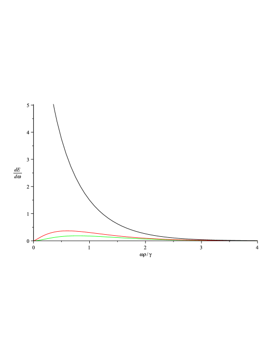
Figure 1: The spectral distribution of scalar (green), electromagnetic (red) and gravitational (black) radiation under gravitational scattering for $\gamma=1000$.

Consider now for comparison gravitational radiation under collision mediated by non-gravitational forces. Let both particles be charged (with $e_{1}$ and $e_{2}$ correspondingly) with large charge to mass ratio, so their gravitational interaction can be neglected. Then in the lowest in $G$ approximation $g_{{\mu\nu}}=\eta_{{\mu\nu}},\ S_{{\mu\nu}}=0$, and $\tau_{{\mu\nu}}=T_{{\mu\nu}}+_{F}T_{{\mu\nu}}$, where ${}_{F}T_{{\mu\nu}}$ is the energy-momentum tensor of the electromagnetic field. Calculations shows that with the same accuracy

$$T_{1}^{{\mu\nu}}(k)=\frac{2e_{1}e_{2}m_{2}^{2}}{I^{3}}e^{ik\Delta}\biggl{\{} -\biggl{(}(p_{1}p_{2})+m_{1}m_{2}\frac{z_{2}}{z_{1}}\biggr{)}K_{0}(z_{1})p_{1}^{\mu}p_{1}^{\nu}+m_{1}^{2}K_{0}(z_{1})(p_{1}^{\mu}p_{2}^{\nu}+p_{1}^{\nu}p_{2}^{\mu})-$$

$$-i(k\Delta)(p_{1}p_{2})\frac{K_{1}(z_{1})}{z_{1}}p_{1}^{\mu}p_{1}^{\nu}+i(kp_{1})(p_{1}p_{2})\frac{K_{1}(z_{1})}{z_{1}}(p_{1}^{\mu}\Delta^{\nu}+p_{1}^{\nu}\Delta^{\mu})\biggr{\}}\ ,$$ (99)

$$T_{2}^{{\mu\nu}}(k)=e^{ik\Delta}T_{1}^{\mu\nu^{*}}(1\leftrightarrow 2)\ ,$$

$${}_{F}T^{{\mu\nu}}(k) =2e_{1}e_{2}e^{ik\Delta}\int_{0}^{1}dxe^{-ix(k\Delta)}\biggl{\{}\frac{(p_{1}p_{2})}{I}\biggl{[}z(x)K_{1}(z(x))\frac{\Delta^{\mu}\Delta^{\nu}}{-\Delta^{2}}+\frac{(m_{1}m_{2})^{2}}{I^{2}}K_{0}(z(x))\frac{p_{1}^{\mu}p_{1}^{\nu}}{m_{1}^{2}}\biggr{]}-$$

$$-\frac{(m_{1}m_{2})^{2}}{I^{2}}\biggl{(}\frac{(p_{1}p_{2})}{m_{1}m_{2}}z_{2}x+z_{1}(1-x)\biggr{)}\biggl{[}\frac{(p_{1}p_{2})}{I}\biggl{(}\frac{(p_{1}p_{2})}{m_{1}m_{2}}z_{2}x+z_{1}(1-x)\biggr{)}-\frac{I}{m_{1}m_{2}}z_{2}\biggr{]}\frac{K_{1}}{z(x)}\frac{p_{1}^{\mu}p_{2}^{\nu}}{m_{1}^{2}}+$$

$$+i\frac{m_{1}m_{2}}{I}\biggl{[}\frac{(p_{1}p_{2})}{I}\biggl{(}\frac{(p_{1}p_{2})}{m_{1}m_{2}}z_{2}x+z_{1}(1-x)\biggr{)}-\frac{I}{2m_{1}m_{2}}z_{2}\biggr{]}K_{0}\biggl{(}\frac{\Delta^{\mu}}{\sqrt{-\Delta^{2}}}\frac{p_{1}^{\nu}}{m_{1}}+\frac{\Delta^{\nu}}{\sqrt{-\Delta^{2}}}\frac{p_{1}^{\mu}}{m_{1}}\biggr{)}\biggr{\}}\ ,$$ (100)

and in the chosen gauge the contribution form $T_{2}^{{\mu\nu}}$ is zero. For $\gamma\gg 1$ in the frequency region $\omega\ll\rho^{-1}$ one obtains the results (96,97), in which the gravitational deflection angle should be replaced by the electromagnetic one $4Gm_{1}m_{2}\gamma\rightarrow 2e_{1}e_{2}$.

For $\omega\geqslant\rho^{-1}$ the non-locality of the source due to presence of the term ${}_{F}T^{{\mu\nu}}$ leads to destructive interference. Like in the above cases of the gravitational interaction the non-local source ${}_{F}T^{{\mu\nu}}$ gives rise to two impulses of different duration, one of which comes to the observation point in the counterphase with the one due to $T^{{\mu\nu}}$. But contrary to the case of gravitational interaction, the contribution of $T^{{\mu\nu}}$ is canceled only partially. As a result, the spectral-angular distribution for $\omega\geqslant\rho^{-1}$ and $\gamma\gg 1$will be

$$\frac{d^{2}E_{gr}}{d\omega d\cos\theta}=\frac{2G(e_{1}e_{2})^{2}}{\pi}\omega^{2}K_{1}^{2}(\omega\rho\delta)\sin^{2}\theta\biggl{(}1-\frac{\sin^{2}\theta}{2\gamma^{2}\delta^{2}}\biggr{)}\ .$$ (101)

In the leading in $\gamma$ order we obtain

$$\frac{dE_{gr}}{d\omega}=\frac{4G(e_{1}e_{2})^{2}}{\pi\rho^{2}}z\int_{z}^{\infty}dxK_{1}^{2}(x)\biggl{(}\frac{4z}{x}-\frac{2z^{2}}{x^{2}}-3+\frac{x}{z}\biggr{)}$$ (102)

which has the following asymptotic behavior for $\rho^{-1}\leq\omega\ll\gamma^{2}/\rho$

$$\frac{dE_{gr}}{d\omega}=\frac{4G(e_{1}e_{2})^{2}}{\pi\rho^{2}}\ln\frac{4\gamma^{2}}{e^{C}\omega\rho}\ ,$$ (103)

for $\omega\gg\gamma^{2}/\rho$

$$\frac{dE_{gr}}{d\omega}=\frac{G(e_{1}e_{2})^{2}}{\rho^{2}}\biggl{(}\frac{\gamma^{2}}{\omega\rho}\biggr{)}e^{-\frac{\omega\rho}{\gamma^{2}}}\ .$$ (104)

The total energy loss is

$$\Delta E_{gr}=(\pi/4)\gamma^{2}G(e_{1}e_{2})^{2}/\rho^{3}\ .$$ (105)

The result (105) coincides with that of Pe3 .

The spectral distribution of gravitational radiation in two considered cases has the following distinctive features. For $\omega\ll\rho^{-1}$ it weakly depends on frequency and for the fixed deviation angle depends on the energy as $\gamma^{2}\ln 2\gamma$. For the frequencies $\rho^{-1}\leq\omega\ll\omega_{cr}$ the spectrum falls off logarithmically, while for $\omega\gg\omega_{cr}$ exponentially. But if for the electromagnetic interaction $\omega_{cr}^{em}=2\gamma^{2}/\rho$, for gravitational interaction $\omega_{cr}^{gr}=\gamma/\rho$. Also, for the same scattering angle the total radiated energy for electromagnetic interaction the radiative loss is $\gamma$ larger that for gravitational interaction.

VI Low frequency limit

For $\omega\rightarrow 0$ the spectral distribution does not depend on frequency and one could hope to get a correct estimate for the energy loss under collision multiplying the Eq. (67) or (93) and (94) on a suitable frequency cutoff. For radiation of the point particle in the flat space (in the case of non-gravitational interaction) the cutoff frequency in the classical spectrum is estimated kinematically as an inverse time of the formation of radiation in the given direction and it is given by $\omega_{cr}^{em}\sim\gamma^{2}/\rho$. In the gravitational case a similar estimate is $\omega_{cr}^{gr}\sim\gamma/\rho$ which is confirmed by an accurate calculation. Now, it can be easily seen that the low frequency approximation gives a correct estimate of the total radiated energy in the electromagnetic case, but gives an wrong factor $\ln 2\gamma$ in the gravitational case. The reason of this discrepancy lies in the fact that the fall-off in the spectral distribution in the gravitational case corresponds not to the frequency $\omega_{cr}$, as it is assumed in the low-frequency approach, but to $\omega\sim\rho^{-1}$ (see (96) and (103)). Logarithmic fall-off in the high frequency region $\omega\geqslant\rho^{-1}$ cancels an extra logarithmic factor. This explains the difference between our result (98) and that of Sm1 ; Sm2 .

VII Method of virtual gravitons

The spectral density of the wave packet of equivalent gravitons imitating the gravitational field of the ultrarelativistic particle is given by

$$I_{gr}(\omega,\rho)=G(m_{2}/\pi\rho)^{2}(\omega\rho/\gamma)^{2}K_{2}^{2}(\omega\rho/\gamma)$$ (106)

(this results differs from that of the ref. MaNu by a numerical factor). The spectrum diverges for $\omega\rightarrow 0$. This means that it can be applied only for sufficiently high frequencies. Applying this spectrum to compute bremsstrahlung (electromagnetic or gravitational) under scattering of the fast particle on the fixed center one has to introduce the frequency cutoff. The results differ from those obtained in this paper by a factor $\ln 2\gamma$. Thus, contrary to the electromagnetic case, where method of virtual quanta gives the correct answer in the ultrarelativistic limit, in the gravitational case this method fails. The reason is that the spectrum of virtual gravitons describes correctly the frequency range $\omega\gg\gamma/\rho$, which, as we have seen, is negligible in the total radiation due to non-locality of the effective radiation sources. Indeed, let us consider radiation in the forward direction. For $\theta=0$ the integral over the Feynman parameter can be computed exactly and we obtain

$$\left.\frac{d^{2}E_{gr}}{d\omega d\Omega}\right|_{\theta=0}=\frac{G^{3}(m_{1}m_{2})^{2}}{\pi^{2}\gamma^{2}}\omega^{2}\biggl{[}K_{2}(z_{1})-\biggl{(}\frac{z_{2}}{z_{1}}\biggr{)}^{2}K_{1}(z_{2})\biggr{]}^{2}\ .$$ (107)

At the same time the equivalent gravitons approach gives

$$\left.\frac{d^{2}E_{gr}}{d\omega d\Omega}\right|_{\theta=0}=\frac{G^{3}(m_{1}m_{2})^{2}}{\pi^{2}\gamma^{2}}\omega^{2}K_{2}^{2}(z_{1})\ .$$ (108)

One can see that the expressions (107) and (108) are compatible only for $\omega\gg\gamma/\rho$.

VIII Conclusions

We have presented Lorentz-covariant perturbation approach in General Relativity using the momentum space formulation similar to quantum field theory perturbation theory. The method consists in solving particles equations of motion and the field equations iteratively in terms of the gravitational coupling constant. Gravitational radiation arises in the second order approximation. In terms of the flat space metric the source of the D’Alembert equation for the second order metric perturbation is non-local and contains the contribution from gravitational stresses computed in the first order. This non-locality results in $\gamma$ times lower frequency cutoff as compared to the case of non-gravitational interaction. For this reason the method of virtual gravitons is not applicable for gravitational scattering of ultrarelativistic particles. The total energy loss in the rest frame of one of the particles is proportional to the third order of $\gamma$. Radiation from two colliding bodies looks as a collective effect, contributions form each of them can not be separated in a gauge independent way.

References

(1)D.V. Gal’tsov, Yu.V. Grats, A.A. Matiukhin,