Spin spirals in ordered and disordered solids

Abstract

A scheme to calculate the electronic structure of systems having a spiral magnetic structure is presented. The approach is based on the KKR (Korringa-Kohn-Rostoker) Green’s function formalism which allows in combination with CPA (Coherent Potential Approximation) alloy theory to deal with chemically disordered materials. It is applied to the magnetic random alloys Fe_xNi_1-x, Fe_xCo_1-x and Fe_xMn_1-x. For these systems the stability of their magnetic structure was analyzed. For Fe_xNi_1-x the spin stiffness for was determined as a function of concentration that was found in satisfying agreement with experiment. Performing spin spiral calculations the longitudinal momentum-dependent magnetic susceptibility was calculated for pure elemental systems (Cr, Ni) being in non-magnetic state as well as for random alloys (Ag_xPt_1-x). The obtained susceptibility was used to analyze the stability of the paramagnetic state of these systems.

I Introduction

The use of symmetry properties of solids for calculations of their electronic structure is a very efficient way to reduce the computational effort required for the solution of the problem. In particular, the single-particle electronic states of paramagnetic or collinear magnetic infinite solids can be effectively found by solving the corresponding Kohn-Sham-Dirac equation making use of the Bloch theorem. Dealing with systems exhibiting non-collinear magnetic structure, the electronic structure problem becomes much more complicated because of broken symmetry (in general, both translational and rotational), leading to an increase of the unit cell of a system and a corresponding increase of the required computational effort.

Sandratskii introduced an approach that allows to calculate the electronic structure of systems with spiral magnetic structures in an efficient way Sandratskii (1986, 1991). This approach is based on the symmetry properties of spin spiral structures as investigated by Brinkman and Elliot Brinkman and Elliot (1966a, b) and Herring Herring (3000) and allows to deal with long-period non-collinear magnetic structures avoiding the use of big unit cells in electronic structure calculations Sandratskii (1998). This makes it an efficient tool for the analysis of the stability of various non-collinear magnetic structures with different translation period, as for example demonstrated by Mryasov et al. Mryasov et al. (1991) for the investigation of the magnetic structure of fcc Fe.

In the case of systems with a collinear magnetic structure as a ground state spin spirals can be treated as transverse spin fluctuations in the adiabatic approximation. The energy dispersion of such fluctuations $\Delta E(\vec{q})$ gives access to the spin stiffness and exchange coupling constants of a system and in this way to the spin excitation spectrum as well as finite temperature magnetism Rosengaard and Johansson (1997); Halilov et al. (1998); Kübler (2000). An important feature of spin spiral calculations is that they account for longitudinal fluctuations of the magnetic moment. This leads to more reliable results for $\Delta E(\vec{q})$ compared to those obtained using the non-self consistent force-theorem approach.

As was pointed out by Sandratskii and Kübler Sandratskii and Kübler (1992) the technique for spin spiral calculations can be used for calculations of the static ($\omega=0$) momentum-resolved longitudinal magnetic susceptibility. Untill now only few corresponding ab-initio calculations have been presented in the literature. In most cases the static $q$-dependent magnetic susceptibility was calculated using perturbation theory Staunton et al. (2000) or performing super-cell calculations Jarlborg (1986). The spin spiral method, on the other hand, allows to perform self-consistent calculations of the magnetic susceptibility avoiding the super-cell concept Sandratskii and Kübler (1992).

All spin spiral calculations were done so far using the ASW Sandratskii and Guletskii (1986); Uhl et al. (1994); Kübler (2000) or LMTO Mryasov et al. (1991); Halilov et al. (1998) band structure methods. These methods use Bloch-function basis sets to represent the solution of the Kohn-Sham equation and for that reason are restricted to ordered materials concerning then application. Use of multiple scattering theory in combination with CPA (Coherent Potential Approximation) alloy theory, on the other hand, substantially extends the variety of materials which can be investigated by giving access to systems without chemical order. Here we present the implementation of spin spiral approach within the Korringa-Kohn-Rostoker (KKR) Green’s function band structure method Ebert (2000). We will show results of calculations for different systems focusing on disordered alloys.

II Theoretical background

When dealing with the electronic structure of solid state systems having a spiral magnetic structure rotations can be applied independently to the spin and spatial parts of the electronic wave function if spin-orbit coupling (SOC) is neglected. Using a spin-diagonal form of the exchange-correlation potential in the local frame of reference of an atom site, the Kohn-Sham equation for the spinor wavefuction $\psi(\vec{r})$ can be written in the form:

$$\left[-\nabla^{2}\left(\begin{array}[]{rr}1&0\\ 0&1\end{array}\right)+\sum_{n\nu}U_{n\nu}^{\dagger}(\theta_{\nu},\phi_{\nu})\left(\begin{array}[]{rr}V_{n\nu}^{+}(\vec{r})&0\\ 0&V_{n\nu}^{-}(\vec{r})\end{array}\right)U_{n\nu}(\theta_{\nu},\phi_{\nu})\right]\psi(\vec{r})=E\psi(\vec{r})\;.$$ (1)

Here $\vec{r}_{\nu}$ denotes a position of an atom in a unit cell, $\vec{R}_{n}$ is a Bravais lattice vector and $U_{n\nu}$ is a spin transformation matrix that connects the global frame of reference of the crystal to the local frame of the atom site at $\vec{r}_{\nu}+\vec{R}_{n}$ that has its magnetic moment tilted away from the global z-direction. The transformation $U_{n\nu}$ is characterized by the Euler angles $\theta_{n,\nu}$ and $\phi_{n,\nu}$ as is is shown in Fig. 1 for the case of a spin spiral.

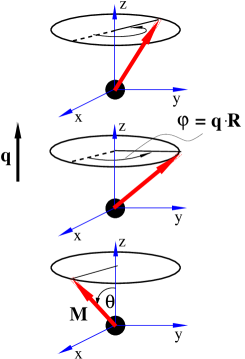
Figure 1: Geometry of a spin spiral with the wave vector $\vec{q}$ along the z-direction.

As was shown by Sandratskii, considering a spin spiral structure, Eq. (1) can be easily dealt with using the properties of spin space groups (SSG) Brinkman and Elliot (1966a, b); Herring (3000) allowing independent transformations within the spin and space sub-spaces. The spin spirals characterized by the wave vector $\vec{q}$ angles $\theta_{\nu}$ and $\phi_{\nu}$ are represented by the expression:

$$\vec{m}_{n}^{\nu}=m^{\nu}\,[\mbox{cos}(\vec{q}\cdot\vec{R}_{n}+\phi_{\nu})\mbox{sin}\theta_{\nu},\mbox{sin}(\vec{q}\cdot\vec{R}_{n}+\phi_{\nu})\mbox{sin}\theta_{\nu},\mbox{cos}\theta_{\nu}]$$

defining the spin direction at every site $(n,\nu)$ of the lattice with $m^{\nu}$ the magnitude of the magnetic moment on site $\nu$ within the unit cell. Assuming a collinear alignment of the spin density within the atomic cell at $(n,\nu)$, it’s natural to use a local frame of reference with its z-axis oriented along $\vec{m}_{n}^{\nu}$. The corresponding transformation matrices $U_{n\nu}$ occurring in Eq.  (1) can be written as a product of two independent rotation matrices $U^{\vec{q}}_{n\nu}=U_{n}(\theta_{\nu},\phi_{\nu},\vec{q})=U_{\nu}(\theta_{\nu},\phi_{\nu})U_{\vec{q}\vec{R}_{n}}$ where the matrix $U_{\vec{q}\vec{R}_{n}}$ depends only on the translation vector $\vec{R}_{n}$:Sandratskii (1986, 1991)

$$U_{n}(\theta_{\nu},\phi_{\nu},\vec{q})=$$ (8)

$$= \left(\begin{array}[]{rr}\cos\frac{\theta_{\nu}}{2}&\sin\frac{\theta_{\nu}}{2}\\ -\sin\frac{\theta_{\nu}}{2}&\cos\frac{\theta_{\nu}}{2}\end{array}\right)\left(\begin{array}[]{rr}e^{\frac{i}{2}\phi_{\nu}}&0\\ 0&e^{-\frac{i}{2}\phi_{\nu}}\end{array}\right)\left(\begin{array}[]{rr}e^{\frac{i}{2}(\vec{q}\cdot\vec{R_{n}})}&0\\ 0&e^{-\frac{i}{2}(\vec{q}\cdot\vec{R_{n}})}\end{array}\right)=U_{\nu}\,U_{\vec{q}\vec{R}_{n}}\;.$$

Instead of solving the Kohn-Sham Eq. (1) for the eigen functions and values the electronic structure can be represented in terms of the corresponding Green’s function. Within multiple scattering theory the Green’s function is represented in real space by the scattering path operator $\tilde{\underline{\tau}}^{nn^{\prime}}$ together with the regular $Z^{n}_{\Lambda_{1}}(\vec{r},E)$ and irregular $J^{n}_{\Lambda_{1}}(\vec{r},E)$ solutions of the single-site Kohn-Sham equation referring to the local frame of reference:

$$G^{+}(\vec{r},\vec{r}\;^{\prime},E) = \sum_{\Lambda_{1}\Lambda_{2}}Z^{n}_{\Lambda_{1}}(\vec{r},E){\tau}^{nn^{\prime}}_{\Lambda_{1}\Lambda_{2}}(E)Z^{n^{\prime}\times}_{\Lambda_{2}}(\vec{r}\;^{\prime},E)$$ (9)

$$-\sum_{\Lambda_{1}}\Big{[}Z^{n}_{\Lambda_{1}}(\vec{r},E)J^{n\times}_{\Lambda_{1}}(\vec{r}\;^{\prime},E)\Theta(r^{\prime}-r)$$

$$\qquad\quad J^{n}_{\Lambda_{1}}(\vec{r},E)Z^{n\times}_{\Lambda_{1}}(\vec{r}\;^{\prime},E)\Theta(r-r^{\prime})\Big{]}\delta_{nn^{\prime}}\;.$$

The scattering path operator is defined by its equation of motion:

$${\underline{\tau}}^{n\nu\,n^{\prime}\nu^{\prime}} = {\underline{t}}^{n\nu}\delta_{n\nu\,n^{\prime}\nu^{\prime}}+{t}^{n\nu}{\sum_{kp}}^{\prime}{\underline{G}}^{nq\,m\mu}\,{\underline{\tau}}^{m\mu\,n^{\prime}\nu^{\prime}}\;,$$ (10)

where ${t}^{n\nu}$ and ${\underline{G}}^{nq\,m\mu}$ are the single-site t-matrix and free-electron propagator, respectively, that are all expressed with respect to a common global frame of reference. Eq. (10) has the formal solution

$$\underline{\underline{{\tau}}} = \left[\underline{\underline{{t}}}^{-1}-\underline{\underline{{G}}}\right]^{-1}\;.$$ (11)

In Eqs. (10) and (11) the underline indicates matrices in the $(l,m)$ representation while double underline indicates super-matrices including the site index. In the case of a collinear magnetic structure the local and global frames of reference coincide. This implies that Eq. (11) gives immediately the solution with respect to the local frame of reference. For infinite systems having a regular periodic lattice a solution to Eq. (10) can be obtained by Fourier transformation instead of using the real space expression given in Eq. (11) .

For non-collinear magnetic solids with a periodic lattice structure one can solve Eq. (10) as for collinear systems but using an extended super-cell. The size of the corresponding super-cell is determined by the period of magnetic structure. All atoms within the cell are in general inequivalent and have their own local frame of reference. Therefore super-cell calculations can be rather time consuming in particular for magnetic structures having a long period.

However, as pointed by various authors Brinkman and Elliot (1966a, b); Herring (3000) use of symmetry allows to simplify the problem substantially. Spiral magnetic structures transform according to the group of generalized translations that are characterized by the wave vector $\vec{q}$ and represented by the matrices $U_{\vec{q}\vec{R}_{n}}$ (Eq. (8)). This implies in particular that the matrices $U_{\vec{q}\vec{R}_{n}}$ allow to express the single-site t-matrix ${t}^{n\nu}$ at site $({n\nu})$ to that at site $({0\nu})$. This symmetry property allows to write the scattering path operator referring the global frame of reference as follows:

$$\tau^{n\nu\,n^{\prime}\nu^{\prime}} = t^{n\nu}\delta_{n\nu\,n^{\prime}\nu^{\prime}}+t^{n\nu}{\sum_{m\mu}}^{\prime}G^{n\nu\,m\mu}\tau^{m\mu\,n^{\prime}\nu^{\prime}}$$ (12)

$$= U_{n\nu}^{\vec{q}\,\dagger}\tilde{t}^{n\nu}U_{n\nu}^{\vec{q}}\delta_{n\nu\,n^{\prime}\nu^{\prime}}+U_{n\nu}^{\vec{q}\,\dagger}\tilde{t}^{n\nu}U_{n\nu}^{\vec{q}}{\sum_{m\mu}}^{\prime}G^{n\nu\,m\mu}\tau^{m\mu\,n^{\prime}\nu^{\prime}}\;.$$

This allows to find the scattering path operator and from this the Green’s function in the local frame of reference of the each atom, solving the equation

$$\tilde{\underline{\tau}}^{n\nu\,n^{\prime}\nu^{\prime}} = U_{n\nu}^{\vec{q}}\underline{\tau}^{n\nu\,n^{\prime}\nu^{\prime}}U_{n^{\prime}\nu^{\prime}}^{\vec{q}\,\dagger}$$ (13)

$$= \tilde{\underline{t}}^{n\nu}\delta_{n\nu\,n^{\prime}\nu^{\prime}}+\tilde{\underline{t}}^{n\nu}{\sum_{m\mu}}^{\prime}U_{n\nu}^{\vec{q}}\underline{G}^{n\nu\,m\mu}U_{m\mu}^{\vec{q}\,\dagger}\,U_{m\mu}^{\vec{q}}\underline{\tau}^{m\mu\,n^{\prime}\nu^{\prime}}U_{n^{\prime}\nu^{\prime}}^{\vec{q}\,\dagger}$$

$$= \tilde{\underline{t}}^{\nu}\delta_{n\nu\,n^{\prime}\nu^{\prime}}+\tilde{\underline{t}}^{\nu}{\sum_{m\mu}}^{\prime}\underbrace{U_{n\nu}^{\vec{q}}\underline{G}^{n\nu\,m\mu}U_{m\mu}^{\vec{q}\,\dagger}}_{\tilde{\underline{G}}^{n\nu\,m\mu}}\,\underbrace{U_{m\mu}^{\vec{q}}\underline{\tau}^{m\mu\,n^{\prime}\nu^{\prime}}U_{n^{\prime}\nu^{\prime}}^{\vec{q}\,\dagger}}_{\tilde{\underline{\tau}}^{m\mu\,n^{\prime}\nu^{\prime}}}\;,$$ (14)

where the tilde indicates matrices which refer to the local frame of reference.

In the last line of Eq.  (14) use has been made that the single-site t-matrices $\tilde{\underline{t}}^{n\nu}$ do not depend on the lattice index $n$ but only on the site index $\nu$ in the unit cell. As a consequence, the multiple scattering problem can be solved as for the case of collinear magnetic structures by Fourier transformation of the equation of motion for the scattering path operator. This leads to its representation in reciprocal space according to:

$$\underline{\underline{\tilde{\tau}}}(\vec{k},E) = \left[\underline{\underline{\tilde{t}}}^{-1}(E)-\underline{\underline{\tilde{G}}}(\vec{k})\right]^{-1}\;.$$ (15)

The structural Green’s function referring to the local frame of reference can be determined as follows:

$$\tilde{\underline{G}}^{\nu\nu^{\prime}}(\vec{k}) = \frac{1}{N}\sum_{nn^{\prime}}e^{-i\vec{k}\cdot(\vec{R}_{n}-\vec{R}_{n^{\prime}})}\tilde{\underline{G}}^{n\nu\,n^{\prime}\nu^{\prime}}$$ (18)

$$= \frac{1}{N}\sum_{nn^{\prime}}e^{-i\vec{k}\cdot(\vec{R}_{n}-\vec{R}_{n^{\prime}})}U_{n\nu}^{\vec{q}}\underline{G}^{n\nu\,n^{\prime}\nu^{\prime}}U_{n^{\prime}\nu^{\prime}}^{\vec{q}\,\dagger}$$

$$= U_{\nu}\left(\begin{array}[]{rr}\underline{G}^{\nu\nu^{\prime}}(\vec{k}-\frac{1}{2}\vec{q})&0\\ 0&\underline{G}^{\nu\nu^{\prime}}(\vec{k}+\frac{1}{2}\vec{q})\end{array}\right)U_{\nu^{\prime}}^{\dagger}$$

$$= U_{\nu}\,\underline{G}^{\nu\nu^{\prime}}_{\vec{q}}(\vec{k})\,U_{\nu^{\prime}}^{\dagger}\;.$$ (19)

Here $\underline{G}^{\nu\nu^{\prime}}(\vec{k})$ is a structural Green’s function for one spin channel represented in the global frame of reference.

The charge distribution within the central unit cell $n=0$ is determined by the cell-diagonal scattering path operator $\tilde{\underline{\underline{\tau}}}^{00}$ which can be found by the Brillouin zone integral

$$\tilde{\underline{\underline{\tau}}}^{00} = \frac{1}{\Omega_{BZ}}\int_{\Omega_{BZ}}d^{3}k\left[\tilde{\underline{\underline{t}}}^{-1}-\tilde{\underline{\underline{G}}}(\vec{k})\right]^{-1}$$ (20)

$$= U_{0}^{\dagger}\frac{1}{\Omega_{BZ}}\int_{\Omega_{BZ}}d^{3}k\left[{\underline{\underline{t}}}^{-1}-\underline{\underline{G}}_{\vec{q}}(\vec{k})\right]^{-1}U_{0}$$

$$= U_{0}^{\dagger}\underline{\underline{\tau}}^{00}U_{0}\;,$$

where $U_{0}$ is the transformation matrix diagonalising the potentials as well as $t$-matrices with respect to spin within the central unit cell.

To perform calculations for disordered alloys the CPA (Coherent Potential Approximation) alloy theory Matsumoto et al. (1990); Butler (1985) is used. In the case of a spin spiral system the CPA medium is represented in the global frame of reference by the effective single-site scattering matrix $\underline{t}^{C}$ and the scattering path operator obtained from the expression:

$$\underline{\underline{\tau}}^{00\rm,C}(E)=\frac{1}{\Omega_{\rm BZ}}\int_{\Omega_{\rm BZ}}d^{3}k\left[(\underline{\underline{t}}^{\rm C}(E))^{-1}-\underline{\underline{G}}(\vec{k},E)\right]^{-1}\;.$$ (21)

The corresponding element projected scattering path operators are obtained from these via:

$$\underline{\underline{\tau}}^{00,\alpha} \,=\,\underline{\underline{\tau}}^{00,\rm C}\,\underline{\underline{D}}^{\alpha}\,,$$ (22)

with

$$\underline{\underline{D}}^{\alpha} \,=\,\left[\underline{\underline{1}}+\left[(\underline{\underline{t}}^{\alpha})^{-1}-(\underline{\underline{t}}^{\rm C})^{-1}\right]\underline{\underline{\tau}}^{00,\rm C}\right]^{-1}\,.$$ (23)

The approach developed for calculations of non-collinear spin spiral structures can be used for investigations on the longitudinal magnetic susceptibility as a function of the wave vector $\vec{q}$ Sandratskii and Kübler (1992). This approach allows to avoid the use of perturbation theory and can be applied to magnetic as well as non-magnetic systems. In the following we focus on materials in their non-magnetic state which may exhibit paramagnetism (Ag_xPt_1-x), ferromagnetism (Ni) or antiferromagnetism (Cr) in their ground state. For this purpose we specify a spiral external magnetic field to be perpendicular to the direction of the wave vector $\vec{q}$ (i.e. $\theta=90^{o}$):

$$\vec{h}(\vec{r})=h_{0}[\mbox{cos}(\vec{q}\cdot\vec{R}_{n}),\mbox{sin}(\vec{q}\cdot\vec{R}_{n}),0]\;.$$

In this case is the potential energy term in the Kohn-Sham equation (see Eq. (1)) is given by:

$$\left[\sum_{n\nu}U_{n\nu}^{\dagger}(\theta_{\nu},\phi_{\nu})\left(\begin{array}[]{cc}V_{n\nu}(\vec{r})-B_{n}^{ext}-\Delta B_{n}^{xc}(\vec{r})&0\\ 0&V_{n\nu}(\vec{r})+B_{n}^{ext}+\Delta B_{n}^{xc}(\vec{r})\end{array}\right)U_{n\nu}(\theta_{\nu},\phi_{\nu})\right]\;.$$ (24)

A self-consistent calculation based on Eq. (24) gives the spin magnetic moment induced by the external magnetic field. The $\vec{q}$-dependent external magnetic field should be taken small enough to be considered as a perturbation. In this case, assuming a linear response to be the leading term of the response function the corresponding magnetic susceptibility can be derived from the expression

$$\chi(\vec{q}) = \frac{m_{ind}(\vec{q})}{h_{0}}\;.$$ (25)

Suppressing the spin-dependent part of the exchange-correlation potential ($\Delta B_{n}^{xc}(\vec{r})=0$), one can calculate the unenhanced spin susceptibility $\chi^{0}(\vec{q})$. Otherwise, Eq. (25) gives the enhanced longitudinal magnetic susceptibility $\chi(\vec{q})$, represented in linear response theory for uniform system by the expression

$$\chi(\vec{q}) = \frac{\chi^{0}(\vec{q})}{1-I(\vec{q})\chi^{0}(\vec{q})}\;,$$ (26)

with $I(\vec{q})$ the exchange integral responsible for the enhancement of the magnetic susceptibility (see, for example, Kübler (2000); Deng (2001)). In case of a paramagnetic ground state the magnetic susceptibility $\chi(\vec{q})$ is positive for all values of $\vec{q}$. For other cases the denominator in the Eq. (26) may become zero or even negative. This singular behavior of the susceptibility obviously indicates an instability of the paramagnetic state towards a transition to spontaneous formation of ferro- or anti-ferronagnetic order.

III Results

III.1 Spin spiral structure in alloys

In the following several applications of the scheme introduced above are presented that focus on disordered alloys to demonstrate the flexibility of the multiple scattering formalism when dealing with spin spiral systems. Corresponding calculations have been performed for alloys having fcc (Fe_xNi_1-x and Fe_xMn_1-x) and bcc (Fe_xCo_1-x) lattice structure.

For all calculations the angle $\theta$ has been chosen to be $90^{o}$. For this spin geometry, the spin spiral with $\vec{q}=\frac{\pi}{a}(0,0,1)$ corresponds to a spin configuration where the first neighbor atoms in the (001) direction have an anti-parallel (AFM) spin alignment, while $\vec{q}=\vec{0}$ implies a parallel (FM) orientation.

III.1.1 The disordered alloy system Fe_xNi_1-x

Fig. 2a shows the energy of the disordered Fe_xNi_1-x alloy system with a spin spiral structure as a function of the wave vector $\vec{q}$. For all concentrations the minimum of the energy is found for $\vec{q}=\vec{0}$, implying that the ferromagnetic structure is more stable configuration than non-collinear structures characterized by wave vectors along the (001) direction.

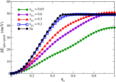
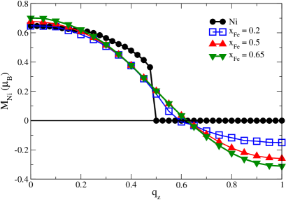
Figure 2: a) The energy of spin spiral magnetic structure in Fe_xNi_1-x alloys and b) local magnetic moments on Ni atoms as a function of the wave vector $\vec{q}=\frac{\pi}{a}(0,0,q_{z})$.

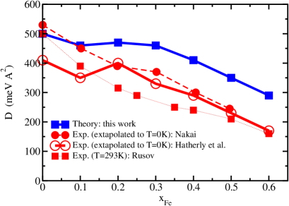
Figure 3: Spin stiffness constant of Fe_xNi_1-x alloys as a function of the concentration in comparison with experiment: Nakai Nakai (1983) (full circles), Hatherly et al. Hatherly et al. (1964) (open circles), Rusov Rusov (1967) (full squares).

As can be seen from Fig. 2b, the local magnetic moment of Ni in pure Ni drops down to $m=0$ at the wave vector $\vec{q}_{c}\approx\frac{\pi}{a}(0,0,0.5)$ and the system becomes paramagnetic. In terms of the Stoner theory of ferromagnetism (see, e.g.  Ref. Kübler, 2000) this means that the criterium for the instability of the paramagnetic state is satisfied only for small wave vectors, while above $\vec{q}_{c}$ the paramagnetic (PM) state should be the most stable state of the system. The criterion for the instability of the PM state will be discussed below in more detail.

Adding only small amounts of Fe to Ni leads obviously to a nonzero magnetic moment per unit cell at all values of wave vector $\vec{q}$. This is caused by the large magnetic moment of Fe which depends only slightly on the wave vector. Fig. 2b shows that the Ni magnetic moment in contrast to that of Fe, varies rather rapidly with increasing wave vector and changes sign at $\vec{q}\approx\frac{\pi}{a}(0,0,0.6)$. This means that in the vicinity of the ground state of the alloys ($\vec{q}=\vec{0}$) the magnetic moments of Fe and Ni atoms prefer to have parallel alignment, while close to $\vec{q}=\frac{\pi}{a}(0,0,1)$ (AFM structure along (0,0,1) direction) the more favorable orientation of the Fe and Ni moments is anti-parallel (AP). Nevertheless, even for small Fe concentrations, the total magnetic moment is determined by the dominating moment of Fe. As a result, the alloy system exhibits effectively a ferromagnetic behavior for all wave vectors, as one can see in Fig. 2.

The energy difference between the spin spiral states with $\vec{q}=\vec{0}$ and $\vec{q}=\frac{\pi}{a}(0,0,1)$ remains almost unchanged up to the Fe concentration $x_{Fe}\approx 0.6$, and changes nearly by 20 % when approaching $x_{Fe}\approx 0.65$. On the other hand, the spin-stiffness constant deduced from the energy dispersion curves decreases continuously with the increase of Fe content as can be seen from Fig.  3. This figure also shows that the calculations reproduce the available experimental data for the spin-stiffness constant fairly well, although they seem to be slightly to high. This difference can be partially attributed to the conditions of the experiment as e.g. polycrystallinity of the samples and a finite temperature.

III.1.2 The disordered alloy Fe_0.5Co_0.5

The change of sign of the magnetic moment observed for Fe_xNi_1-x alloys for one of the alloy components upon variation of the wave vector becomes even more pronounced in bcc Fe_0.5Co_0.5 and fcc Fe_0.5Mn_0.5 alloys. Disordered bcc Fe_0.5Co_0.5 has a ferromagnetic ground state. The spin spiral energy shown in Fig. 4a increases with wave vector confirming the stability of the FM state.

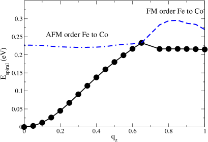
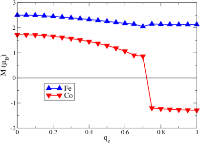
Figure 4: a) the energy of spin spiral magnetic structure in Fe_0.5Co_0.5 calculated for the wave vector $\vec{q}=\frac{\pi}{a}(0,0,q_{z})$ along [001] direction; b) local magnetic moments on Fe and Co atoms separately, as a function of wave vector of spin spirals.

As can be seen from Fig. 4b, around $\vec{q}=\vec{0}$ the individual Fe and Co moments are aligned parallel with respect to each other. However, after crossing $\vec{q}_{c}\approx\frac{\pi}{a}(0,0,0.7)$, the total magnetic moment jumps from $m=1.46\mu_{B}$ to $m=0.47\mu_{B}$ due to a change of the sign of the Co magnetic moment with respect to that of the dominating Fe moment. As Fig. 4b shows, the dispersion of the spin spiral energy for the anti-parallel configuration gets very weak up to $\vec{q}\approx\frac{\pi}{a}(0,0,1)$. To estimate the energy of the spin spirals for the non-equilibrium configurations, i.e. anti-parallel for $\vec{q}_{c}<\frac{\pi}{a}(0,0,0.7)$ and parallel for $\vec{q}_{c}>\frac{\pi}{a}(0,0,0.7)$, respectively, frozen potential calculations have been performed. The corresponding results are represented in Fig. 4b by dashed and dashed-dotted lines. Obviously, these results augment the two stable branches fairly will.

III.1.3 The disordered alloy Fe_0.5Mn_0.5

Fig. 5 shows the results of spin spiral calculations for Fe_0.5Mn_0.5 having a non-collinear magnetic structure as a ground state Johnson et al. (1988); Schulthess et al. (1999); Endoh and Ishikawa (1971).

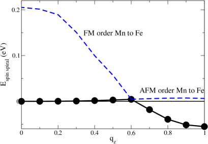
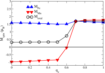
Figure 5: a) The energy of spin spiral magnetic structure in Fe_xMn_1-x alloys calculated for the wave vector $\vec{q}=\frac{\pi}{a}(0,0,q_{z})$ along [001] direction; b) local magnetic moments on Fe and Mn atoms separately, as a function of wave vector of spin spirals.

As is seen in the energy dispersion curve, Fig. 5a, the system exhibits the behavior of a FM system for wave vectors $\vec{q}$ up to $\vec{q}_{c}\approx\frac{\pi}{a}(0,0,0.6)$. In this wave vector region the alloy has a small average magnetic moment formed by two anti-parallel aligned magnetic moments of Fe and Mn occupying randomly the site (see Fig. 5b).

At $\vec{q}_{c}\approx\frac{\pi}{a}(0,0,0.6)$ the energy of a spin spiral reaches its maximum and the following increase of the wave vector is accompanied by a decrease in energy and an increase of the average magnetic moment. At $\vec{q}=(0,0,\frac{\pi}{a})$ the spin spiral magnetic structure reaches its energy minimum, which is about 50 meV lower than the energy of the FM state, with a parallel alignment of the magnetic moments of the alloy components.

Similar to Fe_0.5Co_0.5, these two minima of the energy – around $\vec{q}=\vec{0}$ and around $\vec{q}=(0,0,\frac{\pi}{a})$ – are formed by two crossing branches of the spin spiral dispersion relation: one corresponds to an anti-parallel alignment of the Fe and Mn magnetic moments (around the $\vec{q}=\vec{0}$) and another to their parallel alignment (around $\vec{q}=(0,0,\frac{\pi}{a})$ ), which have a crossing point at $\vec{q}\approx\frac{\pi}{a}(0,0,0.6)$.

Thus, from the analysis of the energetics of the spin spiral structures in Fe_0.5Mn_0.5, one can conclude that the system has in its magnetic ground state an anti-parallel alignment of the magnetic moments of first neighbors, no matter whether the neighboring atoms are Fe or Mn.

III.2 Spin susceptibility

In the present section we will discuss another application of the technique presented above. As was shown by Sandratskii and Kübler Sandratskii and Kübler (1992), spin spiral calculations can also be used to determine the longitudinal magnetic susceptibility $\chi$, both for magnetic and non-magnetic systems, as a function of the wave vector $\vec{q}$. This approach allows in particular to avoid the use of perturbation theory. Adding a Zeeman term to the Hamiltonian corresponding to a small external helical magnetic field allows to obtain the magnetic susceptibility from the the induced magnetic moments. For the present calculations a Zeeman splitting $h_{0}=1$ meV has been used.

The present work deals with non-magnetic systems, which have either a paramagnetic (AgPt), a ferromagnetic (Ni) or an anti/ferromagnetic (Cr) ground state. Dealing with magnetic systems being in an imposed paramagnetic state, their magnetic susceptibility gives information on an instability with respect to magnetic ordering.

III.2.1 The paramagnetic disordered alloy Ag_xPt_1-x

Fig. 6 shows the magnetic susceptibility of paramagnetic Ag_xPt_1-x alloys as a function of the wave vector $\vec{q}$  for various concentrations.

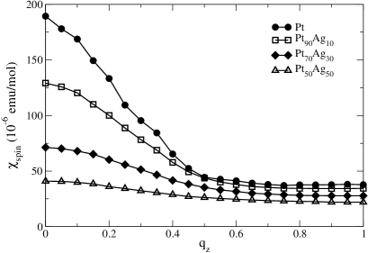
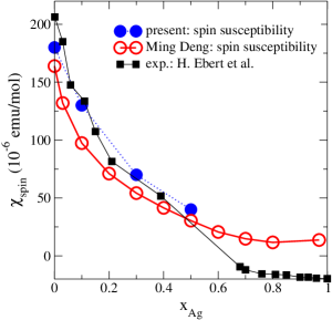
Figure 6: a) Wave-vector ($\vec{q}=\frac{\pi}{a}(0,0,q_{z})$) dependent magnetic susceptibility of the paramagnetic disordered Ag_xPt_1-x for various concentrations. b) Comparison of the present results for the susceptibility for $q=0$ with the results of Deng et al. Deng (2001) obtained via linear response theory.

The spin susceptibility of the alloys presented in Fig. 6 is composed by contributions from both components according to $\chi(\vec{q})=x\chi_{Ag}(\vec{q},x)+(1-x)\chi_{Pt}(\vec{q},x)$. For all concentrations, the increase of the wave vector for helical magnetic field is accompanied by a decrease of the response functions, as it is usually found for paramagnetic systems. The main contribution to the spin susceptibility stems from the Pt atoms. As can be seen, increasing the Ag content leads to a decrease of the magnetic susceptibility for all values of wave vector.

The present results for $\vec{q}=\vec{0}$ are compared with the total magnetic susceptibility obtained via fully relativistic linear response calculations Deng (2001). As one can see, the agreement of results obtained by the two rather different theoretical approaches is rather good. One reason for the observed deviations is the use of a finite value for the external magnetic field in the present calculations giving the magnetic susceptibility from the induced magnetic moment within the self-consistent calculations. Another reason is the neglect of spin-orbit coupling within the present calculations that usually reduces the spin susceptibility. Nevertheless, both approaches lead obviously to coherent results that are in rather satisfying agreement with experimental results Ebert et al. (1984) (full squares in Fig. 6b). Note however, that experimental results represent the total magnetic susceptibility including also the orbital contribution.

III.2.2 Pure ferromagnetic fcc Ni

The calculations performed for ferromagnetic Ni in a paramagnetic state show a behavior for the magnetic susceptibility as a function of the wave vector that is rather different from that of systems with a paramagnetic ground state as for example Ag_xPt_1-x alloys) (see Fig. 7). The paramagnetic state of Ni was simulated using the disordered local moment (DLM) Gyorffy et al. (1985) method assuming equal concentration for atoms with opposite orientation of their magnetic moments. The magnetically disordered state of Ni is characterized by a vanishing local magnetic moment and therefore the DLM method allows us to force the local magnetic moment to be zero. Fig. 7a shows the results obtained for Ni with the experimental lattice parameter $a=6.65$ a.u. At small values of the wave vector $\vec{q}$ the magnetic susceptibility is negative indicating an instability of the paramagnetic state. This is a result of the high density of states (DOS) of the 3d-electrons leading to a large value of the unenhanced magnetic susceptibility $\chi^{0}$. Accordingly, for small $\vec{q}$-vectors the Stoner condition for a magnetic instability $I(\vec{q})\chi^{0}(\vec{q})>1$ (Eq. 26) (see, e.g., Moriya (1985); Mohn (2003)) is fulfilled.

As one can see in Fig. 7, at the wave vector $\vec{q}\approx\frac{\pi}{a}(0,0,0.55)$ (for which the denominator in Eq. (26) comes to 0) the magnetic susceptibility becomes singular and the following increase of $\vec{q}$ results in a change of sign for the susceptibility from negative to positive leading to the stability of the paramagnetic state.

Fig. 7a shows also the Ni magnetic moment as a function of the wave vector $\vec{q}$ of spin spiral. As one can see, the magnitude of the goes down upon increase of $\vec{q}$ reaching $m=0$ at the critical value of the wave vector $\vec{q}_{c}$.

As is shown in Fig. 7b, a decrease of the lattice parameter leads to a decrease of the unenhanced susceptibility $\chi(\vec{q})$ due to the broadening of the energy bands of the 3d-states. This results in a decrease of the critical wave vectors $\vec{q}_{c}$ until a lattice parameter is reached for which $\vec{q}_{c}=0$. For smaller lattice parameters the ground state of Ni is the PM state.

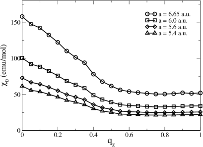
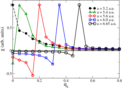
Figure 7: Wave-vector dependent spin susceptibility of paramagnetic Ni having lattice parameter $a=6.65$ a.u. together with local Ni magnetic moment as a function of wave-vector characterizing non-collinear spiral magnetic structure (a). The wave-vector dependent unenhanced (b) and enhanced (c) magnetic susceptibilities for paramagnetic Ni calculated for different lattice parameters.

III.2.3 Pure antiferromagnetic bcc Cr

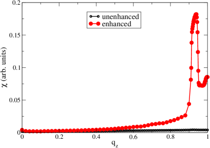
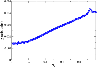
Figure 8: Wave-vector dependent enhanced (a) and unenhanced (b) spin susceptibilities of paramagnetic Cr. For comparison, the unenhanced susceptibility is plotted also at the panel (a).

Results for the non-magnetic state of Cr having the AFM structure as a ground state are shown in Fig. 8. Note that the antiferromagnetic order of Cr on the one side is a result of nearly-half filling of the d-band Moriya (1985) (similar to Mn), that should result in a commensurate AFM structure. However, Cr exhibits also an instability with respect to an incommensurate spin-density wave (SDW) with the wave vector $\vec{q}\approx\frac{\pi}{a}(0,0,0.95)$, which is a result of the Fermi surface nesting. This leads to a singularity of the magnetic susceptibility at $\vec{q}\approx\frac{\pi}{a}(0,0,0.95)$ of paramagnetic Cr. This SDW instability in Cr and the corresponding behavior of the momentum dependent magnetic susceptibility was discussed in the literature by several authors Staunton et al. (1999); Crockford and Yeung (1993); Fawcett (1988).

Our present results demonstrate that the calculation of the momentum-resolved magnetic susceptibility properly reproduce its $\vec{q}$ dependent features for Cr. The calculations have been performed for a lattice parameter $a=5.4$ a.u. which is slightly smaller than the experimental one ($a\approx 5.44$ a.u.). At this lattice parameter the PM state was found to be more stable than the AFM state. This allows us to observe the behavior of $\chi(\vec{q})$ due to the Fermi surface nesting avoiding the influence of other singularities connected to the instability around $\vec{q}=\pi/a(0,0,1)$ with respect to the AFM state.

Fig. 8b shows a monotonous increase of the unenhanced susceptibilities with increasing wave vector $\vec{q}$ reaching its maximum at $\vec{q}\approx\pi/a(0,0,0.92)$. The enhanced susceptibility, also increasing with wave vector $\vec{q}$, has a drastic increase at $\vec{q}\approx\pi/a(0,0,0.92)$ due the enhancement factor (Eq. (26)), which is associated with a singularity caused by the Fermi surface nesting mentioned above.

Here, we do not discuss the $q$ dependence of the exchange integral $I(\vec{q})$ as this was done in detail by Sandratskii and Kübler. Nevertheless, we would like to stress that this feature is taken into account within the self-consistent calculations for every wave vector. In fact this is essential for the analysis of the stability of the paramagnetic state.

IV Conclusion

A theoretical approach for electronic structure calculations on systems with spiral magnetic structures within the KKR Green’s function formalism has been presented. As has been demonstrated, by making use of symmetry, the scattering path operator can be obtained by solving the corresponding equation of motion in the reciprocal space. Compared to the case of collinear magnetic structure only the structural Green’s function to be used involves the wave vector of the spin spiral. As the KKR-formalism combined with the CPA allows to deal with chemically disordered materials, corresponding spin spiral investigations on various disordered alloys could be performed. In particular the energy of spin spirals and the behavior of the magnetic moments of the alloy components was analyzed. In addition is was shown that the approach presented can be efficiently used for the calculation of the momentum resolved longitudinal magnetic susceptibilities of pure materials as well as of disordered alloys.

V Acknowledgement

This work was supported by the DFG within the project Eb 154/20 ”Spin polarisation in Heusler alloy based spintronics systems probed by SPINAXPES”.

References

- Sandratskii (1986) L. M. Sandratskii, phys. stat. sol. (b) 135, 167 (1986).
- Sandratskii (1991) L. M. Sandratskii, J. Phys.: Condens. Matter 3, 8565 (1991).
- Brinkman and Elliot (1966a) W. F. Brinkman and R. J. Elliot, Proc. Roy. Soc. (London) A 294, 343 (1966a).
- Brinkman and Elliot (1966b) W. F. Brinkman and R. J. Elliot, J. Appl. Phys. 37, 1457 (1966b).
- Herring (3000) C. Herring, in Magnetism, edited by G. Rado and H. Suhl (Academic Press, New York, 3000), vol. IV, p. 191.
- Sandratskii (1998) L. M. Sandratskii, Adv. Phys. 47, 91 (1998).
- Mryasov et al. (1991) O. N. Mryasov, A. I. Liechtenstein, L. M. Sandratskii, and V. A. Gubanov, Journal of Physics: Condensed Matter 3, 7683 (1991).
- Halilov et al. (1998) S. V. Halilov, H. Eschrig, A. Y. Perlov, and P. M. Oppeneer, Phys. Rev. B 58, 293 (1998), URL http://link.aps.org/doi/10.1103/PhysRevB.58.293.
- Rosengaard and Johansson (1997) N. M. Rosengaard and B. Johansson, Phys. Rev. B 55, 14975 (1997).
- Kübler (2000) J. Kübler, Theory of itinerant electron magnetism (Oxford University Press, Oxford, 2000), p. 460.
- Sandratskii and Kübler (1992) L. M. Sandratskii and J. Kübler, J. Phys.: Condens. Matter 4, 6927 (1992).
- Staunton et al. (2000) J. B. Staunton, J. Poulter, B. Ginatempo, E. Bruno, and D. D. Johnson, Phys. Rev. B 62, 1075 (2000).
- Jarlborg (1986) T. Jarlborg, Solid State Commun. 57, 683 (1986).
- Sandratskii and Guletskii (1986) L. M. Sandratskii and P. G. Guletskii, J. Phys. F: Met. Phys. 16, L43 (1986).
- Uhl et al. (1994) M. Uhl, L. M. Sandratskii, and J. Kübler, Phys. Rev. B 50, 291 (1994).
- Ebert (2000) H. Ebert, in Electronic Structure and Physical Properties of Solids, edited by H. Dreyssé (Springer, Berlin, 2000), vol. 535 of Lecture Notes in Physics, p. 191.
- Matsumoto et al. (1990) M. Matsumoto, J. B. Staunton, and P. Strange, J. Phys.: Cond. Mat. 2, 8365 (1990).
- Butler (1985) W. H. Butler, Phys. Rev. B 31, 3260 (1985), URL http://link.aps.org/doi/10.1103/PhysRevB.31.3260.
- Deng (2001) M. Deng, Ph.D. thesis, University of Munich (2001).
- Nakai (1983) I. Nakai, J. Phys. Soc. Japan 52, 1781 (1983).
- Hatherly et al. (1964) M. Hatherly, K. Hirakawa, R. D. Lowde, J. F. Mallett, M. W. Stringfellow, and B. H. Torrie, Proc. Phys. Soc. (London) 84, 55 (1964).
- Rusov (1967) G. I. Rusov, Sov. Phys.-Solid State 9, 146 (1967).
- Schulthess et al. (1999) T. C. Schulthess, W. H. Butler, G. M. Stocks, S. Maat, and G. J. Mankey, J. Appl. Physics 85, 4842 (1999).
- Johnson et al. (1988) D. D. Johnson, F. J. Pinski, and G. M. Stocks, J. Appl. Phys. 63, 3490 (1988).
- Endoh and Ishikawa (1971) Y. Endoh and Y. Ishikawa, J. Phys. Soc. Japan 30, 1614 (1971).
- Ebert et al. (1984) H. Ebert, J. Abart, and J. Voitländer, J. Phys. F: Met. Phys. 14, 749 (1984).
- Gyorffy et al. (1985) B. L. Gyorffy, A. J. Pindor, J. Staunton, G. M. Stocks, and H. Winter, J. Phys. F: Met. Phys. 15, 1337 (1985), URL http://stacks.iop.org/0305-4608/15/1337.
- Moriya (1985) T. Moriya, Spin Fluctuations in Itinerant Electron Magnetism (Springer, Berlin, 1985).
- Mohn (2003) P. Mohn, Magnetism in the Solid State (Springer, Berlin, 2003), p. 215.
- Staunton et al. (1999) J. B. Staunton, J. Poulter, B. Ginatempo, E. Bruno, and D. D. Johnson, Phys. Rev. Lett. 82, 3340 (1999).
- Crockford and Yeung (1993) D. J. Crockford and W. Yeung, Comp. Phys. Commun. 75, 55 (1993).
- Fawcett (1988) E. Fawcett, Rev. Mod. Phys. 60, 209 (1988).