Numerically Representing a Stochastic Process Algebra

Abstract. The syntactic nature and compositionality characteristic of stochastic process algebras make models to be easily understood by human beings, but not convenient for machines as well as people to directly carry out mathematical analysis and stochastic simulation. This paper presents a numerical representation schema for the stochastic process algebra PEPA, which can provide a platform to directly and conveniently employ a variety of computational approaches to both qualitatively and quantitatively analyse the models. Moreover, these approaches developed on the basis of the schema are demonstrated and discussed. In particular, algorithms for automatically deriving the schema from a general PEPA model and simulating the model based on the derived schema to derive performance measures are presented.

Key words: Numerical Representation; PEPA; Algorithm

1 Introduction

Stochastic process algebras, such as PEPA [1], TIPP [2], EMPA [3], are powerful modelling formalisms for concurrent systems which have enjoyed considerable success over the last decade. A stochastic process algebra model is constructed to approximately and abstractly represent a system whilst hiding its implementation details. Based on the model, performance properties of the dynamic behaviour of the system can be assessed, through some techniques and computational methods. This process is referred to as the performance modelling of the system, which mainly involves three levels: model construction, technical computation and performance derivation. In order to derive performance measures from large scale stochastic process algebra models, many mathematical tools and approaches have been proposed to study the models. For instance, a fluid approximation method has been proposed in [4] to avoid the state space explosion problem encountered in the analysis of large scale PEPA models.

However, the syntactic nature of stochastic process algebras makes models easily understood by human beings, but not convenient for machines/computers (as well as for human beings) to directly employ these tools and approaches. In addition, the compositionality of the formalisms allow a model to be locally defined, but the analysis of the model or the underlying continuous-time Markov chain (CTMC) carries out in the global manner since it is the whole system rather than a part of it to be usually interested and considered. The syntactical and compositional qualities of the stochastic process algebras, which are advantages in model construction, turn to be disadvantages in model analysis.

1.1 Paper contributions

In order to overcome the obstacles in the direct and convenient application of the mathematical tools, we propose a new numerical representation schema for the formulism PEPA in this paper. In this schema, labelled activities are defined to cope with the difference between actions in PEPA and transitions in the underlying CTMC, so that the correspondence between them is one-to-one. Activity matrices based on the labelled activities are defined to capture structural information about PEPA models. Moreover, transition rate functions are proposed to capture the timing information. These concepts numerically describe and represent a PEPA model, and provide a platform for conveniently and easily simulating the underlying CTMC, deriving the fluid approximation, as well as leading to an underlying Place/Transition (P/T) structure. These definitions are consistent with the original semantics of PEPA, and a PEPA model can be recovered from its numerical representation. An algorithm for automatically deriving the schema from any given PEPA model has been provided. Some characteristics of this numerical representation are revealed. For example, using numerical vector forms the exponential increase of the size of the state space with the number of components can be reduced to at most a polynomial increase.

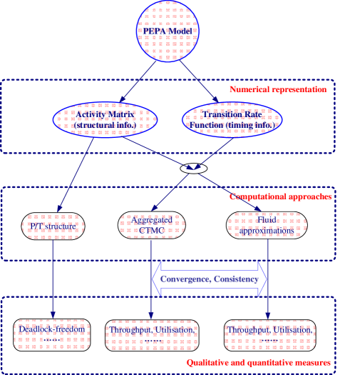
Figure 1: Three levels of PEPA modelling

The benefits of the schema embodies the three aspects of performance modelling, which are illustrated by Figure 1. At the first level, the proposed new schema numerically describes any given PEPA model and provides a platform to directly employ a variety of approaches to analyse the model. These approaches are shown at the second level. At this level, a fluid approximation method for the quantitative analysis of PEPA is established, as well as investigated, mainly with respect to its convergence and the consistency between this method and the underlying CTMC. In addition, a P/T structure-based approach is revealed, which can be utilised to qualitatively analyse the model. At the third level, both qualitative and quantitative performance measures can be derived from the model through those approaches. A stochastic simulation algorithm for the aggregated CTMC, which is based on the numerical representation schema, is proposed to obtain general performance metrics in this paper. As for the other two approaches, related investigation and analysis were given in [5] and [6] respectively, which will be briefly introduced in the next subsection.

1.2 Related work

Our work is motivated and stimulated by the pioneering work on the numerical vector form and activity matrix in [4], which was dedicated to the fluid approximation for PEPA. The P/T structure underlying each PEPA model, as stated in Theorem 1 in this paper, reveals tight connections between stochastic process algebras and stochastic Petri nets. Based on this structure and the theories developed for Petri nets, several powerful techniques for structural analysis of PEPA were presented in [5], including a structure-based deadlock-checking method which avoids the state space explosion problem. In [7], a new operational semantics was proposed to give a compact symbolic representation of PEPA models. This semantics extends the application scope of the fluid approximation of PEPA by incorporating all the operators of the language and removing earlier assumptions on the syntactical structure of the models amenable to this analysis. Moreover, the paper [6] shows how to derive the performance metrics such as action throughput and capacity utilisaition from the fluid approximation of a PEPA model.

1.3 Paper organisation

The remainder of this paper is structured as follows: Section 2 gives a brief introduction to the PEPA formulism; In Section 3, 4 and 5, we respectively present the three combinators of the numerical schema, i.e. the numerical vector form, labelled activity and activity matrix, as well as the transition rate function. Computational approaches for performance derivation that are developed on the basis of the schema are demonstrated in Section 6. We finally conclude the paper in Section 7.

2 Introduction to PEPA

PEPA (Performance Evaluation Process Algebra) [1], developed by Hillston in the 1990s, is a high-level model specification language for low-level stochastic models, and describes a system as an interaction of the components which engage in activities. In contrast to classical process algebras, activities are assumed to have a duration which is a random variable governed by an exponential distribution. Thus each activity in PEPA is a pair $(\alpha,r)$ where $\alpha$ is the action type and $r$ is the activity rate. The language has a small number of combinators, for which we provide a brief introduction below; the structured operational semantics can be found in [1]. The grammar is as follows:

$$S ::= (\alpha,r).S\mid S+S\mid C_{S}$$

$$P ::= P\raisebox{-4.30554pt}{$\;\stackrel{{\scriptstyle\mbox{\large$\rhd\!\!\!\lhd$}}}{{\scriptscriptstyle L}}\,$}P\mid P/L\mid C$$

where $S$ denotes a sequential component and $P$ denotes a model component which executes in parallel. $C$ stands for a constant which denotes either a sequential component or a model component as introduced by a definition. $C_{S}$ stands for constants which denote sequential components. The effect of this syntactic separation between these types of constants is to constrain legal PEPA components to be cooperations of sequential processes.

Prefix: The prefix component $(\alpha,r).S$ has a designated first activity $(\alpha,r)$, which has action type $\alpha$ and a duration which satisfies exponential distribution with parameter $r$, and subsequently behaves as $S$.

Choice: The component $S+T$ represents a system which may behave either as $S$ or as $T$. The activities of both $S$ and $T$ are enabled. Since each has an associated rate there is a race condition between them and the first to complete is selected. This gives rise to an implicit probabilistic choice between actions dependent of the relative values of their rates.

Hiding: Hiding provides type abstraction, but note that the duration of the activity is unaffected. In $P/L$ all activities whose action types are in $L$ appear as the “private” type $\tau$.

Cooperation:$P\raisebox{-4.30554pt}{$\;\stackrel{{\scriptstyle\mbox{\large$\rhd\!\!\!\lhd$}}}{{\scriptscriptstyle L}}\,$}Q$ denotes cooperation between $P$ and $Q$ over action types in the cooperation set $L$. The cooperands are forced to synchronise on action types in $L$ while they can proceed independently and concurrently with other enabled activities (individual activities). The rate of the synchronised or shared activity is determined by the slower cooperation (see [1] for details). We write $P\parallel Q$ as an abbreviation for $P\raisebox{-4.30554pt}{$\;\stackrel{{\scriptstyle\mbox{\large$\rhd\!\!\!\lhd$}}}{{\scriptscriptstyle L}}\,$}Q$ when $L=\emptyset$ and $P[N]$ is used to represent $N$ copies of $P$ in a parallel, i.e. $P[3]=P\parallel P\parallel P$.

Constant: The meaning of a constant is given by a defining equation such as $A\stackrel{{\scriptstyle\mbox{\em{\tiny def}}}}{{=}}P$. This allows infinite behaviour over finite states to be defined via mutually recursive definitions.

On the basis of the operational semantic rules (please refer to [1] for details), a PEPA model may be regarded as a labelled multi-transition system

$$\left(\mathcal{C},\mathcal{A}ct,\left\{\mathop{\longrightarrow}\limits^{(\alpha,r)}|(\alpha,r)\in\mathcal{A}ct\right\}\right)$$

where $\mathcal{C}$ is the set of components, $\mathcal{A}ct$ is the set of activities and the multi-relation $\mathop{\longrightarrow}\limits^{(\alpha,r)}$ is given by the rules. If a component $P$ behaves as $Q$ after it completes activity $(\alpha,r)$, then denote the transition as $P\mathop{\longrightarrow}\limits^{(\alpha,r)}Q$.

The memoryless property of the exponential distribution, which is satisfied by the durations of all activities, means that the stochastic process underlying the labelled transition system has the Markov property. Hence the underlying stochastic process is a CTMC. Note that in this representation the states of the system are the syntactic terms derived by the operational semantics. Once constructed the CTMC can be used to find steady-state or transient probability distributions from which quantitative performance can be derived.

3 Numerical Vector Form

The usual state representation in PEPA models is in terms of the syntactic forms of the model expression. When a large number of repeated components are involved in a system, the state space of the CTMC underling the model can be large. This is mainly because each copy of the same type of component is considered to be distinct, resulting in distinct Markovian states. The multiple states within the model that exhibit the same behaviour can be aggregated to reduce the size of the state space as shown by Gilmore et al. [8] using the technique based on a vector form. The CTMC is therefore constructed in terms of equivalence classes of syntactic terms. “At the heart of this technique is the use of a canonical state vector to capture the syntactic form of a model expression”, as indicated in [4]. Rather than the canonical representation style, an alternative numerical vector form was proposed by Hillston in [4] for capturing the state information of models with repeated components. In the numerical vector form, there is one entry for each local derivative of each type of component in the model. The entries in the vector are the number of components currently exhibiting this local derivative, no longer syntactic terms representing the local derivative of the sequential component. Following [4], hereafter the term local derivative refers to the local state of a single sequential component.

Definition 1.

(Numerical Vector Form[4]). For an arbitrary PEPA model $\mathcal{M}$ with $n$ component types ${C}_{i},i=1,2,\cdots,n$, each with $d_{i}$ distinct local derivatives, the numerical vector form of $\mathcal{M}$, $\mathbf{m}(\mathcal{M})$, is a vector with $d=\sum_{i=1}^{n}d_{i}$ entries. The entry $\mathbf{m}[{C}_{i_{j}}]$ records how many instances of the $j$th local derivative of component type ${C}_{i}$ are exhibited in the current state.

By adopting this model-aggregation technique, the number of the states of the system can be reduced to only increase (at most) polynomially with the number of instances of the components. According to Definition 1, $\mathbf{m}({C}_{i_{j}})\geq 0$ for each ${C}_{i_{j}}$. At any time, each sequential component stays in one and only one local derivative. So the sum of $\mathbf{m}({C}_{i})$, i.e. $\sum_{j=1}^{d_{i}}\mathbf{m}[{C}_{i_{j}}]$, specifies the population of ${C}_{i}$ in the system. Notice that $\mathbf{m}({C}_{i})$ satisfies

$$\left\{\begin{array}[]{c}\mathbf{m}[{C}_{i_{1}}],\mathbf{m}[{C}_{i_{2}}],\cdots,\mathbf{m}[{C}_{i_{d_{i}}}]\in\mathbb{Z}^{+},\\ \sum_{j=1}^{d}\mathbf{m}[{C}_{i_{j}}]=M_{i}.\end{array}\right.$$ (3.1)

Then according to the well-known combinatorial formula (Theorem 3.5.1 in [9]), there are $\left(\begin{array}[]{c}M_{i}+d_{i}-1\\ d_{i}-1\\ \end{array}\right)$ solutions, i.e. $\left(\begin{array}[]{c}M_{i}+d_{i}-1\\ d_{i}-1\\ \end{array}\right)$ states in terms of ${C}_{i}$ in the system. But the possible synchronisations in the PEPA model have not been taken into account in the restrictions (3.1) and thus the current restrictions may allow extra freedom for the solutions, so the given number $\left(\begin{array}[]{c}M_{i}+d_{i}-1\\ d_{i}-1\\ \end{array}\right)$ is an upper bound of the exact number of the states in terms of ${C}_{i}$. Notice that

$$\begin{split}\left(\begin{array}[]{c}M_{i}+d_{i}-1\\ d_{i}-1\\ \end{array}\right)=&\frac{(M_{i}+d_{i}-1)!}{(d_{i}-1)!M_{i}!}\\ \leq&\left(M_{i}+d_{i}-1\right)^{d_{i}-1}.\end{split}$$

Therefore, it is easy to verify the following

Proposition 1.

Consider a system comprising $n$ types of component, namely ${C}_{1},\mathcal{C}_{2},\cdots,{C}_{n}$, with $M_{i}$ copies of the component of type ${C}_{i}$ in the system, where ${C}_{i}$ has $d_{i}$ local derivatives, for $i=1,2,\cdots,n$. Then the size of the state space of the system is at most

$$\prod_{i=1}^{n}\left(\begin{array}[]{c}M_{i}+d_{i}-1\\ d_{i}-1\\ \end{array}\right)\leq\prod_{i=1}^{n}\left(M_{i}+d_{i}-1\right)^{d_{i}-1}.$$

The upper bound given in Proposition 1 guarantees that the size of the state space increases at most polynomially with the number of instances of the components. Consider the following PEPA model.

Model 1.

$$\begin{split}User_{1}\stackrel{{\scriptstyle\mbox{\em{\tiny def}}}}{{=}}&(task_{1},a).User_{2}\\ User_{2}\stackrel{{\scriptstyle\mbox{\em{\tiny def}}}}{{=}}&(task_{2},b).User_{1}\\ Sever_{1}\stackrel{{\scriptstyle\mbox{\em{\tiny def}}}}{{=}}&(task_{1},a).Sever_{2}\\ Sever_{2}\stackrel{{\scriptstyle\mbox{\em{\tiny def}}}}{{=}}&(reset,d).Sever_{1}\\ {User_{1}[M]}&\raisebox{-4.30554pt}{$\;\stackrel{{\scriptstyle\mbox{\large$\rhd\!\!\!\lhd$}}}{{\scriptscriptstyle\{task_{1}\}}}\,$}{Sever_{1}[N]}.\end{split}$$

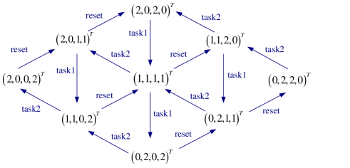
Figure 2: Transition between states (a revised version of the one in [4])

According to the semantics of PEPA originally defined in [1], the size of the state space of the CTMC underlying Model 1 is $2^{M+N}$, which increases exponentially with the numbers of the users and severs in the system. According to Definition 1, the system vector $\mathbf{m}$ has four entries representing the instances of components in the total four local derivatives, that is

$$\begin{split}\mathbf{m}=\left(\mathbf{m}[User_{1}],\mathbf{m}[User_{2}],\mathbf{m}[Sever_{1}],\mathbf{m}[Sever_{2}]\right)^{T}.\end{split}$$

Let $M=N=2$, then the system equation of Model 1 determines the starting state $(2,0,2,0)$. By enabling activities or transitions, all reachable system states can be manifested, see Figure 2. The size of the state space is nine. The upper bound of the size given by Proposition 1, $\left(\begin{array}[]{c}M+2-1\\ 2-1\\ \end{array}\right)\left(\begin{array}[]{c}N+2-1\\ 2-1\\ \end{array}\right)$ or $(M+1)\times(N+1)$, is nine, coinciding with the size of the state space. The bound given in Proposition 1 is sharp and can be hit in some situations.

4 Labelled Activity and Activity Matrix

In the PEPA language, the transition is embodied in the syntactical definition of activities, in the context of sequential components. Since the consideration is in terms of the whole system rather than sequential components, the transition between these system states should be defined and represented. This section presents a numerical representation for the transitions between system states and demonstrates how to derive this representation from a general PEPA model.

If a system vector changes into another vector after firing an activity, then the difference between these two vectors manifests the transition corresponding to this activity. Obviously, the difference is in numerical forms since all states are numerical vectors. Consider Model 1 and its transition diagram in Figure 2. Each activity in the model corresponds to a vector, called the transition vector. For example, $task_{1}$ corresponds to the transition vector $l^{task_{1}}=(-1,1,-1,1)^{T}$. That is, the derived state vector by firing $task_{1}$ from a state, can be represented by the sum of $l^{task_{1}}$ and the state enabling $task_{1}$. For instance, $(2,0,2,0)^{T}+l^{task_{1}}=(1,1,1,1)^{T}$ illustrates that $\mathbf{s}_{1}=(2,0,2,0)^{T}$ transitions into $\mathbf{s}_{2}=(1,1,1,1)^{T}$ after enabling $task_{1}$.

Table 1: Transition vectors form an activity matrix

	$l^{task_{1}}$	$l^{task_{2}}$	$l^{reset}$
$User_{1}$	$-1$	1	0
$User_{2}$	1	$-1$	0
$Sever_{1}$	$-1$	0	1
$Sever_{2}$	1	0	$-1$

Similarly, $task_{2}$ corresponds to $l^{task_{2}}=(1,-1,0,0)^{T}$ while $reset$ corresponds to $l^{reset}=(0,0,-1,1)$. The three transition vectors form a matrix, called the activity matrix, see Table 1. Each activity in the model is represented by a transition vector — a column of the activity matrix, and each column expresses an activity. So the activity matrix is essentially indicating both an injection and a surjection from syntactic to numerical representation of the transition between system states. The concept of the activity matrix for PEPA was first proposed by Hillston in [10, 4]. However, the original definition cannot fully reflect the representation mapping considered here. This is due to the fact of that the original definition is local-derivative-centric rather than transition centric. This results in some limitations for more general applications. For example, for some PEPA models (e.g. Model 2 in the following context), some columns of the originally defined matrix cannot be taken as transition vectors so that this definition cannot fully reflect the PEPA semantics in some circumstances. In the following, a modified definition of the activity matrix is given. The new definition is activity- or transition-centric, which brings the benefit that each transition is represented by a column of the matrix and vice versa.

Model 2.

$$\begin{split}P_{1}\stackrel{{\scriptstyle\mbox{\em{\tiny def}}}}{{=}}&(\alpha,r_{\alpha}^{\prime}).P_{2}+(\alpha,r_{\alpha}^{\prime\prime}).P_{3}\\ P_{2}\stackrel{{\scriptstyle\mbox{\em{\tiny def}}}}{{=}}&(\beta,r_{\beta}).P_{1}+(\beta,r_{\beta}^{\prime}).P_{3}\\ P_{3}\stackrel{{\scriptstyle\mbox{\em{\tiny def}}}}{{=}}&(\gamma,r_{\gamma}).P_{1}\\ Q_{1}\stackrel{{\scriptstyle\mbox{\em{\tiny def}}}}{{=}}&(\alpha,r_{\alpha}).Q_{2}\\ Q_{2}\stackrel{{\scriptstyle\mbox{\em{\tiny def}}}}{{=}}&(\gamma,r_{\gamma}^{\prime}).Q_{1}\\ {P_{1}[A]}&\raisebox{-4.30554pt}{$\;\stackrel{{\scriptstyle\mbox{\large$\rhd\!\!\!\lhd$}}}{{\scriptscriptstyle\{\alpha\}}}\,$}{Q_{1}[B]}.\end{split}$$

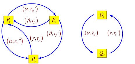
Figure 3: Transition diagram of Model 2

Table 2: Originally defined activity matrix of Model 2

	$\alpha$	$\beta$	$\gamma$
$P_{1}$	$-1$	$1$	1
$P_{2}$	$1$	$-1$	0
$P_{3}$	$1$	$1$	$-1$
$Q_{1}$	$-1$	0	$1$
$Q_{2}$	$1$	$0$	$-1$

Let us consider a PEPA model, i.e. the following Model 2, in which there are multiple choices after firing some activities. In this model, firing $\alpha$ in the component $P$ may lead to two possible local derivatives: $P_{2}$ and $P_{3}$, while firing $\beta$ may lead to $P_{1}$ and $P_{3}$. In addition, firing $\gamma$ may lead to $P_{1},Q_{1}$. However, only one derivative can be chosen after each firing of an activity, according to the semantics of PEPA. But the original definition of activity matrix cannot clearly reflect this point. See the activity matrix of Model 2 given in Table 2. Moreover, the individual activity $\gamma$ in this table, which can be enabled by both $P_{3}$ and $Q_{2}$, may be confused as a shared activity.

In order to better reflect the semantics of PEPA, we modify the definition of the activity matrix in this way: if there are $m$ possible outputs, namely $\{R_{1},R_{2},\cdots,R_{m}\}$, after firing either an individual or a shared activity $l$, then $l$ is “split” into $m$ labelled $l$s: $l^{w_{1}},l^{w_{2}},\cdots,l^{w_{m}}$. Here $\{w_{i}\}_{i=1}^{m}$ are $m$ distinct labels, corresponding to $\{R_{i}\}_{i=1}^{m}$ respectively. Each $l^{w_{i}}$ can only lead to a unique output $R_{i}$. Here there are no new activities created, since we just attach labels to the activity to distinguish the outputs of firing this activity. The modified activity matrix clearly reflects that only one, not two or more, result can be obtained from firing $l$. And thus, each $l^{w_{i}}$ can represent a transition vector.

For example, see the modified activity matrix of Model 2 in Table 3. In this activity matrix, the individual activity $\gamma$ has different “names” for different component types, so that it is not confused with a shared activity. Another activity $\beta$, is labelled as $\beta^{P_{2}\rightarrow P_{1}}$ and $\beta^{P_{2}\rightarrow P_{3}}$, to respectively reflect the corresponding two choices. In this table, the activity $\alpha$ is also split and attached with labels.

Table 3: Modified activity matrix of Model 2

	$\alpha^{(P_{1}\rightarrow P_{2},Q_{1}\rightarrow Q_{2})}$	$\alpha^{(P_{1}\rightarrow P_{3},Q_{1}\rightarrow Q_{2})}$	$\beta^{P_{2}\rightarrow P_{1}}$	$\beta^{P_{2}\rightarrow P_{3}}$	$\gamma^{P_{3}\rightarrow P_{1}}$	$\gamma^{Q_{2}\rightarrow Q_{1}}$
$P_{1}$	$-1$	$-1$	$1$	$0$	1	0
$P_{2}$	$1$	0	$-1$	$-1$	$0$	0
$P_{3}$	$0$	1	0	1	$-1$	0
$Q_{1}$	$-1$	$-1$	0	0	0	1
$Q_{2}$	$1$	1	0	0	$0$	$-1$

Before giving the modified definition of activity matrix for any general PEPA model, the pre and post sets for an activity are first defined. For convenience, throughout this paper any transition $U\stackrel{{\scriptstyle(l,r)}}{{\longrightarrow}}V$ defined in the PEPA models may be rewritten as $U\stackrel{{\scriptstyle(l,r_{l}^{U\rightarrow V})}}{{\longrightarrow}}V$, or just $U\stackrel{{\scriptstyle l}}{{\longrightarrow}}V$ if the rate is not being considered, where $U$ and $V$ are two local derivatives.

Definition 2.

(Pre and post local derivative)

1. If a local derivative $U$ can enable an activity $l$, that is $U\mathop{\longrightarrow}\limits^{l}\cdot$, then $U$ is called a pre local derivative of $l$. The set of all pre local derivatives of $l$ is denoted by $\mathrm{pre}(l)$, called the pre set of $l$.

2. If $V$ is a local derivative obtained by firing an activity $l$, i.e. $\cdot\mathop{\longrightarrow}\limits^{l}V$, then $V$ is called a post local derivative of $l$. The set of all post local derivatives is denoted by $\mathrm{post}(l)$, called the post set of $l$.

3. The set of all the local derivatives derived from $U$ by firing $l$, i.e.

   $$\mathrm{post}(U,l)=\{V\mid U\stackrel{{\scriptstyle l}}{{\longrightarrow}}V\},$$

   is called the post set of $l$ from $U$.

Obviously, if $l$ has only one pre local derivative, i.e. $\#\mathrm{pre}(l)=1$, then $l$ is an individual activity, like $\beta$ in Model 2, whereafter the notation $\#A$ is defined as the cardinality of the set $A$, i.e. the number of elements of $A$. But $l$ being individual does not imply $\#\mathrm{pre}(l)=1$, see $\gamma$ for instance. If $l$ is shared, then $\#\mathrm{pre}(l)>1$, for example, see $\#\mathrm{pre}(\alpha)=\#\{P_{1},Q_{1}\}=2$. For a shared activity $l$ with $\mathrm{pre}(l)=k$, there are $k$ local derivatives that can enable this activity, each of them belonging to a distinct component type. The obtained local derivatives are in the set $\mathrm{post}(\mathrm{pre}(l)[i],l)$, where $\mathrm{pre}(l)[i]$ is the $i$-th pre local derivative of $l$. But only one of them can be chosen after $l$ is fired from $\mathrm{pre}(l)[i]$. Since for the component type, namely $i$ or $\mathcal{C}_{i}$, there are $\#\mathrm{post}(\mathrm{pre}(l)[i],l)$ outputs, so the total number of the distinct transitions for the whole system is $\prod_{i=1}^{k}\#\mathrm{post}(\mathrm{pre}(l)[i],l).$ That is, there are $\prod_{i=1}^{k}\#\mathrm{post}(\mathrm{pre}(l)[i],l)$ possible results but only one of them can be chosen by the system after the shared activity $l$ is fired. In other words, to distinguish these possible transitions, we need $\prod_{i=1}^{k}\#\mathrm{post}(\mathrm{pre}(l)[i],l)$ different labels. Here are the readily accessible labels:

$$(\mathrm{pre}(l)[1]\rightarrow V_{1},\mathrm{pre}(l)[2]\rightarrow V_{2},\cdots,\mathrm{pre}(l)[k]\rightarrow V_{k}),$$

where $V_{i}\in\mathrm{post}(\mathrm{pre}(l)[i],l)$. Obviously, for each vector $(V_{1},V_{2},\cdots,V_{k})$ in $\mathrm{post}(\mathrm{pre}(l)[1],l)\times\mathrm{post}(\mathrm{pre}(l)[2],l)\times\cdots\times\mathrm{post}(\mathrm{pre}(l)[k],l),$ the labelled activity $l^{(\mathrm{pre}(l)[1]\rightarrow V_{1},\mathrm{pre}(l)[2]\rightarrow V_{2},\cdots,\mathrm{pre}(l)[k]\rightarrow V_{k})}$ represents a distinct transition. For example, $\alpha$ in Model 2 can be labelled as $\alpha^{(P_{1}\rightarrow P_{2},Q_{1}\rightarrow Q_{2})}$ and $\alpha^{(P_{1}\rightarrow P_{3},Q_{1}\rightarrow Q_{2})}$.

For an individual activity $l$, things are rather simple and easy: for $U\in\mathrm{pre}(l)$, $l$ can be labelled as $l^{U\rightarrow\mathrm{post}(U,l)[1]}$, $l^{U\rightarrow\mathrm{post}(U,l)[2]}$, $l^{U\rightarrow\mathrm{post}(U,l)[k_{U}]},$ where $k_{U}=\#\mathrm{post}(U,l)$. Varying $U\in\mathrm{pre}(l)$, there are $\sum_{U\in\mathrm{pre}(l)}\#\mathrm{post}(U,l)$ labels needed to distinguish the possible transitions. See $\beta^{P_{2}\rightarrow P_{1}},\beta^{P_{2}\rightarrow P_{3}},\gamma^{P_{3}\rightarrow P_{1}},\gamma^{Q_{2}\rightarrow Q_{1}}$ in Model 2 for instance. Now we give the formal definition.

Definition 3.

(Labelled Activity).

1. For any individual activity $l$, for each $U\in\mathrm{pre}(l),V\in\mathrm{post}(U,l)$, label $l$ as $l^{U\rightarrow V}$.

2. For a shared activity $l$, for each

   $$\begin{split}(V_{1},V_{2},\cdots,V_{k})\in\mathrm{post}(\mathrm{pre}(l)[1],l)\times\mathrm{post}(\mathrm{pre}(l)[2],l)\times\cdots\times\mathrm{post}(\mathrm{pre}(l)[k],l),\end{split}$$

   label $l$ as $l^{w}$, where

   $$\begin{split}w=(\mathrm{pre}(l)[1]\rightarrow V_{1},\mathrm{pre}(l)[2]\rightarrow V_{2},\cdots,\mathrm{pre}(l)[k]\rightarrow V_{k}).\end{split}$$

Each $l^{U\rightarrow V}$ or $l^{w}$ is called a labelled activity. The set of all labelled activities is denoted by $\mathcal{A}_{\mathrm{label}}$. For the above labelled activities $l^{U\rightarrow V}$ and $l^{w}$, their respective pre and post sets are defined as

$$\mathrm{pre}(l^{U\rightarrow V})=\{U\},\;\mathrm{post}(l^{U\rightarrow V})=\{V\},$$

$$\mathrm{pre}(l^{w})=\mathrm{pre}(l),\;\mathrm{post}(l^{w})=\{V_{1},V_{2},\cdots,V_{k}\}.$$

According to Definition 3, each $l^{U\rightarrow V}$ or $l^{w}$ can only lead to a unique output. No new activities are created, since labels are only attached to the activity to distinguish the results after this activity is fired.

The impact of labelled activities on local derivatives can be recorded in a matrix form, as defined below.

Definition 4.

(Activity Matrix). For a model with $N_{\mathcal{A}_{\mathrm{label}}}$ labelled activities and $N_{\mathcal{D}}$ distinct local derivatives, the activity matrix $\mathbf{C}$ is an $N_{\mathcal{D}}\times N_{\mathcal{A}_{\mathrm{label}}}$ matrix, and the entries are defined as follows

$$\mathbf{C}(U_{i},l_{j})=\left\{\begin{array}[]{cl}+1&\mbox{if $U_{i}\in\mathrm{post}(l_{j})$}\\ -1&\mbox{if $U_{i}\in\mathrm{pre}(l_{j})$}\\ 0&\mathrm{otherwise}\end{array}\right.$$

where $l_{j}$ is a labelled activity. The pre activity matrix $\mathbf{C^{pre}}$ and post activity matrix $\mathbf{C^{post}}$ are defined as

$$\mathbf{C^{Pre}}(P_{i},\alpha_{j})=\left\{\begin{array}[]{ll}+1&\mbox{if }\;\;P_{i}\in\mathrm{pre}(\alpha_{j})\\ 0&\mbox{otherwise}.\end{array}\right.,$$

$$\mathbf{C^{Post}}(P_{i},\alpha_{j})=\left\{\begin{array}[]{ll}+1&\mbox{if }\;\;P_{i}\in\mathrm{post}(\alpha_{j})\\ 0&\mbox{otherwise}.\end{array}\right.$$

The modified activity matrix captures all the structural information, including the information about choices and synchronisations, of a given PEPA model. From each row of the matrix, which corresponds to each local derivative, we can know which activities this local derivative can enable and after which activities are fired this local derivative can be derived. From the perspective of the columns, the number of “$-1$”s in a column tells whether the corresponding activity is synchronised or not. Only one “$-1$” means that this transition corresponds to an individual activity. The locations of “$-1$” and “$1$” indicate which local derivatives can enable the activity and what the derived local derivatives are, i.e. the pre and post local derivatives. In addition, the numbers of “$-1$”s and “$1$”s in each column are the same, because any transition in any component type corresponds to a unique pair of pre and post local derivatives. In fact, all this information is also stored in the labels of the activities. Therefore, with the transition rate functions defined in the next section to capture the timing information, a given PEPA model can be recovered from its activity matrix.

Moreover, the pre and post activity matrix indicate the local derivatives which can fire a labelled activity and the derived local derivative after firing a labelled activity respectively. The modified activity matrix equals the difference between the pre and post activity matrices, i.e. $\mathbf{C=C^{Post}-C^{Pre}}$. Hereafter the terminology of activity matrix refers to the one in Definition 4. This definition embodies the transition or operation rule of a given PEPA model, with the exception of timing information. For a given PEPA model, each transition of the system results from the firing of an activity. Each optional result after enabling this activity corresponds to a relevant labelled activity, that is, corresponds to a column of the activity matrix. Conversely, each column of the activity matrix corresponding to a labelled activity, represents an activity and the chosen derived result after this activity is fired. So each column corresponds to a system transition. Therefore, we have the following proposition, which specifies the correspondence between system transitions and the columns of the activity matrix.

Proposition 2.

Each column of the activity matrix corresponds to a system transition and each transition can be represented by a column of the activity matrix.

5 Transition Rate Function

The structural information of any general PEPA model is captured in the activity matrix, which is constituted by all transition vectors. However, the duration of each transition has not yet been specified. This section defines transition rate functions for transition vectors or labelled activities to capture the timing information of PEPA models.

5.1 Model 2 continued

Let us start from Model 2 again. As Table 3 shows, activity $\gamma$ in Model 2 is labelled as $\gamma^{P_{3}\rightarrow P_{1}}$ and $\gamma^{Q_{2}\rightarrow Q_{1}}$. For $\gamma^{P_{3}\rightarrow P_{1}}$, there are $\mathbf{x}[P_{3}]$ instances of the component type $P$ in the local derivative $P_{3}$ in state $\mathbf{x}$, each enabling the individual activity concurrently with the rate $r_{\gamma}$. So the rate of $\gamma^{P_{3}\rightarrow P_{1}}$ in state $\mathbf{x}$ is $f(\mathbf{x},\gamma^{P_{3}\rightarrow P_{1}})=r_{\gamma}\mathbf{x}[P_{3}]$. Similarly, the rate for $\gamma^{Q_{2}\rightarrow Q_{1}}$ in state $\mathbf{x}$ is $r_{\gamma^{\prime}}\mathbf{x}[Q_{2}]$. This is consistent with the definition of apparent rate in PEPA, which states that if there are $N$ replicated instances of a component enabling a transition $(l,r)$, the apparent rate of the activity will be $r\times N$.

In Model 2 activity $\beta$ is labelled as $\beta^{P_{2}\rightarrow P_{1}}$ and $\beta^{P_{2}\rightarrow P_{3}}$, to respectively reflect the corresponding two choices. According to the model definition, there is a flux of $r_{\beta}\mathbf{x}(P_{2})$ into $P_{1}$ from $P_{2}$ after firing $\beta$ in state $\mathbf{x}$. So the transition rate function is defined as $f(\mathbf{x},\beta^{P_{2}\rightarrow P_{1}})=r_{\beta}\mathbf{x}[P_{2}]$. Similarly, we can define $f(\mathbf{x},\beta^{P_{2}\rightarrow P_{3}})=r_{\beta}^{\prime}\mathbf{x}[P_{2}]$. These rate functions can be defined or interpreted in an alternative way. In state $\mathbf{x}$, there are $\mathbf{x}[P_{2}]$ instances that can fire $\beta$. So the apparent rate of $\beta$ is $(r_{\beta}+r_{\beta}^{\prime})\mathbf{x}[P_{2}]$. By the semantics of PEPA, the probabilities of choosing the outputs are $\frac{r_{\beta}}{r_{\beta}+r_{\beta}^{\prime}}$ and $\frac{r_{\beta}^{\prime}}{r_{\beta}+r_{\beta}^{\prime}}$ respectively. So the rate of the transition $\beta^{P_{2}\rightarrow P_{1}}$ is

$$f(\mathbf{x},\beta^{P_{2}\rightarrow P_{1}})=\frac{r_{\beta}}{r_{\beta}+r_{\beta}^{\prime}}(r_{\beta}+r_{\beta}^{\prime})\mathbf{x}[P_{2}]=r_{\beta}\mathbf{x}[P_{2}],$$ (5.2)

while the rate of the transition $\beta^{P_{2}\rightarrow P_{3}}$ is

$$f(\mathbf{x},\beta^{P_{2}\rightarrow P_{3}})=\frac{r_{\beta}^{\prime}}{r_{\beta}+r_{\beta}^{\prime}}(r_{\beta}+r_{\beta}^{\prime})\mathbf{x}[P_{2}]=r_{\beta}^{\prime}\mathbf{x}[P_{2}].$$ (5.3)

In Model 2, $\alpha$ is a shared activity with three local rates: $r_{\alpha},r_{\alpha}^{\prime}$ and $r_{\alpha}^{\prime\prime}$. The apparent rate of $\alpha$ in $P_{1}$ is $(r_{\alpha}^{\prime}+r_{\alpha}^{\prime\prime})\mathbf{x}[P_{1}]$, while in $Q_{1}$ it is $r_{\alpha}\mathbf{x}[Q_{1}]$. According to the PEPA semantics, the apparent rate of a synchronised activity is the minimum of the apparent rates of the cooperating components. So the apparent rate of $\alpha$ as a synchronisation activity is $\min\{(r_{\alpha}^{\prime}+r_{\alpha}^{\prime\prime})\mathbf{x}[P_{1}],r_{\alpha}\mathbf{x}[Q_{1}]\}$. After firing $\alpha$, $P_{1}$ becomes either $P_{2}$ or $P_{3}$, with the probabilities $\frac{r_{\alpha}^{\prime}}{r_{\alpha}^{\prime}+r_{\alpha}^{\prime\prime}}$ and $\frac{r_{\alpha}^{\prime\prime}}{r_{\alpha}^{\prime}+r_{\alpha}^{\prime\prime}}$ respectively. Simultaneously, $Q_{1}$ becomes $Q_{2}$ with the probability $1$. So the rate function of transition $(P_{1}\rightarrow P_{2},Q_{1}\rightarrow Q_{2})$, represented by $f(\mathbf{x},\alpha^{(P_{1}\rightarrow P_{2},Q_{1}\rightarrow Q_{2})})$, is

$$\begin{split}&f(\mathbf{x},\alpha^{(P_{1}\rightarrow P_{2},Q_{1}\rightarrow Q_{2})})\\ =&\frac{r_{\alpha}^{\prime}}{r_{\alpha}^{\prime}+r_{\alpha}^{\prime\prime}}\min\{(r_{\alpha}^{\prime}+r_{\alpha}^{\prime\prime})\mathbf{x}[P_{1}],r_{\alpha}\mathbf{x}[Q_{1}]\}.\end{split}$$ (5.4)

Similarly,

$$\begin{split}&f(\mathbf{x},\alpha^{(P_{1}\rightarrow P_{3},Q_{1}\rightarrow Q_{2})})\\ =&\frac{r_{\alpha}^{\prime\prime}}{r_{\alpha}^{\prime}+r_{\alpha}^{\prime\prime}}\min\{(r_{\alpha}^{\prime}+r_{\alpha}^{\prime\prime})\mathbf{x}[P_{1}],r_{\alpha}\mathbf{x}[Q_{1}]\}.\end{split}$$ (5.5)

The above discussion about the simple example should help the reader to understand the definition of transition rate function for general PEPA models, which is presented in the next subsection.

5.2 Definitions of transition rate function

In a PEPA model, as we have mentioned, we may rewrite any $U\stackrel{{\scriptstyle(l,r)}}{{\longrightarrow}}V$ as $U\stackrel{{\scriptstyle(l,r_{l}^{U\rightarrow V})}}{{\longrightarrow}}V$, where $r$ is denoted by $r_{l}^{U\rightarrow V}$. The transition rate functions of general PEPA models are defined below. We first give the definition of the apparent rate of an activity in a local derivative.

Definition 5.

(Apparent Rate of $l$ in $U$) Suppose $l$ is an activity of a PEPA model and $U$ is a local derivative enabling $l$ (i.e. $U\in\mathrm{pre}(l)$). Let $\mathrm{post}(U,l)$ be the set of all the local derivatives derived from $U$ by firing $l$, i.e. $\mathrm{post}(U,l)=\{V\mid U\stackrel{{\scriptstyle(l,r_{l}^{U\rightarrow V})}}{{\longrightarrow}}V\}.$ Let

$$r_{l}(U)=\sum_{V\in\mathrm{post}(U,l)}r_{l}^{U\rightarrow V}.$$ (5.6)

The apparent rate of $l$ in $U$ in state $\mathbf{x}$, denoted by $r_{l}(\mathbf{x},U)$, is defined as

$$r_{l}(\mathbf{x},U)=\mathbf{x}[U]r_{l}(U).$$ (5.7)

The above definition is used to define the following transition rate function.

Definition 6.

(Transition Rate Function) Suppose $l$ is an activity of a PEPA model and $\mathbf{x}$ denotes a state vector.

1. If $l$ is individual, then for each $U\stackrel{{\scriptstyle(l,r^{U\rightarrow V})}}{{\longrightarrow}}V$, the transition rate function of labelled activity $l^{U\rightarrow V}$ in state $\mathbf{x}$ is defined as

   $$f(\mathbf{x},l^{U\rightarrow V})=\mathbf{x}[U]r_{l}^{U\rightarrow V}.$$ (5.8)

2. If $l$ is synchronised, with $\mathrm{pre}(l)=\{U_{1},U_{2},\cdots,U_{k}\}$, then for each $(V_{1},V_{2},\cdots,V_{k})$ in $\mathrm{post}(U_{1},l)\times\mathrm{post}(U_{2},l)\times\cdots\times\mathrm{post}(U_{k},l),$ let $w=(U_{1}\rightarrow V_{1},U_{2}\rightarrow V_{2},\cdots,U_{k}\rightarrow V_{k})$. Then the transition rate function of labelled activity $l^{w}$ in state $\mathbf{x}$ is defined as

   $$f(\mathbf{x},l^{w})=\left(\prod_{i=1}^{k}\frac{r_{l}^{U_{i}\rightarrow V_{i}}}{r_{l}(U_{i})}\right)\min_{i\in\{1,\cdots,k\}}\{r_{l}(\mathbf{x},U_{i})\},$$

   where $r_{l}(\mathbf{x},U_{i})=\mathbf{x}[U_{i}]r_{l}(U_{i})$ is the apparent rate of $l$ in $U_{i}$ in state $\mathbf{x}$. So

   $$f(\mathbf{x},l^{w})=\left(\prod_{i=1}^{k}\frac{r_{l}^{U_{i}\rightarrow V_{i}}}{r_{l}(U_{i})}\right)\min_{i\in\{1,\cdots,k\}}\{\mathbf{x}[U_{i}]r_{l}(U_{i})\}.$$ (5.9)

Remark 1.

Definition 6 accommodates the passive or unspecified rate $\top$. If some $r^{U\rightarrow V}_{l}$ are $\top$, then the relevant calculation in the rate functions (5.8) and (5.9) can be made according to the inequalities and equations that define the comparison and manipulation of unspecified activity rates (see [1]). Moreover, we assume that $0\cdot\top=0$. So the terms such as “$\min\{A\top,rB\}$” are interpreted as [11]:

$$\min\{A\top,rB\}=\left\{\begin{array}[]{cc}rB,&A>0,\\ 0,&A=0.\end{array}\right.$$

The definition of the transition rate function is consistent with the semantics of PEPA:

Proposition 3.

The transition rate function in Definition 6 is consistent with the operational semantics of PEPA.

The proof is easy and omitted here. Since both the structural and timing information has been captured in the defined numerical representation schema, PEPA models can be therefore recovered from its representation schema. In addition, it is also easy to find that the transition rate function has the following homogenous property.

Proposition 4.

The transition rate function $f(\mathbf{x},l)$ satisfies that for any $H>0$, $Hf(\mathbf{x}/H,l)=f(\mathbf{x},l)$.

This property will identify the CTMCs underlying a PEPA model to be density dependent (see Theorem 4 in the next section).

5.3 Algorithm for deriving activity matrix and transition rate functions

This subsection presents an algorithm for automatically deriving the activity matrix and transition rate functions from any PEPA model, see Algorithm 1. The lines 3-12 of Algorithm 1 deal with individual activities while lines $13-32$ deal with shared activities. The calculation methods in this algorithm are essentially the embodiment of the definitions of labelled activity and apparent rate as well as transition rate function. So we do not give more introduction to this algorithm.

Algorithm 1 Derive activity matrix and transition rate functions from a general PEPA model

1:  $\mathcal{A}_{\mathrm{label}}=\emptyset$; $\mathcal{D}$ is the set of all local derivatives

2:  for all activity $l\in\mathcal{A}$ do

3:     if $l$ is an independent activity then

4:        for all local derivatives $U,V\in\mathcal{D}$ do

5:           if $U\stackrel{{\scriptstyle(l,r)}}{{\longrightarrow}}V$ then

6:              $\mathcal{A}_{\mathrm{label}}=\mathcal{A}_{\mathrm{label}}\cup\{l^{U\rightarrow V}\}$   // Label $l$ as $l^{U\rightarrow V}$

7:              // Form a corresponding column of the activity matrix and the rate function

8:              $M_{a}(d,l^{U\rightarrow V})=\left\{\begin{array}[]{ll}-1,&d=U\\ 1,&d=V\\ 0,&otherwise\end{array}\right.$

9:              $f(\mathbf{x},l^{U\rightarrow V})=r\mathbf{x}[U]$

10:           end if

11:        end for

12:     end if

13:     if $l$ is a synchronised activity then

14:        $\mathrm{pre}(l)=\emptyset,\mathrm{post}(U,l)=\emptyset,\;\forall U\in\mathcal{D}$

15:        for all local derivatives $U,V\in\mathcal{D}$ do

16:           if $U\stackrel{{\scriptstyle(l,r)}}{{\longrightarrow}}V$ then

17:              $\mathrm{pre}(l)=\mathrm{pre}(l)\cup\{U\}$

18:              $\mathrm{post}(U,l)=\mathrm{post}(U,l)\cup\{V\}$

19:              $r_{l}^{U\rightarrow V}=r$

20:           end if

21:        end for

22:        Denote $\mathrm{pre}(l)=\{\mathrm{pre}(l)[1],\mathrm{pre}(l)[2],\cdots,\mathrm{pre}(l)[k]\}$, where $k=\#\mathrm{pre}(l)$

23:        for $i=1\dots k$ do

24:           $r_{l}(\mathrm{pre}(l)[i])=\sum\limits_{V\in\mathrm{post}({\mathrm{pre}(l)[i]},l)}r_{l}^{\mathrm{pre}(l)[i]\rightarrow V}$

25:        end for

26:        $K(l)=\mathrm{post}({\mathrm{pre}(l)[1],l})\times\mathrm{post}({\mathrm{pre}(l)[2]},l)\times\cdots\times\mathrm{post}({\mathrm{pre}(l)[k]},l)$

27:        for all $(V_{1},V_{2},\cdots,V_{k})\in K(l)$ do

28:           $w=(\mathrm{pre}(l)[1]\rightarrow V_{1},\mathrm{pre}(l)[2]\rightarrow V_{2},\cdots,\mathrm{pre}(l)[k]\rightarrow V_{k})$

29:           $\mathcal{A}_{\mathrm{label}}=\mathcal{A}_{\mathrm{label}}\cup\{l^{w}\}$   // Label $l$ as $l^{w}$

30:           // Form a column of $M_{a}$ and the rate function corresponding to $l^{w}$

$$M_{a}(d,l^{w})=\left\{\begin{array}[]{ll}-1,&d\in\mathrm{pre}(l)\\ 1,&d\in\{V_{1},V_{2},\cdots,V_{k}\}\\ 0,&otherwise\end{array}\right.$$

$$\begin{split}&f(\mathbf{x},l^{w})=\left(\prod_{i=1}^{k}\frac{r_{l}^{\mathrm{pre}(l)[i]\rightarrow V_{i}}}{r_{l}(\mathrm{pre}(l)[i])}\right)\min_{i\in\{1,\cdots,k\}}\{r_{l}(\mathrm{pre}(l)[i])\mathbf{x}[\mathrm{pre}(l)[i]]\}\end{split}$$

31:        end for

32:     end if

33:  end for

34:  Output $\mathcal{A}_{\mathrm{label}}$; $M_{a}$; $f(\mathbf{x},l)\;(\forall l\in\mathcal{A}_{\mathrm{label}})$.

6 Computational approaches for PEPA

As a model being represented numerically, efficient techniques such as stochastic simulation and fluid approximation can be can be directly utilised to analyse the model. This section briefly introduces these approaches as well as technical foundations for employing them in the context of PEPA.

6.1 Place/Transition structure in PEPA models

Whilst the focus of stochastic process algebras has understandably been primarily quantitative analysis, qualitative analysis can also provide valuable insight into the behaviour of a system. In contrast, in Petri net modelling there are well-established techniques of structural analysis [12, 13, 14]. This subsection shows how the new representation schema helps to manifest the P/T structure underlying PEPA models, and makes it possible to readily adapt structural analysis techniques for Petri nets to PEPA. First, the relevant definitions are given below.

Definition 7.

(P/T net, Marking, P/T system, [14])

1. A Place/Transition net (P/T net) is a structure $\mathcal{N}=(P,T,\mathbf{Pre,Post})$ where: $P$ and $T$ are the sets of places and transitions respectively; $\mathbf{Pre}$ and $\mathbf{Post}$ are the $|P|\times|T|$ sized, natural valued, incidence matrices.

2. A marking is a vector $\mathbf{m}:P\rightarrow\mathbb{N}$ that assigns to each place of a P/T net a nonnegative integer (number of tokens).

3. A P/T system is a pair $\mathcal{S}=\langle\mathcal{N},\mathbf{m_{0}}\rangle$: a net $\mathcal{N}$ with an initial marking $\mathbf{m_{0}}$.

By Definition 7, it is easy and direct to verify

Theorem 1.

There is a P/T system underlying any PEPA model, that is $\langle\mathcal{N},\mathbf{m_{0}}\rangle$, where $\mathbf{m_{0}}$ is the starting state; $\mathcal{N}=\left(\mathcal{D},\mathcal{A}_{\small\mbox{label}},\mathbf{C^{\mbox{Pre}},C^{\mbox{Post}}}\right)$ is P/T net: where $\mathcal{D}$ is the set of local derivatives, $\mathcal{A}_{\small\mbox{label}}$ is the labelled activity set; $\mathbf{C^{\mbox{Pre}}}$ and $\mathbf{C^{\mbox{Post}}}$ are the pre and post activity matrices respectively. Moreover, each state $\mathbf{m}$ of the PEPA model is a marking.

Based on the P/T structure underlying PEPA models and the theories developed for P/T nets, several powerful techniques and approaches for structural analysis of PEPA were established in [5]. For instance, the authors gave a method of deriving and storing the state space which avoids the problems associated with populations of components, and an approach to find invariants which can be used to qualitatively reason about systems. Moreover, a structure-based deadlock-checking algorithm was proposed, which can avoid the state space explosion problem.

6.2 Stochastic simulation of PEPA models

By solving the global balance equations associated with the infinitesimal generator of the CTMC underlying a PEPA model, the steady-state probability distribution can be obtained, from which performance measures can be derived. According to the original definition of the PEPA language in which each instance of the same component type is considered distinctly, the size of the state space of this original CTMC may increase exponentially with the number of components. By adopting the numerical vector form to represent the system state which results in the aggregated CTMC, the size of the state space can thus be significantly reduced, as Proposition 1 shows, together with the computational complexity of deriving the performance by solving the corresponding global balance equations since, the dimension of the infinitesimal generator matrix is the square of the size of the state space.

Unless otherwise stated, hereafter the CTMC underlying a PEPA model refers to the aggregated CTMC, and the state of a model or a system is considered in the sense of aggregation. If the size of the state space is too large, it is not feasible to calculate the steady-state distribution and thus to get a performance measure $R$, which is usually expressed as $R=\sum_{\mathbf{s}\in S}\rho(\mathbf{s})\mathbf{\pi}(\mathbf{s})$ where $\rho$ and $\mathbf{\pi}$ defined on the state space $S$ are the reward function and the steady-state probability distribution respectively. An alternative widely-used way to obtained performance is stochastic simulation.

As discussed previously, a transition between states, namely from $\mathbf{x}$ to $\mathbf{x}+l$, is represented by a transition vector $l$ corresponding to the labelled activity $l$ (for convenience, hereafter each pair of transition vectors and corresponding labelled activities shares the same notation). The rate of the transition $l$ in state $\mathbf{x}$ is specified by the transition rate function $f(\mathbf{x},l)$. That is, $\mathbf{x}\mathop{\longrightarrow}\limits^{(l,f(\mathbf{x},l))}\mathbf{x}+l.$ Given a starting state $\mathbf{x}_{0}$, the transition chain corresponding to a firing sequence $l_{0},l_{1},\cdots,l,\cdots$ is

$$\begin{split}&\mathbf{x}_{0}\mathop{\longrightarrow}\limits^{(l_{0},f(\mathbf{x}_{0},l_{0}))}\mathbf{x}_{0}+l_{0}\mathop{\longrightarrow}\limits^{(l_{1},f(\mathbf{x}_{0}+l_{0},l_{1}))}(\mathbf{x}_{0}+l_{0})+l_{1}\mathop{\longrightarrow}\limits^{\cdots}\\ &\cdots\mathop{\longrightarrow}\limits^{\cdots}\mathbf{x}\mathop{\longrightarrow}\limits^{(l,f(\mathbf{x},l))}\mathbf{x}+l\mathop{\longrightarrow}\limits^{\cdots}\cdots.\end{split}$$

The above sequence can be considered as one path or realisation of a simulation of the aggregated CTMC, if the enabled activity at each state is chosen stochastically, i.e. is chosen through the approach of sampling. After a long time, the steady-state of the system is assumed to be achieved. Hence the average performance $R=\sum_{\mathbf{s}\in S}\rho(\mathbf{s})\mathbf{\pi}(\mathbf{s})$ can be calculated.

As one benefit of our numerical representation schema, it provides a good platform for directly and conveniently simulating the CTMC for PEPA, see Algorithm 2. In Algorithm 2, the states of a PEPA model are represented as numerical vector forms, and the rates between those states are specified by the transition rate functions which only depend on the transition type (i.e. labelled activity) and the current state. In this algorithm, the generated time $\tau$ in each iteration can be regarded as having been drawn from an exponential distribution with the mean $\displaystyle\frac{1}{f(\mathbf{x})}$ (see Example 2.3 in [15], page 38). That is, Line $9$ in Algorithm 2 is in fact expressing: “generate $\tau$ from an exponential distribution with the mean $\displaystyle\frac{1}{f(\mathbf{x})}$”. Line $10$ determines which transition will be chosen, and consequently determines the next state that the system will transition into. Therefore, this algorithm is essentially to simulate the CTMC underlying a PEPA model.

Algorithm 2 Simulation algorithm for deriving general performance measures from PEPA model

1:  //Initialisation

2:  starting state $\mathbf{x}$; labelled activity set $\mathcal{A}_{\mathrm{label}}=\{l_{1},l_{2},\cdots,l_{m}\}$; activity matrix; transition rate function $f$

3:  reward function $\rho$; $\mathrm{PerMeasure}=0$

4:  while stop condition not satisfied do

5:     //Sampling

6:     compute the transition rate function $\displaystyle{f(\mathbf{x},l_{j})}$, $j=1,2,\cdots,m$

7:     $f(\mathbf{x})=\sum_{j=1}^{m}f(\mathbf{x},l_{j})$

8:     generate uniform random numbers $r_{1},r_{2}$ on $[0,1]$

9:     compute $\tau=-(1/f(\mathbf{x}))\ln r_{1}$

10:     find $\mu$ such that $\sum_{j=1}^{\mu-1}f(\mathbf{x},l_{j})\leq r_{2}f(\mathbf{x})<\sum_{j=1}^{\mu}f(\mathbf{x},l_{j})$

11:     //Updating

12:     $\mathrm{PerMeasure}=\mathrm{PerMeasure}+\rho(\mathbf{x})\times\tau$  // Accumulate performance measure

13:     $t=t+\tau$  //Accumulate time

14:     $\mathbf{x}=\mathbf{x}+l_{\mu}$  // Update state vector of system

15:  end while

16:  Output performance: $\frac{\mathrm{PerMeasure}}{t}$

The choices for stopping the algorithm include a given large time, or the absolute or relative error of two continued iterations being small enough (since the output performance converges as time goes to infinity as the following Theorem 3 states). Now we prove the convergence of the performance calculated using the algorithm. We need the following theorem.

Theorem 2.

(Theorem 3.8.1, [16]) If $X(t)$ is an irreducible and positive recurrent CTMC with the state space $S$ and the unique invariant distribution $\mathbf{\pi}$, then

$$\mathrm{Pr}\left(\frac{1}{t}\int_{0}^{t}1_{\{X_{z}=\mathbf{s}\}}\mathrm{d}z\rightarrow\mathbf{\pi}(\mathbf{s})\mbox{ as }t\rightarrow\mathchar 561\relax\right)=1.$$ (6.10)

Moreover, for any bounded function $\rho:S\rightarrow\mathbb{R}$, we have

$$\mathrm{Pr}\left(\frac{1}{t}\int_{0}^{t}\rho(X_{z})\mathrm{d}z\rightarrow E[\rho(X)]\mbox{ as }t\rightarrow\mathchar 561\relax\right)=1.$$ (6.11)

where $E[\rho(X)]=\sum_{\mathbf{s}\in S}\rho(\mathbf{s})\mathbf{\pi}(\mathbf{s})$.

Here is our conclusion (we assume the CTMCs underlying PEPA models to be irreducible and positive recurrent):

Theorem 3.

The performance measure calculated according to Algorithm 2 converges as time goes to infinity, that is, $\lim_{t\rightarrow\mathchar 561\relax}\frac{\mathrm{PerMeasure}}{t}=E[\rho(X)]$.

Proof.

Assume that $n-1$ iterations have been finished and the time has accumulated to $t_{n-1}$. Suppose the current one is the $n$-th iteration and $\tau$ is the generated time in this iteration. After the $n$-th iteration is finished, the accumulated time will be updated to $t_{n}=t_{n-1}+\tau$. During the $\tau$ time interval, the simulated CTMC stays in the state $\mathbf{x}$, that is, $X_{z}=\mathbf{x},z\in[t_{n-1},t_{n})$. So,

$$\begin{split}&\rho(\mathbf{x})\times\tau\\ =&\rho(\mathbf{x})\int_{t_{n-1}}^{t_{n}}\mathrm{d}z=\int_{t_{n-1}}^{t_{n}}\rho(\mathbf{x})\mathrm{d}z=\int_{t_{n-1}}^{t_{n}}\rho(X_{z})\mathrm{d}z.\end{split}$$

Therefore, after this $n$-th iteration, $\mathrm{PerMeasure}$ will be accumulated to $=\int_{0}^{t_{n}}\rho(X_{z})\mathrm{d}z$ and

$$\frac{\mathrm{PerMeasure}}{t_{n}}=\frac{1}{t_{n}}\int_{0}^{t_{n}}\rho(X_{z})\mathrm{d}z.$$

According to Theorem 2, $\displaystyle\frac{1}{t_{n}}\int_{0}^{t_{n}}\rho(X_{z})\mathrm{d}z$ tends to $E[\rho(X)]$ as $t_{n}$ tends to infinity. So the performance obtained through Algorithm 2 converges to $E[\rho(X)]$ as the simulation time goes to infinity. ∎

Performance metrics, such as activity throughput of an activity and capacity utilisation of a local derivative that are discussed in [6], can be derived through this algorithm by choosing appropriate reward functions.

6.3 Fluid approximation of PEPA models

The weakness of the simulation method is its high computational cost, which makes it not suitable for real-time performance monitoring or prediction. Recently, a novel approach to get performance measures from PEPA models has been proposed in [4] and subsequently expanded in [7] and [17], making a continuous state space approximation as a set of ordinary differential equations (ODEs). In this section, we present a mapping semantics for this approaches, which is based on the numerical representation schema. In addition, a theoretical justification of this approach, mainly in terms of its consistency with the CTMCs, will be discussed.

In our representation schema, the transition rate $f(\mathbf{x},l)$ reflects the intensity of the transition from state $\mathbf{x}$ to state $\mathbf{x}+l$. The state space is inherently discrete with the entries within the numerical vector form always being non-negative integers and always being incremented or decremented in steps of one. As pointed out in [4], when the numbers of components are large these steps are relatively small and we can approximate the behaviour by considering the movement between states to be continuous, rather than occurring in discontinuous jumps. In fact, let us consider the evolution of the numerical state vector. Denote the state at time $t$ by $\mathbf{x}(t)$. In a short time $\Delta t$, the change to the vector $\mathbf{x}(t)$ will be

$$\begin{split}\mathbf{x}(\cdot,t+\Delta t)-\mathbf{x}(\cdot,t)=\Delta t\sum_{l\in\mathcal{A}_{\mathrm{label}}}lf(\mathbf{x}(\cdot,t),l).\end{split}$$

Dividing by $\Delta t$ and taking the limit, $\Delta t\rightarrow 0$, we obtain a set of ODEs:

$$\frac{\mathrm{d}\mathbf{x}}{\mathrm{d}t}=\sum_{l\in\mathcal{A}_{\mathrm{label}}}lf(\mathbf{x},l).$$ (6.12)

Once the activity matrix and the transition rate functions are generated, the ODEs are immediately available. All of them can be obtained automatically by Algorithm 1.

For an arbitrary CTMC, the evolution of probabilities distributed on each state can be described using linear ODEs (see [18], page 52). For example, for the aggregated CTMC underlying a PEPA model, the corresponding differential equations are

$$\frac{\mathrm{d}\mathbf{\pi}}{\mathrm{d}t}=Q^{T}\mathbf{\pi},$$ (6.13)

where each entry of $\mathbf{\pi}(t)$ represents the probability of the system being in each state at time $t$, and $Q$ is an infinitesimal generator matrix corresponding to the CTMC. Clearly, the dimension of the coefficient matrix $Q$ is the square of the size of the state space, which increases with the number of components.

The scale of (6.13), i.e. the number of the ODEs, depends on the size of the state space, so it suffers from the state sapce explosion problem. In contrast, the ODEs (6.12) reflect the evolution of the population of the components in each local derivative, so the scale is only determined by the number of local derivatives and is unaffected by the size of the state space. Therefore, it avoids the explosion problem. But the price paid is that the ODEs (6.12) are generally nonlinear due to synchronisations, whereas (6.13) is linear.

This paper emphasises the consistency between the fluid approximation and the aggregated CTMC. Obviously, the CTMC depends on the starting state of the given PEPA model. By altering the population of components presented in the model, which can be done by varying the initial states, we may get a sequence of aggregated CTMCs. Moreover, the homogenous property that the transition rate function satisfies, indicated in Proposition 4, identifies the aggregated CTMC to be density dependent.

Definition 8.

([19]). A family of CTMCs $\{X_{n}\}_{n}$ is called density dependent if and only if there exists a continuous function $f(\mathbf{x},l),\;\mathbf{x}\in\mathbb{R}^{d},\;l\in\mathbb{Z}^{d}$, such that the infinitesimal generators of $X_{n}$ are given by:

$$q^{(n)}_{\mathbf{x},\mathbf{x}+l}=nf(\mathbf{x}/n,l),\quad l\neq 0,$$

where $q^{(n)}_{\mathbf{x},\mathbf{x}+l}$ denotes an entry of the infinitesimal generator of $X_{n}$, $\mathbf{x}$ a numerical state vector and $l$ a transition vector.

This allows us to immediately conclude the following conclusion:

Theorem 4.

([17, 7]) Let $\{X_{n}\}$ be a sequence of aggregated CTMCs generated from a given PEPA model (by scaling the initial state), then $\{X_{n}\}$ is density dependent.

Since both ODEs and density dependent CTMCs can be derived from the same PEPA model through the same activity matrix and transition rate functions, it is natural to believe some kind of consistency between them. In fact, according to Kurtz’s theorem [20], the complete solution of some ODEs can be the limit of a sequence of Markov chains. Such consistency in the context of PEPA has been previously illustrated for a particular PEPA model in [21], and subsequently generalised to general models in [7] and [17]. The result presented below is extracted from [17], in which the convergence is in the sense of almost surely rather than probabilistically as in [21] and [7].

Theorem 5.

([17]) Let $\mathbf{x}(t)$ be the solution of the ODEs (6.12) derived from a given PEPA model with initial condition $\mathbf{x}_{0}$, and let $\{X_{n}(t)\}$ be the density dependent CTMCs with $X_{n}(0)=n\mathbf{x}_{0}$. Then for any $t>0$,

$$\lim_{n\rightarrow\mathchar 561\relax}\sup_{u\leq t}\left\|X_{n}(u)/n-\mathbf{x}(u)\right\|=0\quad\quad a.s.$$ (6.14)

This theorem justifies the fluid approximation by manifesting the consistency between this approach and the corresponding CTMCs for a general PEPA model. Furthermore, if there is no synchronisation contained in the model then the derived ODEs (6.12) becomes linear, and (6.13) and (6.12) coincide except for a constant factor. Moreover, the fundamental results on the fluid approximation of PEPA models such as the existence, uniqueness, boundedness and nonnegativeness of the ODEs’ solution, as well as the solution’s asymptotic behaviour, have been obtained. In particular, the convergence of the ODEs’ solution as time tends to infinity, has been proved under a condition, which is revealed to relate to some famous constants of Markov chains such as the spectral gap and the Log-Sobolev constant. For more details about these stories, please refer to [22]. As for performance derivation via this approach, please see [6].

7 Conclusions

In this paper we have demonstrated a schema, which bridges the syntactic and numerical representation, as well as the local definition and global analysis for a PEPA model. Computational approaches and associated algorithms developed based on the schema have been presented, which can help to relieve the state space explosion problem for large scale models. For other stochastic process algebras, similar numerical representation schema can be established and expected to benefit relevant performance modelling.

References

- [1] J. Hillston, A Compositional Approach to Performance Modelling (PhD Thesis). Cambridge University Press, 1996.
- [2] N. Götz, U. Herzog, and M. Rettelbach, “TIPP– a language for timed processes and performance evaluation,” tech. rep., Tech. Rep.4/92, IMMD7, University of Erlangen-Nörnberg, Germany, Nov. 1992.
- [3] M. Bernardo and R. Gorrieri, “A tutorial on EMPA: A theory of concurrent processes with nondeterminism, priorities, probabilities and time,” Theoretical Computer Science, vol. 202, pp. 1–54, 1998.
- [4] J. Hillston, “Fluid flow approximation of PEPA models,” in International Conference on the Quantitative Evaluation of Systems (QEST’05), IEEE Computer Society, 2005.
- [5] J. Ding and J. Hillston, “Structural analysis for stochastic process algebra models (invited paper),” in Proceedings of Thirteenth International Conference on Algebraic Methodology and Software Technology (AMAST2010), (Manoir St-Castin Québec,Canada), 2010.
- [6] M. Tribastone, J. Ding, S. Gilmore, and J. Hillston, “Fluid rewards for a stochastic process algebra,” 2010. Submitted to IEEE Transactions on Software Engineering.
- [7] M. Tribastone, S. Gilmore, and J. Hillston, “Scalable differential analysis of process algebra models,” 2010. To appear in IEEE Transactions on Software Engineering.
- [8] S. Gilmore, J. Hillston, and M. Ribaudo, “An efficient algorithm for aggregating PEPA models,” IEEE Trans. Softw. Eng., vol. 27, no. 5, pp. 449–464, 2001.
- [9] R. A. Brualdi, Introductory Combinatorics. Prentice Hall, third ed., 1998.
- [10] M. Calder, S. Gilmore, and J. Hillston, “Automatically deriving ODEs from process algebra models of signalling pathways,” in Proc. of 3rd International Workshop on Computational Methods in Systems Biology (CMSB) (G. Plotkin, ed.), (Edinburgh), pp. 204–215, April 2005.
- [11] J. T. Bradley, S. T. Gilmore, and J. Hillston, “Analysing distributed internet worm attacks using continuous state-space approximation of process algebra models,” Journal of Computer and System Sciences, vol. 74, pp. 1013–1032, September 2008.
- [12] K. Lautenbach, “Linear algebraic techniques for place/transition nets,” in Petri Nets: Central Models and Their Properties, vol. 254 of Lecture Notes in Computer Science, pp. 142–167, Springer Berlin / Heidelberg, 1987.
- [13] M. Silva, E. Teruel, and J. M. Colom, “Linear algebraic and linear programming techniques for the analyisis of place/transition net systems,” in Lecture Notes in Computer Science, vol. 1491, Springer-Verlag, 1996.
- [14] J. M. Colom, E. Teruel, and M. Silva, “Logical properties of P/T system and their analysis.” MATCH Summer School (Spain), Septemper 1998.
- [15] S. Asmussen and P. W. Glynn, Stochastic Simulation: Algorithms and Analysis, vol. 57 of Stochastic Modelling and Applied Probability. Springer, 2007.
- [16] J. Norris, Markov Chains. Cambridge Series in Statistical and Probabilistic Mathematics, Cambridge University Press, July 1998.
- [17] J. Ding, Structural and Fluid Analysis of Large Scale PEPA models — with Applications to Content Adaptation Systems. PhD thesis, The Univeristy of Edinburgh, 2010. http://www.dcs.ed.ac.uk/pepa/jie-ding-thesis.pdf.
- [18] G. Bolch, S. Greiner, H. d. Meer, and K. S. Trivedi, Queueing Networks and Markov Chains: Modelling and Performance Evaluation with Computer Science Application. John Wiley & Sons, INC., 1998.
- [19] T. G. Kurtz, “Solutions of ordinary differential equations as limits of pure jump Markov processes,” Journal of Applied Probability, vol. 7, no. 1, pp. 49–58, 1970.
- [20] S. N. Ethier and T. G. Kurtz, Markov Processes: Characterization and Convergence. John Wiley & Sons, Inc., 1986.
- [21] N. Geisweiller, J. Hillston, and M. Stenico, “Relating continuous and discrete PEPA models of signalling pathways,” Theoretical Computer Science, vol. 404, pp. 97–111, Sep. 2008.
- [22] J. Ding and J. Hillston, “Fundamental results of fluid approximations of PEPA models.” http://arxiv.org/abs/1008.4754, Aug. 2010.