The Least Spanning Area of a Knot
and the Optimal Bounding Chain Problem

Abstract

Two fundamental objects in knot theory are the minimal genus surface and the least area surface bounded by a knot in a 3-dimensional manifold. When the knot is embedded in a general 3-manifold, the problems of finding these surfaces were shown to be $\mathbf{NP}$-complete and $\mathbf{NP}$-hard respectively. However, there is evidence that the special case when the ambient manifold is $\mathbb{R}^{3}$, or more generally when the second homology is trivial, should be considerably more tractable. Indeed, we show here that a natural discrete version of the least area surface can be found in polynomial time.

The precise setting is that the knot is a 1-dimensional subcomplex of a triangulation of the ambient 3-manifold. The main tool we use is a linear programming formulation of the Optimal Bounding Chain Problem (OBCP), where one is required to find the smallest norm chain with a given boundary. While the decision variant of OBCP is $\mathbf{NP}$-complete in general, we give conditions under which it can be solved in polynomial time. We then show that the least area surface can be constructed from the optimal bounding chain using a standard desingularization argument from 3-dimensional topology.

We also prove that the related Optimal Homologous Chain Problem is $\mathbf{NP}$-complete for homology with integer coefficients, complementing the corresponding result of Chen and Freedman for mod 2 homology.

1 Introduction

A knot $K$ is a simple closed loop in an ambient 3-dimensional manifold $Y$. Provided $K$ is null-homologous, which is always the case if $Y=\mathbb{R}^{3}$, there is an embedded orientable surface $S$ in $Y$ whose boundary is $K$ (equivalently $S$ is a compact smooth orientable surface in $Y$ without self-intersections and with boundary $K$). A fundamental property of $K$ is the minimal genus of such an $S$, which is denoted $g(K)$ (we take $g(K)=\infty$ if there are no such surfaces). In the 1960s, Haken used normal surface theory to give an algorithm for computing $g(K)$, opening the door to a whole subfield of low-dimensional topology and leading to the discovery of algorithms for determining a wide range of topological properties of 3-manifolds MatveevAlgorithmsBook . However, algorithms based on normal surface theory are quite slow in practice Burton2010b ; Burton2010a ; Burton2010c , and there are very few results that have been verified via such normal surface computations DunfieldGaroufalidis2010 ; BurtonRubinsteinTillmann2010 . Moreover, in some cases the underlying problems have been shown to be fundamentally difficult. In their foundational work, Agol, Hass, and Thurston showed that the following decision problem is $\mathbf{NP}$–complete AgolHassThurston :

1.1 Knot Genus.

Given an integer $g_{0}$ and a knot $K$ embedded in the 1-skeleton of a triangulation of a closed 3-manifold $Y$, is $g(K)\leq g_{0}$?

While Knot Genus is $\mathbf{NP}$–complete, when $Y$ is orientable and the second Betti number $b_{2}(Y)=\mathrm{rank}\,\big{(}H_{2}(Y;\mathbb{Z})\big{)}$ is $0$, for instance $Y=S^{3}$, then this problem likely simplifies. While their project is not yet complete, Agol, Hass, and Thurston have developed a very promising approach to showing that when $b_{2}(Y)=0$ there is a certificate for the complementary problem $g(K)\geq g_{0}$ which can be verified in polynomial time. This would mean that this special case of Knot Genus is also in co-NP, raising the possibility of a polynomial-time algorithm when $b_{2}(Y)=0$. However, currently there are no known algorithms which exploit the fact that $b_{2}(Y)=0$. Despite this, our long-term goal is

1.2 Conjecture.

For orientable $Y$ with $b_{2}(Y)=0$ the Knot Genus problem is in P.

Here, we study the related problem of finding the least area surface bounded by a knot. This problem has its origin in classical differential geometry, as we now sketch starting with the case where the ambient manifold $Y$ is $\mathbb{R}^{3}$. For a smooth knot $K$ in $\mathbb{R}^{3}$ there is always a smooth embedded orientable surface $S\subset\mathbb{R}^{3}$ with $\partial S=K$. By deep theorems in Geometric Measure Theory, there always exists such a surface $S_{0}$ of least area MorganGMTBook . A least area surface $S_{0}$ is necessarily minimal in that it has mean curvature 0 everywhere, like the surface of a soap-bubble. It is typically impossible to find the least area surface analytically, and the first paper on numerical methods for approximating $S_{0}$ appeared in 1927 Douglas1927 . An algorithm to deal with arbitrary $K$ was first given by Sullivan SullivanThesis in 1990; see also Parks1986 ; Parks1992 ; ParksPitts1997 ; PinkallPolthier1993 ; Polthier2005 for alternate approaches and numerical experiments.

Of course, one can consider this question for null-homologous knots in an arbitrary Riemannian 3-manifold $Y$, and one has the same existence theorems for least area surfaces when $Y$ is closed. Agol, Hass, and Thurston considered a certain discrete version of this problem, and showed that the question of whether $K$ bounds a surface of area $\leq A_{0}$ is $\mathbf{NP}$-hard AgolHassThurston . Because they put no restriction on the surface involved, it is not clear if their question is in $\mathbf{NP}$. Here, we consider another discretization, the Least Spanning Area Problem of Section 5, which is a little more combinatorial and will thus turn out to be $\mathbf{NP}$-complete (Theorem 5.2). For this problem, we show

1.3 Theorem.

For orientable $Y$ with $b_{2}(Y)=0$ the Least Spanning Area Problem is in P.

In Section 6, we discuss how the ideas behind Theorem 1.3 might be used to attack Conjecture 1.2, as these two questions have a very similar flavor.

One of two key tools behind Theorem 1.3 is the following type of combinatorial optimization problem. For a finite simplicial complex $X$, fix an $\ell^{1}$-norm on the simplicial chains $C_{*}(X;\mathbb{Z})$ by assigning each simplex an arbitrary nonnegative weight. (For example, every simplex could have weight 1, or if $X$ is a geometric mesh in $\mathbb{R}^{3}$ one could take each weight to be the length/area/volume of the simplex itself.) For a chain $a\in C_{n}(X;\mathbb{Z})$ the Optimal Homologous Chain Problem (OHCP) is to find a chain $c\in C_{n}(X;\mathbb{Z})$ homologous to $a$ with $\lVert c\rVert_{1}$ minimal. As there are many choices for $c$, this might seem like a hard problem. Indeed, consider the decision problem variant, OHCP-D: given $X$, $a$, and $L\in\mathbb{N}$ is there a $c$ homologous to $a$ with $\lVert c\rVert_{1}\leq L$? We show:

1.4 Theorem.

The OHCP-D with integer coefficients is NP-complete.

Chen and Freedman established the same result when one uses homology with $\mathbb{F}_{2}$-coefficients ChFr2010aalt . However, with the addition of a simple condition on $X$ (which often holds in geometric applications), Dey, Hirani, and Krishnamoorthy DeHiKr2010 have used linear programming to solve the OHCP for $\mathbb{Z}$ coefficients in polynomial time, and this will be a key tool here.

We also need to consider the related Optimal Bounding Chain Problem (OBCP): given $b\in C_{n-1}(X;\mathbb{Z})$, find the $c\in C_{n}(X;\mathbb{Z})$ where $\partial_{n}c=b$ and $\lVert c\rVert_{1}$ is minimal. (Of course, this is only interesting when $[b]$ is $0$ in $H_{n-1}(X;\mathbb{Z})$ as otherwise no such $c$ exists.) If $H_{n}(X)=0$ then the OBCP is equivalent to a related instance of the OHCP (Theorem 2.4). Thus one can often use the method of DeHiKr2010 to solve such problems quickly (Cor. 2.5). Conversely, we describe how a key construction in AgolHassThurston shows that the decision problem variant of OBCP is $\mathbf{NP}$-complete in general (Theorem 4.2), and we then modify the construction to prove Theorem 1.4.

To prove Theorem 1.3, we reduce the Least Area Surface problem to the OBCP via a standard desingularization method from 3-dimensional topology that turns an arbitrary 2-cycle into an embedded surface that is homologous to it. This surface can be built constructively, and we outline in Section 6 how this gives an approach to Conjecture 1.2. As a preview to this material, we give an simple application of the OBCP in Section 3 to the toy problem of finding the shortest path between opposite sides of a triangulated square.

2 Optimal chain problems

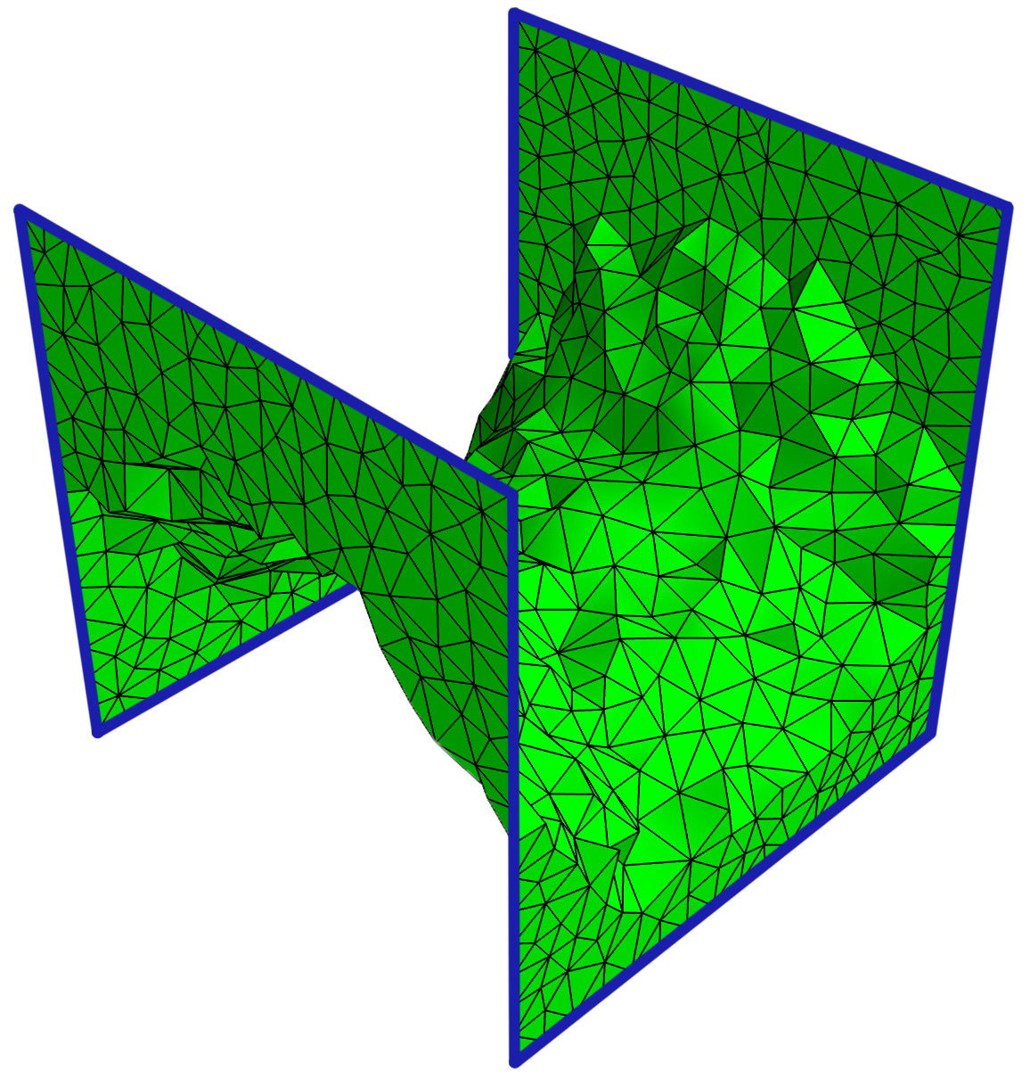
Figure 2.1: The surface shown is the solution to the OBCP for the 1-cycle $b$ shown in dark blue. Here $X$ is a cube triangulated with 19,201 tetrahedra, 39,758 triangles, 24,256 edges and 3,700 vertices, and the 1-cycle $b$ is a Hamiltonian cycle of the cube corners. The surface approximates Scherk’s minimal surface.

For the rest of this paper, all homology will be over $\mathbb{Z}$, and so we drop the coefficients from the notation. As in the introduction, we consider a finite simplicial complex $X$ with an $\ell^{1}$-norm on $C_{*}(X)$, and recall the Optimal Homologous Chain Problem (OHCP): given $a\in C_{n}(X)$, minimize $\lVert c\rVert_{1}$ over all $c=a+\partial_{n+1}x$ with $x\in C_{n+1}(X)$. (Here $a$ need not be a cycle.) The framework of DeHiKr2010 is that minimizing $\lVert c\rVert_{1}$ can be reformulated as minimizing some linear functional over the lattice points in a convex region defined by linear inequalities, i.e. an integer linear programming problem. While integer linear programming is $\mathbf{NP}$-complete, when the matrix for the boundary map $\partial_{n+1}\colon\thinspace C_{n+1}(X)\to C_{n}(X)$ is totally unimodular (meaning every subdeterminant is in $\{-1,0,1\}$), the OHCP reduces to an ordinary linear programming (LP) problem, and those can be solved in polynomial time. This LP problem is the integer program with the integrality constraints dropped, i.e., it is the LP relaxation of the integer linear program. Total unimodularity implies that the constraint polyhedron is integral VeDa1968 , and thus so is the solution to the linear program.

There is a simple criterion for when $\partial_{n+1}$ is totally unimodular. Recall that a pure subcomplex of $X$ of dimension $k$ is a union of $k$-simplices of $X$ including all their subsimplices. We say that $X$ is relatively torsion-free in dimension $n$ if $H_{n}(L,L_{0})$ is torsion-free for all pure subcomplexes $L_{0}\subset L$ of dimensions $n$ and $n+1$ respectively. Examples include any orientable manifold of dimension $n+1$, or any simplicial complex that embeds in $\mathbb{R}^{n+1}$. It turns out that $\partial_{n+1}$ is totally unimodular if and only if $X$ is relatively torsion-free in dimension $n$ and so:

2.2 Theorem (DeHiKr2010 ).

If $X$ is relatively torsion-free in dimension $n$ then the OHCP for $a\in C_{n}(X)$ can be solved in polynomial time.

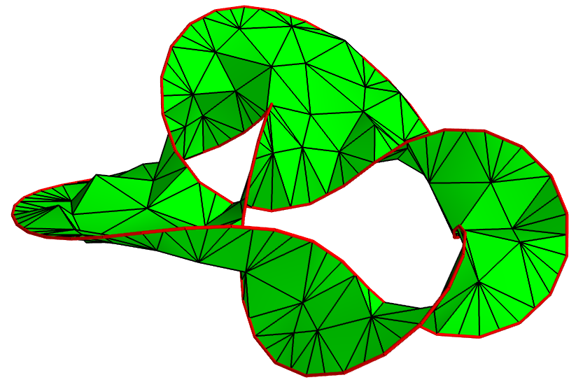
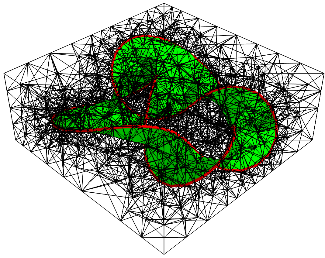
Figure 2.3: At top is the solution (green) to the OBCP for the 1-cycle that is given by the knot $5_{2}$ (red). The knot is a subcomplex of the 1-skeleton of a tetrahedral mesh of a cuboid shown in the lower picture.

Turning now to the Optimal Bounding Chain Problem (OBCP), assume that instead we are given a lower dimensional chain $b\in C_{n-1}(X)$ and we seek the minimum norm $c\in C_{n}(X)$ whose boundary is this $b$. (Of course, if $[b]\in H_{n-1}(X)$ is nonzero this question is moot.) Some examples are shown in Figures 2.1 and 2.3. For certain $X$ we can relate these two problems:

2.4 Theorem.

Suppose $a\in C_{n}(X)$ is such that $b=\operatorname{\partial}_{n}a$. If $H_{n}(X)=0$ then the OHCP (for that $a$) is identical to the OBCP (for that $b$). Hence they have the same optimal solutions.

Proof.

In both problems, we seek a $c\in C_{n}(X)$ of minimal $\ell^{1}$-norm, so the claim is that the constraints on $c$ are actually the same in either case. Since $H_{n}(X)=0$, having $b=\partial_{n}c$ is equivalent to $c=a+\partial_{n+1}x$ as if we have the former then $\partial_{n}(c-a)=b-b=0$ and thus there is an $x$ with $\partial_{n+1}x=c-a$. ∎

2.5 Corollary.

Suppose $H_{n}(X)=0$ and $X$ is relatively torsion-free in dimension $n$. Then the OBCP for $b\in C_{n-1}(X)$ can be solved in polynomial time.

Proof.

Set up the OBCP for $b$ as an integer LP, and then quickly solve its LP relaxation. If $b$ is not a boundary, then the feasible set is empty and we’re done. Otherwise, we claim the solution is actually integral. By Theorem 2.4 this LP is identical to one for the OHCP for some (uncomputed) $a\in C_{n}(X)$. From our discussion of the proof of Theorem 2.2, we know the latter LP has an integral solution as needed. ∎

2.6 Remark.

Consider a Möbius strip embedded in $\mathbb{R}^{3}$. Enclose it in a cube and triangulate the cube with tetrahedra such that the strip is part of the 2-skeleton of the complex. Let $X$ be the cube triangulation and $b$ the 1-cycle carried by the topological boundary of the Möbius strip. Here $\operatorname{\partial}_{3}$ is totally unimodular, which guarantees that $X$ is relatively torsion-free in dimension 2, as required by Cor. 2.5. When we solve the OBCP problem as a relaxed LP, the constraints are $\partial_{2}c=b$. The constraint matrix $\operatorname{\partial}_{2}$ is not totally unimodular DeHiKr2010 . Nevertheless, Cor. 2.5 guarantees that the minimizer $c$ will be integral. This does not contradict the result about equivalence of total unimodularity and integrality. That result says that total unimodularity is equivalent to the integrality of the constraint polyhedron for all right-hand sides in the polyhedral constraint equations. Whereas in Cor. 2.5 we are saying that the solution is integral if the right-hand side $b$ is in the image of $\partial_{2}$ which certainly doesn’t include all 1-chains in $X$.

2.7 Previous work on OBCP

The OBCP in the trivial homology case as above has appeared in Sullivan’s thesis SullivanThesis , and in the work of Grady Grady2010alt and that of Gortler and his coworkers KiGo2004 . When in addition $X$ is an $(n+1)$-manifold, Sullivan gave a polynomial time algorithm for the OBCP based on network flow. This idea also appears in KiGo2004 and related work. The basic idea in KiGo2004 is that the cycle $b$ of dimension $n-1$ is on the boundary of the domain with trivial $H_{n}(X)$. One introduces a source and a sink and connects them to the centers of the top dimensional simplices on the boundary. These edges are given infinite capacity. The dual graph of the codimension-1 skeleton then forms the rest of the edges in the network and these edges have capacities equal to the volumes of the primal codimension-1 faces. Then by the maxflow-mincut theorem one obtains a maxflow and hence an optimal chain. It is an interesting question whether such network flow methods can also be used to prove the more general Cor. 2.5 which only requires that $X$ be relatively torsion-free in dimension $n$.

3 A relative version of the OBCP and a toy problem

In geometric applications, one often cares not about the specifics of the cycle $b\in C_{n-1}(X)$ but only its homology class in some subcomplex $A\subset X$. Before stating the problem in this context, we recall the basics of relative homology. The relative chain groups are $C_{n}(X,A)=C_{n}(X)/C_{n}(A)$ which we also identify with the submodule $C_{n}(X\setminus A)$ of $C_{n}(X)$. The boundary maps for $C_{*}(X,A)$ are induced from those of $C_{*}(X)$. When $C_{n}(X,A)$ is viewed as $C_{n}(X\setminus A)$, a relative cycle $c$ is simply one where the support of $\partial_{n}c$ is contained in $A$. Thus a relative cycle gives rise to an element $[\partial_{n}c]$ in $H_{n-1}(A)$ since $\partial_{n-1}\circ\partial_{n}=0$. (This map from relative cycles to $H_{n-1}(A)$) is just the connecting homomorphism in the long exact sequence of the pair Munkres1984 .) We can now pose:

3.1 Relative OBCP.

Let $A$ be a subcomplex of $X$, and $\beta\in H_{n-1}(A)$. Find a relative cycle $c\in C_{n}(X,A)$ so that $[\partial_{n}c]=\beta$ and $\lVert c\rVert_{1}$ is minimal.

3.2 Theorem.

Suppose $H_{n}(X)=0$ and $X$ is relatively torsion-free in dimension $n$. Then the relative OBCP for $\beta\in H_{n-1}(A)$ can be solved in polynomial time.

Proof.

Suppose $\beta\in H_{n-1}(A)$ is specified by a cycle $b\in C_{n-1}(A)$. First, we can quickly find a chain $c\in C_{n}(X)$ with $\partial_{n}c=b$ (or determine that none exists) either by solving a linear system over $\mathbb{Z}$ Dixon1982 or by solving this instance of the ordinary OBCP via Corollary 2.5.

Suppose $c^{\prime}\in C_{n}(X)$ is any other chain with $\partial_{n}c^{\prime}=b^{\prime}$ where $b^{\prime}\in C_{n-1}(A)$ also represents $\beta$. Since $H_{n}(X)=0$, it follows that $[c]=[c^{\prime}]$ in the relative homology group $H_{n}(X,A)$. Thus, solving the relative OBCP for $\beta$ is the same as solving the OHCP for $C_{n}(X,A)$. By the discussion in Section 2, it is enough to show the relative boundary map $\partial_{n+1}\colon\thinspace C_{n+1}(X,A)\to C_{n}(X,A)$ is totally unimodular. This is the case since its matrix is obtained by deleting certain rows and columns from that of the original $\partial_{n+1}\colon\thinspace C_{n+1}(X)\to C_{n}(X)$. ∎

3.3 Toy problem

We next give a quick application to a simple problem that nonetheless has all the features of our proof of Theorem 1.3 in Section 5. Let $X$ be a simplicial complex homeomorphic to a square, and let $L$ and $R$ be subcomplexes corresponding to a pair of opposite sides. We will show that Theorem 3.2 allows us to solve the following problem in polynomial time:

3.4 Problem.

Find the shortest embedded simplicial path in the 1-skeleton of $X$ joining $L$ to $R$.

See Figure 3.5 for an example.

Figure 3.5: A path which uses the fewest possible number of edges to join the two vertical sides.

Of course, this problem can be solved very efficiently by a variety of algorithms. We give it primarily to introduce the idea of desingularization which is needed for Theorem 1.3. Let $A=L\cup R$. Then $H_{0}(A)=\mathbb{Z}\oplus\mathbb{Z}$ is generated by $[v_{L}]$ and $[v_{R}]$ for any vertices $v_{L}$ and $v_{R}$ in $L$ and $R$ respectively. Now $\beta=[v_{R}]-[v_{L}]$ is $0$ in $H_{0}(X)$ and so consider relative cycles $c\in C_{1}(X,A)$ with $[\partial_{1}c]=\beta$. Any embedded simplicial path from $L$ to $R$ gives such a $c$, but of course not every such $c$ comes from a path (e.g. the coefficient on some edge could be greater than $1$). However, we will show that if $\lVert c\rVert_{1}$ is minimal then it does come from an embedded path. This is necessarily the path of minimal length, and hence we will have reduced Problem 3.4 to the relative OBCP for $\beta$. Since $H_{1}(X)=0$, Theorem 3.2 applies to let us quickly find $c$, and hence answer Problem 3.4.

Figure 3.6: At left is part of a 1-cycle $c$ on a portion of a triangulated surface. At right is a desingularization of it. The resulting path need not be unique, but such a path will always exist. See Section 5.3 for the higher dimensional desingularization.

Suppose $c$ is any relative cycle in $C_{1}(X,A)$. The following desingularization procedure gives a collection of oriented embedded loops and arcs which give the same class in $H_{1}(X,A)$. Along an edge $e$ of $X$ where $c$ has coefficient $w$, we put $\lvert w\rvert$ strands parallel to $e$ oriented appropriately. Then near each vertex $v$ of $X\setminus A$ we connect up the strands without introducing any crossings as shown in Figure 3.6. Because $\partial_{1}c=0$ at $v$, we can do this respecting the orientations of the strands. That is, at the vertices, there is an outgoing strand for every incoming one. Thus we can build a set of loops and arcs homologous to $c$.

Now suppose $c$ minimizes $\lVert c\rVert_{1}$ among the relative cycles with $[\partial_{1}c]=\beta$. In the desingularization of $c$ there must be at least one arc from $L$ to $R$, as for instance arcs joining $L$ to itself give $0$ in $H_{0}(A)$. Slightly moving this arc, we push it back onto the 1-skeleton $X^{1}$ of $X$ to give another relative cycle $c^{\prime}\in C_{1}(X,A)$ with $[\partial_{1}c^{\prime}]=\beta$. The coefficient of $c^{\prime}$ on any edge is at most that of $c$, and so by minimality of $\lVert c\rVert_{1}$ we must have $c=c^{\prime}$. Thus $c$ corresponds to an oriented path in $X^{1}$. Moreover, this path must visit any given vertex at most once, since otherwise a segment of the path forms a closed loop which could be eliminated to reduce $\lVert c\rVert_{1}$. Thus $c$ gives an embedded path from $L$ to $R$, as claimed.

4 NP-completeness of the OBCP and the OHCP

In this section, we explain how the work of Agol, Hass, and Thurston AgolHassThurston shows that the decision problem variant of OBCP is $\mathbf{NP}$-complete, and then use this to prove that the OHCP-D is also $\mathbf{NP}$-complete. Precisely, consider the following decision problem:

4.1 OBCP-D.

Given a simplicial complex $X$, a chain $b\in C_{n-1}(X)$, and an $L\in\mathbb{N}$, is there a chain $c\in C_{n}(X)$ with $\partial_{n}c=b$ and $\lVert c\rVert_{1}\leq L$?

Here the complexity is in terms of the number of simplices in $X$ plus the logs of $\lVert b\rVert_{1}$ and $L$. We will show:

4.2 Theorem.

The OBCP-D is NP-complete.

The proof of this is essentially contained in AgolHassThurston , and indeed they use some clever tricks to reduce more geometric problems like Knot Genus to the more combinatorial OBCP-D, though they do not use the latter language explicitly. Despite this, we include a complete proof of Theorem 4.2 as we need to modify the construction to prove Theorem 1.4. As a bonus, the simpler context of the OBCP-D makes the idea of AgolHassThurston easier to digest for those not familiar with 3-manifold theory.

One of two key ideas in AgolHassThurston is the following construction, which relates the OBCP-D to 1-in-3 SAT, which is $\mathbf{NP}$-complete GareyJohnson1979 ; Schaefer1978 . Recall that in 1-in-3 SAT, we are given boolean variables $U=\{u_{1},\ldots,u_{n}\}$ and clauses $C=\{c_{1},\ldots,c_{m}\}$, where each clause contains three literals ($u_{i}$ or its negation ${{\mkern 3.5mu\overline{\mkern-3.5muu\mkern-1.5mu}\mkern 1.5mu}}_{i}$) joined by $\vee$. The question is whether there is a truth assignment for $U$ so that each clause has exactly one true literal. We now build a 2-complex $X$ associated to an instance of 1-in-3 SAT by gluing together several planar surfaces, that is, 2-spheres with (open) discs removed. Throughout this discussion, consult Figure 4.3 for an example.

Figure 4.3: The complex $X$ associated to $(u_{2}\vee{{\mkern 3.5mu\overline{\mkern-3.5muu\mkern-1.5mu}\mkern 1.5mu}}_{2}\vee{{\mkern 3.5mu\overline{\mkern-3.5muu\mkern-1.5mu}\mkern 1.5mu}}_{1})\wedge(u_{2}\vee u_{3}\vee{{\mkern 3.5mu\overline{\mkern-3.5muu\mkern-1.5mu}\mkern 1.5mu}}_{3})$.

The base surface $F_{0}$ has $n+m+1$ boundary components, one labeled by the symbol $K$ and the others by the elements of $U\cup C$. There is also a surface $F_{u}$ for each variable $u\in U$, which has one boundary component labeled by $u$, and the others labeled by $c\in C$ for each time $u$ (but not ${{\mkern 3.5mu\overline{\mkern-3.5muu\mkern-1.5mu}\mkern 1.5mu}}$) occurs in $c$. For the negation of each variable $u$ there is a surface $F_{{{\mkern 3.5mu\overline{\mkern-3.5muu\mkern-1.5mu}\mkern 1.5mu}}}$ with one boundary component labeled $u$ and the others labeled by the appearances of ${{\mkern 3.5mu\overline{\mkern-3.5muu\mkern-1.5mu}\mkern 1.5mu}}$ in the clauses. When only $u$ or ${{\mkern 3.5mu\overline{\mkern-3.5muu\mkern-1.5mu}\mkern 1.5mu}}$ appears in the clauses, then one of the surfaces is simply a disc.

We triangulate each surface $F$ so that every boundary component consists of three 1-simplices and the number of 2-simplices in $F$ is $5\lvert\partial F\rvert-4$, where $\lvert\partial F\rvert$ denotes the number of connected components of $\partial F$. For each $F$, we fix consistent orientations of its 2-simplices to create a relative cycle which generates $H_{2}(F,\partial F)\cong\mathbb{Z}$; we denote the corresponding chain in $C_{2}(F)$ by $[F]$. Now we build $X$ by gluing together all boundary components with the same labels, in such a way that the gluings between $F_{0}$ (where every label appears) and any $F_{u}$ or $F_{{\mkern 3.5mu\overline{\mkern-3.5muu\mkern-1.5mu}\mkern 1.5mu}}$ is orientation reversing; in particular, $\partial_{2}([F_{0}]+[F_{u}])$ is $0$ along the circle labeled $u$. We let $b$ be the 1-cycle that corresponds to the boundary component of $F_{0}$ that is labeled $K$, oriented so that it appears in $\partial_{2}[F_{0}]$. The key lemma is:

4.4 Lemma.

The 1-in-3 SAT instance $(U,C)$ has a solution if and only if there exists $d\in C_{2}(X)$ with $b=\partial_{2}d$ and $\lVert d\rVert_{1}\leq 1+6n+10m$.

Proof.

To start, observe that if we denote the set of literals by $V=U\cup{\big{\{}{{{\mkern 3.5mu\overline{\mkern-3.5muu\mkern-1.5mu}\mkern 1.5mu}}}\ \big{|}\ {u\in U}\big{\}}}$ then any solution $d$ to $b=\partial_{2}d$ necessarily has the form

$$d=[F_{0}]+\sum_{v\in V}k_{v}[F_{v}]\quad\mbox{for some $k_{v}$ in $\mathbb{Z}$}$$

and the boundary of any such chain is supported on the labeled circles. Since each 2-simplex lies in exactly one surface, the chains in the sum above have disjoint supports, and an easy calculation gives

$$\lVert d\rVert_{1}=1+5n+5m+\lVert k_{V}\rVert_{1}+5\sum_{v\in V}\lvert k_{v}\rvert m_{v}$$

where $k_{V}$ is the vector $(k_{v})$ and $m_{v}$ is the number of times $v$ appears in the clauses $C$. Using $x_{c},y_{c},z_{c}$ to denote the literals that appear in a clause $c$, we can rewrite this as:

$$\lVert d\rVert_{1}=1+5n+5m+\lVert k_{V}\rVert_{1}+5\sum_{c\in C}\left(\lvert k_{x_{c}}\rvert+\lvert k_{y_{c}}\rvert+\lvert k_{z_{c}}\rvert\right)$$ (4.5)

To start the proof proper, first suppose we have a solution to the 1-in-3 SAT instance, and let $d$ be the chain where $k_{v}$ is $1$ or $0$ depending on whether $v$ is true or false. For each variable $u$, one of $k_{u}$ and $k_{{\mkern 3.5mu\overline{\mkern-3.5muu\mkern-1.5mu}\mkern 1.5mu}}$ is $1$ and the other $0$; hence taking into account the contribution from $F_{0}$, we see that $\partial d$ is $0$ along the circle labeled $u$. Now for a circle labeled by a clause $c$, as exactly one literal in $c$ is true we again see that $\partial d$ is $0$ along this circle. Hence $\partial d=b$, and (4.5) gives that $\lVert d\rVert_{1}=1+6n+10m$.

Conversely, let $d$ be a chain with $\partial d=b$ and $\lVert d\rVert_{1}\leq 1+6n+10m$. As $\partial d$ is 0 along the circle labeled by $u$, it follows that at least one of $k_{u}$ and $k_{{\mkern 3.5mu\overline{\mkern-3.5muu\mkern-1.5mu}\mkern 1.5mu}}$ is nonzero, and hence $\lVert k_{V}\rVert\geq n$. Similarly, for each clause $c$ at least one of $k_{x_{c}},k_{y_{c}},k_{z_{c}}$ must be nonzero to ensure $d$ has no boundary along the circle labeled $c$. Hence from (4.5) and the bound on $\lVert d\rVert_{1}$ it follows that $\lVert k_{V}\rVert=n$ and each summand in the right-hand sum is $1$. Thus exactly one of $k_{u}$ and $k_{{\mkern 3.5mu\overline{\mkern-3.5muu\mkern-1.5mu}\mkern 1.5mu}}$ is 1 and the other 0, and each clause has exactly one $F_{v}$ surface coming into it having nonzero weight. Therefore $d$ corresponds to the needed solution to the 1-in-3 SAT instance. ∎

It is now easy to prove Theorem 4.2 and then adapt this construction to show Theorem 1.4.

Proof of Theorem 4.2.

The OBCP-D is in $\mathbf{NP}$ as we can use the cycle $c$ itself as the certificate. One just has to check that $\partial c=b$, and this matrix vector multiplication is polynomial in the number of simplices in $X$. Conversely, the OBCP-D is $\mathbf{NP}$-hard since given an instance of 1-in-3 SAT, by Lemma 4.4 there is an associated 2-complex $X$ (made from $O(n+m)$ simplices) and a 1-cycle $b$ so that a solution to the 1-in-3 SAT problem is equivalent to finding $c$ with $\partial c=b$ and $\lVert c\rVert_{1}\leq 1+6n+10m$. ∎

Proof of Theorem 1.4.

Let $CX$ be the cone on $X$, which is a 3-dimensional simplicial complex. Let $Y$ be the 3-complex obtained from $CX$ by attaching a 2-simplex $\sigma$ to the boundary component of $F_{0}\subset X\subset CX$ labeled $K$. For convenience, we use an $\ell^{1}$-norm on $C_{2}(Y)$ so that each 2-simplex in $X^{\prime}=X\cup\sigma$ has weight 1, but the rest each have weight $10+6n+10m$. As $CX$ is contractible, the space $Y$ is homotopy equivalent to $S^{2}$, and hence $H_{2}(Y)=\mathbb{Z}$. Let $a\in C_{2}(Y)$ generate $H_{2}(Y)$ and have weight $+1$ on $\sigma$, where $\sigma$ is oriented compatibly with $F_{0}$. We claim that our instance of 1-in-3 SAT has a solution if and only if $a$ is homologous to a cycle of weight at most $2+6n+10m$. Such a cycle would have to be confined to $X^{\prime}$, and thus have the form $\sigma+d$ where $d$ is as in the proof of Lemma 4.4, proving our claim and hence the theorem. ∎

5 Least area surfaces bounded by a knot

Recall from Section 1 that a basic question about a smooth knot $K$ in a closed Riemannian 3-manifold $Y$ is the minimal area of an embedded surface $S$ with boundary $K$. Agol, Hass, and Thurston AgolHassThurston considered the following discrete version. Take $K$ to be a subcomplex of the 1-skeleton of a triangulation of $Y$, where each simplex has a fixed geometric shape corresponding to a simplex in $\mathbb{R}^{3}$ with rational edge lengths. They showed that the question of whether $K$ bounds a surface of area $\leq A_{0}$ is $\mathbf{NP}$-hard. Because they put no restriction on the surface involved, it is not clear whether this question is in $\mathbf{NP}$.

Here, we consider another discretization which is a little more combinatorial and will thus turn out to be $\mathbf{NP}$-complete. For ease of exposition, let us fix that $K$ is null-homologous in $Y$ as otherwise there are no such $S$. We switch focus to the exterior of $K$, that is, the complement in $Y$ of a small open tubular neighborhood of $K$. This exterior is a compact 3-manifold whose boundary is a torus. Let $M$ be a simplicial complex triangulating the exterior, where each 2-simplex has an “area” that is an arbitrary natural number. An orientable surface $S^{\prime}$ in $Y$ with boundary $K$ gives a properly embedded surface $S=S^{\prime}\cap M$ in $M$ whose boundary generates the kernel $\left\langle\lambda\right\rangle$ of $H_{1}(\partial M)\to H_{1}(M)$. (A properly embedded surface $S$ in $M$ is one such that $\partial S$ is in $\partial M$. A generator $\lambda$ for the kernel of $H_{1}(\partial M)\to H_{1}(M)$ is a longitude curve on $\partial M$.) Conversely, any properly embedded orientable surface $S$ in $M$ where $[\partial S]=\lambda$ (in $H_{1}(\partial M)$) gives a surface bounding $K$, after possibly adding some annuli and discs to boundary components of $S$ to reduce the number of boundary components to one.

To keep things combinatorial, we consider surfaces which lie in, or at least near, the 2-skeleton of $M$. Initially, we drop the condition that the surfaces be embedded and consider the set $\mathcal{F}$ of simplicial maps $f\colon\thinspace(S,\partial S)\to(M,\partial M)$ where $S$ is an orientable surface with boundary and $f_{*}\big{(}[\partial S]\big{)}$ generates the kernel of $H_{1}(\partial M)\to H_{1}(M)$. (Here $f_{*}$ is the map at the level of homology induced by $f$ and $f_{\#}$, which we will use later, is the induced map at the level of chains.) The areas of the 2-simplices of $M$ can now be used to define the area of this surface, which we denote $\mathrm{Area}(f)$. We now consider:

5.1 Least Spanning Area.

Given $A_{0}\in\mathbb{N}$ and the exterior $M$ of a null-homologous knot $K\subset Y$, is there an $f\in\mathcal{F}$ with $\mathrm{Area}(f)\leq A_{0}$?

With respect to the complexity of the number of simplices in $M$ and $\log A_{0}$, we show

5.2 Theorem.

The Least Spanning Area Problem is NP-complete.

The proof that Least Spanning Area is $\mathbf{NP}$-hard is essentially the same as in AgolHassThurston , and that it is in $\mathbf{NP}$ will follow from the desingularization procedure discussed below.

5.3 Desingularization

As in Section 3.3, a key tool is the following well-known procedure for turning a relative cycle $c\in C_{2}(M,\partial M)$ into a properly embedded surface $S$ representing the same class in $H_{2}(M,\partial M)$. Let $B$ be the union of small balls about each vertex of $M\setminus\partial M$, and $T$ be the union of $B$ with even smaller tubes about each edge of $M\setminus\partial M$. For each 2-simplex $\sigma$ in $M$, we take oriented parallel copies of the hexagon $\sigma\setminus T$ according to the weight of $c$ on $\sigma$. (If some of the edges of $\sigma$ lie in $\partial M$, then $\sigma\setminus T$ may have fewer than six sides.) Now in the tube of $T$ about an interior edge $e$ of $M$, we join the adjacent hexagons to form a properly embedded oriented surface $S$ in $M\setminus B$; the picture here is analogous to the product of Figure 3.6 with the interval, and we can always do this because $\partial c=0$ along $e$. The surface $S$ meets the boundary of each ball $B_{0}$ in $B$ in a collection of simple closed curves in the sphere $\partial B_{0}$. We can take a disjoint collection of disks in $B_{0}$ with the same boundary as $S\cap\partial B_{0}$ and add them to $S$. The result is a properly embedded surface $S$ that is homologous to $c$. The way we built it, the surface $S$ has the following natural decomposition as a simplicial complex so that the map that pushes it back onto the 2-skeleton of $M$ is simplicial. In particular, we give $S$ the simplicial structure where there is one triangle for each hexagon, one edge for each gluing of hexagons across the tubes of $T$, and one vertex for each disk added inside $B$. The desired simplicial map $S\to M$ just maps things to the corresponding simplices of $M$, e.g. a triangle $\tau$ coming from a hexagon $h$ goes to the $\sigma$ that $h$ was build from. We summarize our discussion as:

5.4 Lemma.

Let $c$ be a relative cycle in $C_{2}(M,\partial M)$. Then there is a simplicial surface $S$ and a proper embedding $S\to M$ that is arbitrarily close to a simplicial map $f\colon\thinspace S\to M$. Moreover, $\lVert c\rVert_{1}=\mathrm{Area}(f)$.

We now use this to connect the Least Spanning Area Problem to the decision problem variant of the relative OBCP: given $\beta\in H_{n-1}(A)$ and $A_{0}\in\mathbb{N}$ is there a relative cycle $c\in C_{n}(X,A)$ with $[\partial_{n}c]=\beta$ and $\lVert c\rVert_{1}\leq A_{0}$?

5.5 Theorem.

The Least Spanning Area Problem is equivalent to the relative OBCP-D for $M$ and $\lambda\in H_{1}(\partial M)$.

Combining Theorem 5.5 with Theorem 3.2 immediately proves Theorem 1.3, since orientable 3-manifolds are relatively torsion-free in dimension 2.

Proof of Theorem 5.5.

Suppose that $c\in C_{2}(M,\partial M)$ solves the relative OBCP-D problem, i.e. $[\partial c]=\lambda$ and $\lVert c\rVert_{1}\leq A_{0}$. Then by Lemma 5.4 there is a corresponding surface $f\in\mathcal{F}$ with $\mathrm{Area}(f)=\lVert c\rVert_{1}$.

Conversely, suppose $f\in\mathcal{F}$ with $\mathrm{Area}(f)\leq A_{0}$. Consider $c=f_{\#}([S])$, which is a relative cycle in $C_{2}(M,\partial M)$ and moreover $[\partial c]=f_{*}\big{(}[\partial S]\big{)}=\lambda$. Moreover $\lVert c\rVert_{1}\leq\mathrm{Area}(f)$ and so $c$ solves this relative OBCP-D instance. ∎

Proof of Theorem 5.2.

First, the relative OBCP-D is in $\mathbf{NP}$ as we can just use $c$ as the certificate; the sizes of the coefficients are uniformly bounded by $A_{0}$ so this is small and checking that $[\partial c]=\lambda$ is a polynomial time computation in linear algebra over $\mathbb{Z}$, polynomial in the size of $M$. Theorem 5.5 now gives that Least Spanning Area is in $\mathbf{NP}$.

The argument that Least Spanning Area is $\mathbf{NP}$-hard is essentially the same as for the original discretization of the Riemannian least area problem studied in AgolHassThurston . Their proof uses a suitable 3-manifold built from the 2-complex of Section 4. The only modification needed here is that we’ve set things up to require that $K$ is null-homologous in $Y$. This can be arranged by adding a disk with weight $10+6n+10m$ to the boundary component of $F_{0}$ labeled $K$, and also adding there a small annulus where the unglued boundary becomes the new $K$. ∎

5.6 Remark.

The work of Sullivan in SullivanThesis is the closest antecedent to our Theorem 1.3. There, his motivation is rigorously approximating the area of a smooth least area surface in $\mathbb{R}^{3}$ bounding $K$, and the bulk SullivanThesis is showing that certain types of meshes necessarily contain a solution $c$ to the OBCP for $K$ whose area is within the given tolerance of the minimal area. While he gives a fast algorithm to find $c$, he does not insist that $c$ gives an embedded surface. After all, the regularity theorems for least area surfaces guarantee that there is always such a surface of smaller area than $c$. However, once one completely discretizes the problem as we have done here, a priori there could be a difference between the OBCP and the more geometric question about embedded surfaces. From the point of view of our desired application to Knot Genus as discussed in Section 6, it is important to have a concrete least area surface rather than just a homology class.

5.7 Remark.

When the ambient manifold $Y$ is $\mathbb{R}^{3}$, $S^{3}$, or $\mathbb{H}^{3}$, an important alternate approach to finding least area surfaces was introduced by Pinkall and Polthier in PinkallPolthier1993 , see also Polthier2005 ; HiPoWa2006 . They consider simplicial surfaces where the vertices are allowed to have arbitrary positions in $Y$. A discrete minimal surface is then one for which small perturbations of the vertices do not decrease total area. The paper PinkallPolthier1993 gives an algorithm that takes an initial surface $S_{0}$ bounded by $K$ and flows it toward a discrete minimal surface $S$.

There are two problems with using the approach of PinkallPolthier1993 to solve Least Spanning Area in the restricted case of $Y=\mathbb{R}^{3}$. The first is that singularities can develop during this flow PinkallPolthier1993 , and it seems unknown whether one still always ends up with a discrete minimal surface [Polthier2005, , §5.3]. A more fundamental problem is that there can be many discrete minimal surfaces spanning $K$ which are not least area, and any flow method can get stuck on such a surface depending on the choice of $S_{0}$. An extreme case is the knots of Lyon1971 which have infinitely many incompressible spanning surfaces where no essential simple closed curve on the surface bounds a disk in $\mathbb{R}^{3}\setminus K$. Each of these surfaces should be isotopic to a discrete minimal surface, leading to infinitely many distinct minimal spanning surfaces.

To quickly approximate the smooth least-area surface spanning $K$ in $\mathbb{R}^{3}$, a promising strategy is to first use Theorem 1.3 with respect to some mesh containing $K$ to produce $S_{0}$ and then apply PinkallPolthier1993 which is not constrained by the initial choice of mesh.

6 Future work

The Knot Genus and Least Spanning Area problems have a very similar flavor, and hence Theorem 1.3 is compelling evidence for the tractability of Conjecture 1.2. However, these two problems are not always solved by the same surface — one can always cook up triangulations so that the least area surface is not the one of minimal genus (a very striking example of this is HaSnTh2003 ). Still, for the triangulations that one encounters in practice, they should frequently be the same. Thus a natural place to look for the minimal genus surface is the one constructed in proving Theorem 1.3.

Here, it important to emphasize how much faster the method of DeHiKr2010 is in practice compared to traditional normal surface algorithms. Using normal surfaces, a triangulation with 30 or 35 tetrahedra is near the limit of feasible computation, whereas DeHiKr2010 can handle examples with more than 20,000 tetrahedra (see Figure 2.1 below). Thus we should be able to work with reasonably fine triangulations of $M$, which could increase the chance that the least area surface is minimal genus. For instance, from the Thurston/Perelman point of view, one could take some combinatorial approximation to a hyperbolic metric on $M$. Unfortunately, doing so will not completely eliminate the issue of least area surfaces not having minimal genus; in the smooth category, a folk theorem gives a hyperbolic 3-manifold with a homology class whose minimal area representative is compressible (cf. Hass1992 ).

However, going to a large number of tetrahedra raises a different issue: we need to know the genus of the surface $S$ constructed from the $\ell^{1}$-minimal cycle $c$. In fact, the surface $S$ is not unique, as there can be many choices for how to pair up the triangles near the edges of $M$ (cf. Figure 3.6), sometimes resulting in exponentially many such surfaces in terms of $\|c\|_{1}$. Moreover, these choices affect how many disks we add near the vertices of $M$ to complete the surface, and thus affect the Euler characteristic and hence the genus. This leads to the natural question: Can one quickly determine $\min\big{(}-\chi(S)\big{)}$ over all surfaces $S$ resulting from $c$? It might also be the case that the classes $c$ that one finds in practice don’t have many surfaces associated to them, and we will run computer experiments on this.

Acknowledgements

The authors were partially supported by the US National Science Foundation under grant DMS-0707136 and NSF CAREER grant DMS-0645604. We thank the SoCG referees and Joshua Dunfield for their extensive and very helpful comments on the original version of this paper. We also thank Joel Hass for extremely useful correspondence, and Steven Gortler for pointing out the result in Sullivan’s thesis and for explaining his work on OBCP.

References

- [1] Agol, I., Hass, J., and Thurston, W. The computational complexity of knot genus and spanning area. Trans. Amer. Math. Soc. 358, 9 (2006), 3821–3850. arXiv:math.GT/0205057, doi:10.1090/S0002-9947-05-03919-X.
- [2] Burton, B. A. The complexity of the normal surface solution space. In SoCG ’10: Proceedings of the 2010 annual symposium on computational geometry (New York, NY, USA, 2010), ACM, pp. 201–209. doi:10.1145/1810959.1810995.
- [3] Burton, B. A. Maximal admissible faces and asymptotic bounds for the normal surface solution space, 2010. Preprint 2010. arXiv:1004.2605.
- [4] Burton, B. A. Optimizing the double description method for normal surface enumeration. Math. Comp. 79, 269 (2010), 453–484. doi:10.1090/S0025-5718-09-02282-0.
- [5] Burton, B. A., Hyam Rubinstein, J., and Tillmann, S. The Weber-Seifert dodecahedral space is non-Haken. Trans. Amer. Math. Soc.. To appear. arXiv:0909.4625.
- [6] Chen, C., and Freedman, D. Hardness results for homology localization. In ACM/SIAM Symposium on Discrete Algorithms (2010), pp. 1594–1604.
- [7] Dey, T. K., Hirani, A. N., and Krishnamoorthy, B. Optimal homologous cycles, total unimodularity, and linear programming. In STOC ’10: Proceedings of the 42nd ACM Symposium on Theory of Computing (New York, NY, USA, June 6–8 2010), ACM, pp. 221–230. Also available as preprint arXiv:1001.0338v1 [math.AT] on http://arxiv.org/abs/1001.0338. URL http://doi.acm.org/10.1145/1806689.1806721, arXiv:1001.0338, doi:10.1145/1806689.1806721.
- [8] Dixon, J. D. Exact solution of linear equations using -adic expansions. Numer. Math. 40, 1 (1982), 137–141. URL http://dx.doi.org/10.1007/BF01459082, doi:10.1007/BF01459082.
- [9] Douglas, J. A method of numerical solution of the problem of Plateau. Ann. of Math. (2) 29, 1-4 (1927/28), 180–188. URL http://dx.doi.org/10.2307/1967991, doi:10.2307/1967991.
- [10] Dunfield, N. M., and Garoufalidis, S. Incompressibility criteria for spun-normal surfaces. Preprint 2011, 37 pages. arXiv:1102.4588.
- [11] Garey, M. R., and Johnson, D. S. Computers and Intractability: A guide to the theory of NP-completeness. W. H. Freeman and Co., San Francisco, Calif., 1979.
- [12] Grady, L. Minimal surfaces extend shortest path segmentation methods to 3D. IEEE Transactions on Pattern Analysis and Machine Intelligence 32, 2 (February 2010), 321 –334. doi:10.1109/TPAMI.2008.289.
- [13] Hass, J. Intersections of least area surfaces. Pacific J. Math. 152, 1 (1992), 119–123.
- [14] Hass, J., Snoeyink, J., and Thurston, W. P. The size of spanning disks for polygonal curves. Discrete and Computational Geometry 29, 1 (March 2003), 1–17. URL http://dx.doi.org/10.1007/s00454-002-2707-6, doi:10.1007/s00454-002-2707-6.
- [15] Hildebrandt, K., Polthier, K., and Wardetzky, M. On the convergence of metric and geometric properties of polyhedral surfaces. Geometriae Dedicata 123, 1 (December 2006), 89–112.
- [16] Kirasanov, D., and Gortler, S. J. A discrete global minimization algorithm for continuous variational problems. Tech. Rep. TR-14-04, Harvard University, Department of Computer Science, 2004.
- [17] Lyon, H. C. Incompressible surfaces in knot spaces. Trans. Amer. Math. Soc. 157 (1971), 53–62. URL http://www.jstor.org/stable/1995830.
- [18] Matveev, S. Algorithmic topology and classification of 3-manifolds, second ed., vol. 9 of Algorithms and Computation in Mathematics. Springer, Berlin, 2007.
- [19] Morgan, F. Geometric measure theory, fourth ed. Elsevier/Academic Press, Amsterdam, 2009. A beginner’s guide.
- [20] Munkres, J. R. Elements of Algebraic Topology. Addison–Wesley Publishing Company, Menlo Park, 1984.
- [21] Parks, H. R. Explicit determination of area minimizing hypersurfaces, II. Mem. Amer. Math. Soc. 60, 342 (1986), iv+90.
- [22] Parks, H. R. Numerical approximation of parametric oriented area-minimizing hypersurfaces. SIAM J. Sci. Statist. Comput. 13, 2 (1992), 499–511. doi:10.1137/0913027.
- [23] Parks, H. R., and Pitts, J. T. Computing least area hypersurfaces spanning arbitrary boundaries. SIAM J. Sci. Comput. 18, 3 (1997), 886–917. doi:10.1137/S1064827594278903.
- [24] Pinkall, U., and Polthier, K. Computing discrete minimal surfaces and their conjugates. Experiment. Math. 2, 1 (1993), 15–36. URL http://projecteuclid.org/getRecord?id=euclid.em/1062620735.
- [25] Polthier, K. Computational aspects of discrete minimal surfaces. In Global theory of minimal surfaces, vol. 2 of Clay Math. Proc. Amer. Math. Soc., Providence, RI, 2005, pp. 65–111.
- [26] Schaefer, T. J. The complexity of satisfiability problems. In Conference Record of the Tenth Annual ACM Symposium on Theory of Computing (San Diego, Calif., 1978). ACM, New York, 1978, pp. 216–226.
- [27] Sullivan, J. M. A Crystalline Approximation Theorem for Hypersurfaces. PhD thesis, Princeton University, 1990. URL http://torus.math.uiuc.edu/jms/Papers/thesis/.
- [28] Veinott, Arthur F., J., and Dantzig, G. B. Integral extreme points. SIAM Review 10, 3 (1968), 371–372. URL http://www.jstor.org/stable/2027662.