A thermodynamical model for concurrent diffusive and displacive phase transitions

Abstract

A thermodynamically consistent framework able to model either diffusive and displacive phase transitions is proposed. The first law of thermodynamics, the balance of linear momentum equation and the Cahn-Hilliard equation for solute mass conservation are the governing equations of the model, which is complemented by a suitable choice of the Helmholtz free energy and consistent boundary and initial conditions. Some simple test cases are presented that demonstrate the potential of the model to describe both diffusive and displacive phase transitions as well as the related changes in temperature.

1 Introduction

Solid-to-solid phase transitions can be of different nature: diffusive and displacive. Diffusive transformations are second order phase transitions, and are able to describe, among others, processes involving diffusion of atoms. Typical examples include spinodal decomposition, vapour-phase deposition, crystal growth during solidification and grain growth in single-phase and two-phase systems. Spinodal decomposition can occur, for instance, in an eutectoid steel: a diffusive transition from a high temperature stable phase, austenite (Fig.1a), to perlite (Fig.1b) takes place at low cooling rate; as the temperature decreases slowly, carbon (the solute) can migrate outside iron cell and originate cementite layers.

Displacive transformations are first order phase transitions involving a lattice distortion. Typical examples include the martensitic transformation of shape memory alloys or martensitic transformation of quenched steels: here the displacive transformation from austenite to martensite (Fig.1c) occurs at high cooling rate; the temperature decreases fast, and there is no time for diffusive phenomena to take place so that the new phase originates with a lattice deformation.

Diffusive and displacive phase transitions are concurrently involved in many and very important industrial processes, such as the heat treatments of steel. In particular, in a steel subjected to a heat treatment there may be different zones in which, due to a different cooling rate, the transformations are of different kind, leading to different phases.

A number of approaches may be adopted to model both the aforementioned phase transitions; for instance, use of phenomenological laws can be made: Brokate [2], following the approach proposed by Hoemberg [3], presents a model constituted by the Koistinen-Marburger rule for the prediction of the martensitic phase fraction, the Johnson-Mehl formula for the estimate of the perlitic phase fraction, together with the Scheil’s additivity rule for non-isothermal conditions. However, in Author’s opinion, such an approach does not make clear the physics behind the phenomena involved. A different way to tackle the problem may consist in setting a framework in the context of nonlinear thermoelasticity including the Ginzburg-Landau theory of phase transitions [4], [5]. Following the phase-field approach, a microstructure is identified by a variable named order parameter. The phase transitions rely on phase evolution equations; constitutive laws are expressed as the derivatives of the Helmholtz free energy density, which is given as a function of the order parameters.

In particular, a Ginzburg-Landau theory was proposed by Falk [6] for the martensitic phase transition in shape memory alloys using an order parameter dependent on the strain tensor. The same idea has been developed by Barsch et. al. [7] to describe the microstructure of inhomogeneous materials and their proposed model has been extended to simulate martensitic structures in two- and three-dimensional domains. In the work by Ahluwalia et. al. [8] this theory is generalised to describe a two-dimensional square to rectangle martensitic transition in a polycrystal with more than one lattice orientation. Other models which describe the martensitic transformation in a Ginzburg-Landau framework using a different order parameter not dependent on the strain tensor are proposed by Levitas et. al.[9], Wang et. al.[10], Artemev et. al.[11], Berti et. al.[12].

Ginzburg-Landau frameworks have also been applied to study diffusive phase transitions. In this context, Cahn [13] presented a first model in the simplest case of diffusive phase transition without accounting for thermal effects. An extension to Cahn’s model is presented - among others - by Alt et. al. [14]; in their paper the coupled phenomena of mass diffusion and heat conduction in a binary system subjected to thermal activation have been modelled. Other models accounting for the mechanical aspects related to the diffusive phase transitions are the ones by Onuki et. al. [15] and Fried et. al.[16].

First attempts to study diffusive and displacive phase transitions together were made by Rao et. al. [17] and by Levitas [18]; the same idea has been developed by Bouville et. al. [19], who proposed a Ginzburg-Landau framework including the balance of linear momentum equation and the Cahn-Hilliard equation and analysed the effects of a volume change consequent to a diffusive or a displacive phase transformation.

In this paper, an attempt to describe both displacive and diffusive phase transitions in a thermodynamically consistent framework is made; the coupling between thermal, chemical and mechanical effects is accounted for, and a way to overcome the difficulties arising from the treatment of the gradient terms is proposed. Three are the governing equations, presented as balance equations for observable variables: the balance of linear momentum, the Cahn-Hilliard equation as a solute mass balance [25] and the heat equation (balance of internal energy). The model is completed with a suitable description of the free energy. The analysis is reduced to a two dimensional setting, which is simpler than a three dimensional one, but still meaningful.

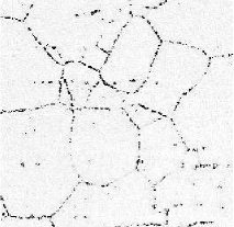
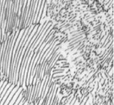
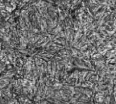
(a)	(b)	(c)

Figure 1: Microscope image of: (a) austenite, (b) perlite and (c) martensite [1].

The outline of the paper is as follows: after explaining the choice of the order parameters for each transformation in Sect.2, in Sect.3 balance equations are provided for linear momentum, solute mass and internal energy; the first two will act as the evolution equations needed for a Ginzburg-Landau framework. In Sect.4 the restrictions provided by the second law of thermodynamics are highlighted and its exploitation in the form of the Clausius-Duhem inequality is provided. In Sect.5 the model is completed with the description of the Helmholtz free energy density, which will allow an explicit form for the constitutive laws to be derived in Sect.6. The resulting model is a diffuse interface one, and this implies the presence of the gradient of the order parameters, which will put some issues regarding the exploitation of the second principle of thermodynamics (Sect.4) and the necessary high order boundary conditions, as highlighted in Sect.6.3. The paper ends drawing some conclusions.

2 Model of the problem

The model is set at a microscopic scale of observation which may be, for instance, a single-grain scale and relies on a number of order parameters to describe the different kinds of transformations involved. In order to account for the presence of three phases (austenite, perlite and martensite), two order parameters playing as the unknowns of the problem may be introduced.

2.1 Diffusive order parameter

To account for diffusive phenomenon, an order parameter called $c$ is set:

$$c=c({\bm{x}},t),\quad{\rm for}\ ({\bm{x}},t)\in\Omega\ \times\ [0,\infty),$$ (1)

being $\Omega$ a two-dimensional domain.

This parameter describes the evolution from one phase to another one with a different structure. According to experimental observations and the use of the Cahn-Hilliard equation [25] (see Sect.3), the order parameter may represent the solute mass fraction. Hence, Pearlite, and in general phases obtained by diffusive transformations, will be the one for which this order parameter is non-zero, i.e. the carbon has migrate to generate areas in which there is a great quantity $(c>0)$ in spite of other areas, in which there is a lack of carbon $(c<0)$. Moreover, the higher value $c$ will assume in a point of the domain, the more the transformation will be at a late stage there. Given this interpretation, the Cahn-Hilliard equation may be seen as a balance of mass equation.

2.2 Displacive order parameter

Regarding martensitic phase formation, a shear strain needs to be applied to the lattice in order to obtain the phase change [20], [21]. For this reason, in considering displacive phenomena, the common choice for the order parameter, called $e_{2}$, in a two-dimensional setting [8] [22] [23] is

$$e_{2}=\frac{\varepsilon_{11}-\varepsilon_{22}}{\sqrt{2}},$$ (2)

where

$${\bm{\varepsilon}}=\frac{1}{2}\left(\nabla{\bm{u}}+\nabla{\bm{u}}^{T}\right)$$ (3)

is the linearised strain tensor and

$$\bm{u}=\bm{u}({\bm{x}},t),\quad{\rm for}\ ({\bm{x}},t)\in\Omega\ \times\ [0,\infty)$$ (4)

is the displacement field.

3 Balance equations

We start the description of the model by stating the balance equations and then by examining the restrictions imposed by the second law of thermodynamics. We will last enter appropriate constitutive hypothesis by choosing a constitutive law for the free energy.

The model consists of three balance equations, reported here in their pointwise formulation:

• balance of linear momentum:

  $$\rho\ddot{\bm{u}}-\nabla\cdot\bm{\sigma}=\rho\bm{f},$$ (5)

  where $\bm{\sigma}$ is the stress tensor and $\bm{f}$ is the external body force;

• balance of solute mass:

  $$\dot{c}=-\nabla\cdot\bm{J},$$ (6)

  where $\bm{J}=c\bm{V}$ is the flux vector related to the solute mass fraction ($\bm{V}$ is its the velocity);

• balance of energy:

  $$\dot{e}=\mathpzc p^{i}_{m}+\mathpzc p^{i}_{c}+h;$$ (7)

  here, $e$ is the internal energy density, $\mathpzc p^{i}_{m}$ is the mechanical internal power (density), $\mathpzc p^{i}_{c}$ is the internal power associated to the solute mass balance equation and $h$ is the internal thermal power. This can be expressed by the thermal power balance

  $$h=-\nabla\cdot\bm{q}+r,$$ (8)

  $\bm{q}$ being the heat flux and $r$ the external heat supply.

The balance of linear momentum and of solute mass give rise to two power balance equations.

To account for non-local effects and spatial variations of the order parameters (interfaces), we demand a non-local constitutive relation for stress and chemical potential. Some cares are needed due to the presence of non-localities in the constitutive equations, as this will lead to non-conventional expressions for the internal powers associated to momentum and solute mass balance.

For the time being it suffices to consider this relation in the quite generic form

$$\bm{\sigma}=\bm{\sigma}_{loc}(\Gamma_{loc},\dot{\Gamma}_{loc})-\nabla\cdot\bm{\Sigma}(\Gamma),$$ (9)

where $\Gamma_{loc}=(\bm{\varepsilon},c,T)$ are the local state variables and $\Gamma=(\Gamma_{loc},\nabla\bm{\varepsilon},\nabla c)$ is the full set of state variables Moreover, $\bm{\sigma}_{loc}$, $\nabla\cdot\bm{\Sigma}$ are supposed to be symmetric second order tensors. The dependence upon $\dot{\Gamma}_{loc}$ accounts for possible dissipative contributions to the local stress; we will not consider dissipative contributions to the non local part of the stress. The balance of mechanical power is obtained by multiplying the balance of linear momentum equation by $\bm{v}=\dot{\bm{u}}$, which leads to

$$\frac{d}{dt}\left(\frac{1}{2}\rho\bm{v}^{2}\right)=[\nabla\cdot(\bm{\sigma}_{loc}-\nabla\cdot\bm{\Sigma})+\bm{f}]\cdot\bm{v}=\\ =-(\bm{\sigma}_{loc}:\dot{\bm{\varepsilon}}+\bm{\Sigma}\vdots\nabla\dot{\bm{\varepsilon}})+\nabla\cdot[\bm{\sigma}\cdot\bm{v}+\bm{\Sigma}:\dot{\bm{\varepsilon}}]+\bm{f}\cdot\bm{v},$$ (10)

having enforced the symmetry condition for the tensors and therefore substituted $\dot{\bm{\varepsilon}}$ with $\nabla\bm{v}$. We interpret (10) as a balance equation for the rate of change of kinetic energy and the internal and external (mechanical) powers:

$$E(\mathcal{S})=\int_{\mathcal{S}}\frac{1}{2}\rho\bm{v}^{2}dw,$$ (11)

$$\mathcal{P}_{m}^{i}({\mathcal{S}})=\int_{\mathcal{S}}(\bm{\sigma}_{loc}:\dot{\bm{\varepsilon}}+\bm{\Sigma}\vdots\nabla\dot{\bm{\varepsilon}})\,dw,$$ (12)

$$\mathcal{P}_{m}^{e}({\mathcal{S}})=\int_{\mathcal{S}}\bm{f}\cdot\bm{v}dw+\int_{\partial{\mathcal{S}}}(\bm{\sigma}\cdot\bm{v}+\bm{\Sigma}:\dot{\bm{\varepsilon}})\cdot\bm{\nu}ds,$$ (13)

where ${\mathcal{S}}$ is any sub-body, $dw$ is the volume measure, $ds$ the surface measure and $\bm{\nu}$ the surface normal. We have used capital letters for the integrated powers, so that $\mathcal{P}_{m}^{i}({\mathcal{S}})=\int_{\mathcal{S}}\mathpzc p_{m}^{i}dw$.

The balance of mechanical power equation is expressed as

$$\dot{E}({\mathcal{S}})+\mathcal{P}_{m}^{i}({\mathcal{S}})=\mathcal{P}_{m}^{e}({\mathcal{S}}).$$ (14)

Now we consider the power associated to the balance of solute mass equation. We call $\mu$ the chemical potential, which is the variable conjugated to $\dot{c}$ defining the power balance associated to (6):

$$\mu\dot{c}=-\mu\nabla\cdot\bm{J}.$$ (15)

A constitutive expression function of $\Gamma$ for the chemical potential has to be given, as well as a non-local relation:

$$\mu=\mu_{loc}(\Gamma_{loc})-\nabla\cdot\bm{M}(\Gamma).$$ (16)

We can rewrite (15) as

$$\mu(\dot{c}+\nabla\cdot\bm{J})=\dot{c}\mu+\nabla\cdot(\mu\bm{J})-\bm{J}\cdot\nabla\mu=\\ (\dot{c}\mu_{loc}+\bm{M}\cdot\nabla\dot{c}-\bm{J}\cdot\nabla\mu)+\nabla\cdot(\mu\bm{J}-\dot{c}\bm{M})=0.$$ (17)

We define the internal and the external powers as follows:

$$\mathcal{P}^{i}_{c}({\mathcal{S}})=\int_{\mathcal{S}}(\dot{c}\mu_{loc}+\bm{M}\cdot\nabla\dot{c}-\bm{J}\cdot\nabla\mu)dw,$$

$$\mathcal{P}^{e}_{c}({\mathcal{S}})=\int_{\partial{\mathcal{S}}}(\dot{c}\bm{M}-\mu\bm{J})\cdot\bm{\nu}ds$$

so that the balance of powers in the sub-volume ${\mathcal{S}}$ is expressed as

$$\mathcal{P}^{i}_{c}({\mathcal{S}})=\mathcal{P}^{e}_{c}({\mathcal{S}}).$$ (18)

Note that there is no energy related to a second order time derivative in the balance of solute mass equation.

4 Restrictions from the Second Law of Thermodynamics

We will examine the restrictions entailed by the second law of thermodynamics in the form of the classical Clausius-Duhem inequality:

$$\dot{\eta}\geq-\nabla\cdot\frac{\bm{q}}{T}+\frac{r}{T}.$$ (19)

By using the first law of thermodynamics (balance of energy equation):

$$\dot{e}=\mathpzc p^{i}_{tot}-\nabla\cdot\bm{q}+r$$ (20)

(where $\mathpzc p^{i}_{tot}\equiv\mathpzc p^{i}_{m}+\mathpzc p^{i}_{c}$ ) to eliminate the source term $r$, and introducing the Helmholtz free energy density $\psi=e-T\eta$, the Clausius-Duhem inequality can be expressed in the more convenient form (reduced inequality)

$$\dot{\psi}+\dot{T}\eta-\mathpzc p^{i}_{tot}\leq-\frac{\bm{q}}{T}\nabla T.$$ (21)

By substituting the expressions for the internal powers and remembering that $\psi$ is a function of the variables $\Gamma=(\bm{\varepsilon},c,T,\nabla\bm{\varepsilon},\nabla c)$, the inequality becomes

$$(\psi_{T}+\eta)\dot{T}+(\psi_{c}-\mu_{loc})\dot{c}+(\psi_{\nabla c}-\bm{M})\cdot\nabla\dot{c}+$$

$$+(\psi_{\nabla\bm{\varepsilon}}-\bm{\Sigma})\vdots\nabla\dot{\bm{\varepsilon}}+(\psi_{\bm{\varepsilon}}-\bm{\sigma}_{loc}):\dot{\bm{\varepsilon}}+\bm{J}\cdot\nabla\mu+\frac{\bm{q}}{T}\cdot\nabla T\leq 0,$$

where the subscripts represent partial derivatives. This inequality has to be satisfied for all processes $(\dot{\bm{\varepsilon}},\dot{c},\dot{T},\nabla\dot{\bm{\varepsilon}},\nabla\dot{c},\nabla\mu,\nabla T)$. Since $\eta$ (as well as $\psi$) depends only on the state, we obtain

$$\eta=-\psi_{T},$$ (22)

by considering processes with only $\dot{T}$ different from zero. Similarly, as also $\mu_{loc}$, $\bm{M}$, $\bm{\Sigma}$ are assumed state-dependent only, we have

$$\mu_{loc}=\psi_{c},$$ (23)

$$\bm{M}=\psi_{\nabla c},$$ (24)

$$\bm{\Sigma}=\psi_{\nabla\bm{\varepsilon}}.$$ (25)

The entropy inequality is therefore reduced to

$$\left[{\psi_{\bm{\varepsilon}}-\bm{\sigma}_{loc}}\right]:\dot{\bm{\varepsilon}}+\bm{J}\cdot\nabla\mu+\frac{\bm{q}}{T}\cdot\nabla T\leq 0.$$ (26)

The current $\bm{J}$ and the heat flux $\bm{q}$ are in general functions of the state and the process. For our purposes it will be sufficient to make the following simple assumptions ensuring the exploitation of the inequality:

$$\bm{\sigma}_{loc}=\psi_{\bm{\varepsilon}}+\bm{\sigma}_{an},\qquad\bm{\sigma}_{an}=\bm{\gamma}:\dot{\bm{\varepsilon}},$$ (27)

$$\bm{J}=-\alpha\nabla\mu,\qquad\alpha(\Gamma)>0,$$ (28)

$$\bm{q}=-\kappa\nabla T,\qquad\kappa(\Gamma)>0,$$ (29)

where $\bm{\gamma}(\Gamma)$ is a positive definite fourth order tensor of which we provide an explicit formulation in Sect. 6.1, $\alpha$ and $\kappa$ are positive coefficients in general dependent on $\Gamma$, more often only on the temperature $T$. The subscript in the symbol $\bm{\sigma}_{an}$ stands for anelastic. The presence of a dissipative term in the local stress provides a damping mechanism for the displacive transition, as showed in Sect. LABEL:res:displ.

We point out that the chemical potential and the non-dissipative part of the stress can be written accounting for their local and non-local parts in terms of functional derivatives of a free energy functional

$$\Psi=\int_{\Omega}\psi(\Gamma)\,dw,$$ (30)

where $\Omega$ is the material domain and $dw$ the material volume measure. Then,

$$\mu=\psi_{c}-\nabla\cdot\psi_{\nabla c}\equiv\frac{\delta\Psi}{\delta c},\qquad\bm{\sigma}-\bm{\sigma}_{an}=\psi_{\bm{\varepsilon}}-\nabla\cdot\psi_{\nabla\bm{\varepsilon}}\equiv\frac{\delta\Psi}{\delta\bm{\varepsilon}},$$ (31)

these definitions being consistent with the choice of the boundary conditions made in Sect.6.3.

It is possible to substitute the constitutive relations in the equation for the internal powers, obtaining the following internal power density:

$$\mathpzc p^{i}_{tot}=(\psi_{\bm{\varepsilon}}+\bm{\sigma}_{an}):\dot{\bm{\varepsilon}}+\psi_{\nabla\bm{\varepsilon}}\vdots\nabla\dot{\bm{\varepsilon}}+\psi_{c}\dot{c}+\psi_{\nabla c}\cdot\nabla\dot{c}+\alpha|\nabla\mu|^{2}=$$ (32)

$$=\dot{\psi}-\dot{T}\psi_{T}+\alpha|\nabla\mu|^{2}+\dot{\bm{\varepsilon}}:(\bm{\gamma}:\dot{\bm{\varepsilon}}).$$ (33)

Besides, by using $\eta=-\psi_{T}$, we have

$$\dot{e}=\frac{d}{dt}(\psi+T\eta)=\dot{\psi}-\dot{T}\psi_{T}-T\dot{\psi_{T}},$$ (34)

so that (20) can be rewritten in term of the free energy as

$$-T\dot{\psi_{T}}=\alpha|\nabla\mu|^{2}+\dot{\bm{\varepsilon}}:(\bm{\gamma}:\dot{\bm{\varepsilon}})+\nabla\cdot(\kappa\nabla T)+r.$$ (35)

This is a thermodynamically consistent framework which will be substantiated with a convenient choice of the free energy $\psi$ (Sect.5).

5 Free energy

Since constitutive equations have been determined by means of derivatives of the free energy, the choice of this latter is a convenient way to characterise the constitutive content of the model. There are two main phenomena involved in the discussion: the diffusive and the displacive transitions, which have to be accounted for at the same time; this is done by exploiting the additivity property of the energy.

The free energy density is written as the sum of different contributions:

$$\psi=\psi_{0}(T)+\psi_{thel}(c,e_{2},T)+\psi_{diff}(c,T)+\psi_{displ}(\bm{\bm{\varepsilon}},T)\\ +\psi_{cpl}(c,e_{2})+\psi_{grad}(\nabla c,\nabla e_{2}),$$ (36)

where:

• $\psi_{0}$ is a term accounting for the background thermal properties of the material (contributing to specific heat);

• $\psi_{thel}$ is a term accounting for the dilatation due to phase transitions and for the contribution of the shear strain;

• $\psi_{displ}$, which is a function of $e_{2}$, accounts for the displacive transition;

• $\psi_{diff}$, which is a function of $c$, accounts for the diffusive transition;

• $\psi_{cpl}$ is a coupling term for the interaction between the two phases;

• $\psi_{grad}$ is a gradient term and accounts for non-local properties and spatial variations of the order parameter.

In the Ginzburg-Landau theory of phase transitions, it is assumed that the free energy density admits a power series expansion with respect to an order parameter.

5.1 Diffusive part of the free energy

The diffusive part of the free energy may be postulated as follows [13]:

$$\psi_{diff}=A\dfrac{c^{4}}{4}+B(T)\dfrac{c^{2}}{2},$$ (37)

where $A$ is a constant. The function $B(T)$ is given by:

$$B(T)=B_{0}\dfrac{T-T_{P}}{T_{P}},$$ (38)

with $B_{0}$ constant and $T_{P}$ the temperature of perlitic phase transition.

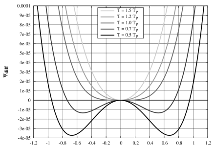
Figure 2: Diffusive free energy.

In Fig.2, $\psi_{diff}$ as a function of $c$ is depicted for various values of temperature. At high temperature there is only one stable phase identified as the minimum for $c=0$, while at low temperature a different stable phase appears for values of $c$ starting from $0$ for $T=T_{P}$ and increasing for decreasing temperature. The transition occurs without hysteresis, i.e. with a continuous variation of the order parameter.

5.2 Displacive part of the free energy

The displacive part of the free energy may be postulated as follows [6], [24]:

$$\psi_{displ}=D\dfrac{e_{2}^{6}}{6}-E\dfrac{e_{2}^{4}}{4}+F(T)\dfrac{e_{2}^{2}}{2},$$ (39)

being $D$, $E$ constants. The function $F(T)$ is given by:

$$F(T)=F_{0}\dfrac{T-T_{M}}{T_{M}},$$ (40)

with $F_{0}$ constant and $T_{M}$ the temperature of martensitic phase transition.

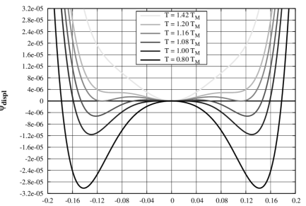
Figure 3: Displacive free energy.

Fig.3 shows that at high temperature only one phase is stable, identified with the minimum for $e_{2}=0$. For $T=T_{M}$ another phase become stable, as the free energy shows two minima. Below the critical temperature, the phase corresponding to the order parameter equal to zero is unstable, whilst the other one, corresponding to non-zero values of $e_{2}$, is stable. Note that, as $e_{2}$ describes a first order phase change, the transition between the phases occurs with a jump in the order parameter.

5.3 Thermo-elastic part of the free energy

The expression of $\psi_{thel}$ is the one for the free energy accounting for the dilatation due to phase transitions [6] [24], changes in temperature and for the contribution of the shear strain.

$$\psi_{thel}=\dfrac{G}{2}\left(e_{1}-x_{1c}c-x_{12}e_{2}^{2}-\beta(T-T_{0})\right)^{2}+\dfrac{H}{2}e_{3}^{2},$$ (41)

being $e_{1}=\dfrac{1}{\sqrt{2}}\left(\varepsilon_{11}+\varepsilon_{22}\right)$, $e_{3}=\varepsilon_{12}$, $G$, $H$, $T_{0}$, $x_{1c}$ and $x_{12}$ constants.

5.4 Coupling part of the free energy

$\psi_{cpl}$ is the coupling free energy and penalises the formation of one low temperature stable phase ($e_{2}\neq 0$ or $c\neq 0$) with respect to the other [6] [24].

$$\psi_{cpl}=x_{2c}c^{2}e_{2}^{2},$$ (42)

being $x_{2c}$ a constant.

5.5 Gradient part of the free energy

The gradient part of the free energy is chosen to be the simplest possible one [6] [24]:

$$\psi_{grad}=K_{e}\dfrac{|\nabla e_{2}|^{2}}{2}+K_{c}\dfrac{|\nabla c|^{2}}{2},$$ (43)

with $K_{e}$ and $K_{c}$ constants; it accounts for non-local effects and spatial variations of the order parameters (interfaces).

6 Summary of the equations of the model

6.1 Constitutive relations: stress and chemical potential

The constitutive laws of stress and chemical potential can be put in an explicit form. It is useful to introduce the following notation:

$$\bm{\epsilon}_{1}=\frac{1}{\sqrt{2}}(\bm{i}\otimes\bm{i}+\bm{j}\otimes\bm{j}),$$ (44)

$$\bm{\epsilon}_{2}=\frac{1}{\sqrt{2}}(\bm{i}\otimes\bm{i}-\bm{j}\otimes\bm{j}),$$ (45)

$$\bm{\epsilon}_{3}=\bm{i}\otimes\bm{j}+\bm{j}\otimes\bm{i}.$$ (46)

The stress tensor can now be written as

$$\bm{\sigma}=\bm{\sigma}_{loc}-(K_{e}\nabla^{2}e_{2})\bm{\epsilon}_{2},$$ (47)

where the local part is given by four contributions:

$$\bm{\sigma}_{loc}=\bm{\sigma}_{displ}+\bm{\sigma}_{thel}+\bm{\sigma}_{cpl}+\bm{\sigma}_{an},$$ (48)

with

$$\bm{\sigma}_{displ}=\left(D{e_{2}}^{5}-E{e_{2}}^{3}+F_{0}\frac{T-T_{M}}{T_{M}}e_{2}\right)\,\bm{\epsilon}_{2},$$ (49)

$$\bm{\sigma}_{thel}=G\left(e_{1}-x_{1c}c-x_{12}e_{2}^{2}-\beta(T-T_{0})\right)(\bm{\epsilon}_{1}-2x_{12}e_{2}\bm{\epsilon}_{2})+He_{3}\bm{\epsilon}_{3},$$ (50)

$$\bm{\sigma}_{cpl}=2x_{2c}c^{2}e_{2}\bm{\epsilon}_{2},$$ (51)

as it regards the conservative contributions; for the dissipative term, we assume

$$\bm{\sigma}_{an}=\gamma\dot{e}_{2}\bm{\epsilon}_{2},$$ (52)

which amounts to consider $\bm{\gamma}=\gamma\bm{\epsilon}_{2}\otimes\bm{\epsilon}_{2}$. In this way, we consider a dissipative term associated only to the displacive order parameter $e_{2}$; its effect is to dim the time oscillations in the order parameter after the displacive transition.

The chemical potential is the following:

$$\mu=\mu_{loc}-K_{c}\nabla^{2}c,$$ (53)

where

$$\mu_{loc}=Ac^{3}+B_{0}\frac{T-T_{P}}{T_{P}}c\\ -Gx_{1c}(e_{1}-x_{1c}c-x_{12}{e_{2}}^{2}-\beta(T-T_{0}))+2x_{2c}{e_{2}}^{2}c.$$ (54)

These expressions have to be substituted in the first two equations of system (59).

6.2 Equations of the model

We now summarise the equations of the model. We collect the three balance equations:

$$\left\{\begin{array}[]{ll}\dot{c}=\nabla\cdot(\alpha\nabla\mu)\\ \rho\ddot{\bm{u}}=\nabla\cdot\bm{\sigma}+\bm{b}\\ c_{s}(T)\dot{T}-T\left[\left(\frac{B_{0}}{T_{P}}c+G\beta x_{1c}\right)\dot{c}+\left(\frac{F_{0}}{T_{M}}+2G\beta x_{12}\right)e_{2}\dot{e}_{2}-G\beta\dot{e}_{1}\right]\\ \qquad\qquad-\alpha|\nabla\mu|^{2}-\gamma\dot{e}_{2}^{2}=\nabla\cdot(\kappa\nabla T)+r,\end{array}\right.$$ (59)

where the last one is the complete heat equation, obtained working out the expression of $\dot{\psi_{T}}$ which appears in eq. (35) and accounting for the anelastic stress $\bm{\sigma}_{an}$ in (52). We remark that

$$c_{s}(T)=-T\psi_{TT}=-T(\,(\psi_{0})_{TT}+G\beta^{2}\,)$$ (60)

denotes the specific heat. The given expression of the heat equation allows to identify the thermo-chemical and the thermo-mechanical coupling terms (contained in the second term of eq. 59₃), which contribute to the changes in temperature during a phase transition, and the chemical and mechanical dissipations, respectively $\alpha|\nabla\mu|^{2}$ and $\gamma\dot{e}_{2}^{2}$, which act as heat sources when a displacive or a diffusive transition occurs.

Note that the first of (59) is the classical Cahn-Hilliard equation [25].

6.3 Boundary and initial conditions for the differential system

Well-posed boundary and initial conditions are necessary to complement Eqs.(59). Let $\Omega$ be the domain in the material description (for the purposes exposed here, no distinction is made between the material particles of the material description and the reference configuration of the referential description). To state the boundary conditions in a general mixed form, we assume that the boundary $\partial\Omega$ is partitioned into two subsets in two different ways:

$$\partial\Omega=\partial\Omega_{s}\cup\partial\Omega_{u}=\partial\Omega_{q}\cup\partial\Omega_{T},$$ (61)

with

$$\partial\Omega_{s}\cap\partial\Omega_{u}=\varnothing,\qquad\partial\Omega_{q}\cap\partial\Omega_{T}=\varnothing.$$ (62)

We assume the following boundary conditions:

$$\left\{\begin{array}[]{ll}{\nabla c(\bm{x},t)\cdot\bm{\nu}}\Big{|}_{\partial\Omega}=0\\ {\nabla\mu(\bm{x},t)\cdot\bm{\nu}}\Big{|}_{\partial\Omega}=0\\ {\nabla e_{2}(\bm{x},t)\cdot\bm{\nu}}\Big{|}_{\partial\Omega}=0\\ {\bm{q}\cdot\bm{\nu}}\Big{|}_{\partial\Omega_{q}}=g(\bm{x})\\ {\bm{\sigma}_{loc}(\bm{x},t)\cdot\bm{\nu}}\Big{|}_{\partial\Omega_{s}}=\bm{t}(\bm{x})\\ {\bm{u}(\bm{x},t)}\Big{|}_{\partial\Omega_{u}}=\tilde{\bm{u}}(\bm{x})\\ {T(\bm{x},t)}\Big{|}_{\partial\Omega_{T}}=\tilde{T}(\bm{x}).\\ \end{array}\right.$$ (70)

We remark that the first and the second conditions ensures the global conservation of solute mass in the domain:

$$\frac{d}{dt}\int_{\Omega}c\,dw=\int_{\partial\Omega}\bm{J}\cdot\bm{\nu}\,ds=0.$$ (71)

The non-local boundary conditions (Eqs.(70)₂, (70)₃) are needed in this model due to the non-local form of the stress [26]. The other conditions are classical.

The initial conditions are the following:

$$\left\{\begin{array}[]{ll}\bm{u}(\bm{x},0)=\bm{u}_{0}(\bm{x})\\ \dot{\bm{u}}(\bm{x},0)=\bm{v}_{0}(\bm{x})\\ c(\bm{x},0)=c_{0}(\bm{x})\\ T(\bm{x},0)=T_{0}(\bm{x}).\end{array}\right.$$ (76)

7 Conclusions

A model to study both diffusive and displacive phase transitions has been proposed in a thermodynamically consistent framework in which, for the presence of the balance of energy equation, non-isothermal conditions can be accounted for. The resulting model is a diffuse interface one, and relies on the choice of two order parameters and of its gradients; this rises some issues about the exploitation of the Clausius-Duhem inequality, and a way to deal with this has been proposed. In particular, we have considered a suitable modification of the first law of thermodynamics by including non-conventional expressions for the internal powers (due to non-localities), keeping at the same time the classical Clausius-Duhem form for the second law of thermodynamics.

The equations of the model are the balance of linear momentum equation, the Cahn-Hilliard equation and the heat equation; the first two are the evolution equations for the two order parameters; the heat equation accounts for thermal effects like cooling or heat released due to a phase change. The model is complemented by a proper description of the free energy and consistent boundary and initial conditions; due to the presence of the gradients of the order parameters, two higher order boundary conditions appear to be necessary, and this can be also observed in the exploitation of the Clausius-Duhem inequality.

References

References

- [1] ASM Metals Handbook - Atlas of microstructures of industrial alloys (Vol.7) American Society for Metals, 1972.
- [2] M. Brokate, J. Sprekels, Hysteresis and Phase Transitions Springer, New York, 1996.
- [3] D. Hoemberg, A mathematical model for the phase transitions in eutectoid carbon steel, IMA J. Appl. Math. 54 (1995) 31-57.
- [4] L.D. Landau, D.M. Lifshitz, Statistical Physics, Pergamon, Oxford, 1968.
- [5] J.C. Toledano, P. Toledano, The Landau Theory of the Phase Transitions, World Scientific Editor, 1987.
- [6] F. Falk, Model free energy, mechanics and thermodynamics of shape memory alloys, Acta Metallurgica 28(1980) 1773-1780.
- [7] G.R. Barsch, J.A. Krumhansl, Twin Boundaries in Ferroelastic Media without Interface Disolcations, Physical Review Letters, 53(1984) 1070-1072.
- [8] R. Ahluwalia, T. Lookman, A. Saxena, Dynamic strain loading of cubic to tetragonal martensites, Acta Materialia 54(2006) 2109-2120.
- [9] V.I. Levitas, D.L. Preston, Three-dimensional Landau theory for multivariant stress-induced martensitic phase transformations I. AusteniteMartensite, Physical Review B 66(2002) 134206-1-9.
- [10] Y. Wang, A.G. Khachaturyan, Three dimensional field model and computer modeling of martensitic transformations, Acta mater. 45(1997), 759-773.
- [11] A. Artemev, Y. Jin and A. Khachaturyan, Three-dimensional phase field model of proper martensitic transformation, Acta Mater. 49(2001) (7), 1165-1177.
- [12] V. Berti, M. Fabrizio, D. Grandi, Phase transitions in shape memory alloys: A non-isothermal Ginzburg-Landau model, Physica D, in press.
- [13] J. Cahn, On spinodal decomposition, Acta Metallurgica, 9(1961) 795-801.
- [14] H.W. Alt, I. Pawlow, A mathematical model of dynamics of non-isothermal phase separation, Physica D 59(1992) 389-416.
- [15] A. Onuki, A. Furukawa, Phase transitions of Binary Alloys with Elastic Inhomogeneity, Physical Review Letters 83(2001) 452-455.
- [16] E. Fried, M.E. Gurtin, Continuum theory of thermally induced phase transitions based on an order parameter, Physica D 68(1993) R 326-343.
- [17] M. Rao, S. Sengupta, Nucleation of Solids in Solids: Ferrites and Martensites Physical Review Letters 91(2003) 045502-1-3.
- [18] V.I. Levitas, Thermomechanical and kinetic approaches to diffusional-displacive phase transitions in inelastic materials, Mechanics Research Communications 27(2000) 217-227.
- [19] M. Bouville, R. Ahluwalia, Effect of lattice-mismatch-induced strains on coupled diffusive and displacive phase transformations, Physical Review B 75(2007) 054110-1-11.
- [20] D.S. Lieberman, M.S. Wechsler, T.A. Read, Cubic to Orthorhombic Diffusionless Phase Change-Experimental and Theoretical Studies of AuCd, Journal of Applied Physics 26(1955) 473-484.
- [21] H.K.D.H. Bhadeshia, Worked examples in the geometry of crystals, The Institute of Metals, London, 1987.
- [22] S.R. Shenoy, T. Lookman, A. Saxena, A.R. Bishop, Martensitic textures: Multiscale consequences of elastic compatibility, Physical Review B 60(1999) R 12-537-541.
- [23] R.C. Albers, R. Ahluwalia, T. Lookman, A. Saxena, Modeling solid-solid phase transformations: from single crystal to polycrystal behaviour, Computational and Applied Mathematics 23(2004) 345-361.
- [24] A. Onuki, Pretransitional Effects at Structural Phase Transitions, J. Phys. Soc. Jpn., 68(1999) 5-8.
- [25] J. Cahn, J.E. Hilliard Free energy of a nonuniform system. I. Interfacial free energy The journal of Chemical Physics, 28(1958) (2) 258-267.
- [26] Polizzotto C. Unified thermodynamic framework for nonlocal/gradient continuum theories, European Journal of Mechanics A/Solids, 22(2003) 651-668.