Magnetic impurity in a $U(1)$-Spin Liquid with a Spinon Fermi-Surface

Abstract

We address the problem of a magnetic impurity in a two dimensional $U(1)$ spin liquid where the spinons have gap-less excitations near the Fermi-surface and are coupled to an emergent gap-less gauge field. Using a large N expansion we analyze the strong coupling behavior and obtain the Kondo temperature which was found to be the same as for a Fermi-liquid. In this approximation we also study the specific heat and the magnetic susceptibility of the impurity. These quantities present no deviations from the Fermi-liquid ones, consistent with the notion that the magnetic impurity is only sensitive to the local density of fermionic states.

I introduction

A large number of theoretical proposals for the low-energy description of spin-liquid phases consider fractionalized fermionic degrees of freedom, the spinons, carrying spin $1/2$ but no electric charge, coupled to an emergent $U(1)$ gauge field, a gap-less photon-like mode. The spinons are gap-less having either nodal points Wen (2002) or a Fermi-surface. The former case arises naturally in the slave particle approach to the $t-J$ model Lee and Nagaosa (1992) but also in other physical contexts such as the half-filled Landau level Halperin et al. (1993) and the description of metals at a Pomeranchuk instability Oganesyan et al. (2001). It presents non-Fermi liquid behavior due to the strong interactions between the spinons and the gauge field that lead to a spectrum with no well defined quasi-particles. This phase has a number of remarkable thermodynamical and transport properties Nave and Lee (2007), for example at low temperatures soft gauge modes contribute to the specific heat with a term proportional to $T^{2/3}\$ Motrunich (2005).

Magnetic impurities embedded in a parent material provide an experimental probe to the bulk properties and can help to discriminate between possible candidate phases. Moreover in order to be observed experimentally the system itself should be stable to a dilute density of such impurities. In a Fermi-liquid an antiferromagnetically coupled spin impurity leads to the well known Kondo effect Hewson (1996) characterized by a cross over from the low temperature strong coupled regime, where the magnetic moment of the impurity is completely screened by the bulk quasi-particles, to the high temperature regime, where the impurity susceptibility follows a Curie-Weiss law. This cross-over occurs near the Kondo temperature which is an example of a dynamically generated energy scale. Since the understanding of the Kondo effect the study of impurities in different bulk phases has attracted much attention Cassanello and Fradkin (1996, 1997); Florens et al. (2006); Kolezhuk et al. (2006); Kim and Kim (2008), in particular for bosonic Florens et al. (2006) and algebraic spin liquids Kolezhuk et al. (2006); Kim and Kim (2008).

The purpose of the present work is to study the behavior of a magnetic impurity embedded in a $U(1)$ spin liquid with a Fermi-surface. Being a charge insulator this system still presents a Kondo like behavior since the spin degrees of freedom are free to screen the magnetic impurity at low energies. The article is organized as follows: in sec.II we describe the model and give some details of the $1/N$ expansion (sec. II.1 and II.2), the specific heat and the local spin susceptibilities are respectively computed in sec. II.3 and II.4. Finally in sec.III we conclude discussing the implications of our results.

II methods

Starting from the $t-J$ model in 2-D, the action describing the spin-liquid phase with a spinon Fermi surface coupled to a compact $U(1)$ gauge field can be obtained within the slave-boson formalism Lee and Nagaosa (1992) or using a slave-rotor representation Lee and Lee (2005), when fluctuations around the mean-field solution are considered. We assume that due to the presence of a large number of gap-less fermions the system is deconfined i.e. one can consider a non-compact $U(1)$ gauge theory Hermele et al. (2004). The partition function writes as a path integral over the spinon grassmanian fields $f_{\sigma=\pm 1}$ and the bosonic gauge fields $a_{\mu}=\left(a_{0},\boldsymbol{a}\right)$ with action

$$\mathcal{S}_{SL} = \int d^{3}x\sum_{\sigma=\pm}\left\{f_{\sigma}^{\dagger}\left(\partial_{\tau}+ia_{0}\right)f_{\sigma}\right.$$

$$\left.+\frac{1}{2m}\left[\left(\boldsymbol{\partial}-i\boldsymbol{a}\right)f_{\sigma}^{\dagger}\right]\mathbf{.}\left[\left(\boldsymbol{\partial}+i\boldsymbol{a}\right)f_{\sigma}\right]-\frac{1}{b}ia_{0}\right\},$$

where $b$ is the microscopic lattice volume and $m$ the spinon mass. The integration over the temporal component of the gauge field $a_{0}$ acts as an on-site chemical potential for the spinons enforcing $b\sum_{\alpha}f_{\alpha}^{\dagger}\,f_{\alpha}=1$. We use the notation$\int d^{3}x=\int_{0}^{\beta}d\tau\int d^{2}x$.

At $\mathbf{x}=\mathbf{0}$ the interaction with the magnetic impurity is given by $\mathcal{S}_{K}=\mathcal{S}_{Berry}+J_{K}b\int d\tau\ \mathbf{S}_{f}(\mathbf{0})\mathbf{.}\mathbf{S}$, where $\mathcal{S}_{Berry}$ is the action of the free impurity spin, $J_{K}$ is the Kondo coupling and $\mathbf{S}_{f}\left(\mathbf{0}\right)=f_{\alpha}^{\dagger}\left(\tau,\mathbf{0}\right)\boldsymbol{\sigma}_{\alpha,\beta}\,f_{\alpha}\left(\tau,\mathbf{0}\right)$. Using a fermionic representation for the impurity spin $\mathbf{S}=c_{\alpha}^{\dagger}\boldsymbol{\sigma}_{\alpha,\beta}\,c_{\alpha}$, this term writes explicitly $\mathcal{S}_{K}=\int d\tau\left\{\sum_{\sigma}c_{\sigma}^{\dagger}\left(\partial_{\tau}+i\lambda\right)c_{\sigma}-i\lambda-J_{K}b\mathbf{S}_{f,0}\mathbf{.}\mathbf{S}\right\},$ where $\lambda$ is an integration parameter inserted in order to enforce the constrain $\sum_{\alpha}c_{\alpha}^{\dagger}\,c_{\alpha}=1$.

II.1 Large N expansion

Perturbative expansions for the Kondo problem are plagued with infrared logarithmic divergences signaling the fact that, for low energy, the system flows to a strong coupled fixed point where the impurity forms a singlet with the bulk electrons. Even if resummation of the divergent terms is possible this method is not well suited to describe the low temperature phase. Alternatively the large $N$ expansion reproduces the essential features of the Kondo effect in the strong coupling regime. However for temperatures of the order of the Kondo temperature $T_{K}$, where a cross over to the asymptotic free regime is expected, this technique becomes unreliable due to the violation of the occupancy constrain and instead predicts a continuous phase transitionBickers (1987). Therefore our results are restricted to the low energy regime. For the $U(1)$ spin liquid the large $N$ expansion corresponds to the random-phase-approximation (RPA) used to obtain most of the physical predictions for this phaseNave and Lee (2007). Recently the validity of this method applied to this specific problem was questioned Lee (2009) since all planar diagrams where shown to contribute to leading order. A possible resolution was proposed in Mross et al. (2010) using a double expansion to control higher loop contributions and essentially recovering the RPA result.

In order to perform a saddle-point expansion we generalize the above action to $su(N)$ following the standard procedureRead and Newns (1983); Cassanello and Fradkin (1996); Bickers (1987): the Pauli matrices $\boldsymbol{\sigma}=\{\sigma_{1},...,\sigma_{3}\}$ are replaced by the generators of $su(N)$ $\boldsymbol{\tau}=\{...,\tau^{a},...\}$ with the index $a=1,..,N^{2}-1$ and the coupling constant is rescaled $J_{K}\to\frac{J_{K}}{N}$. The representation of the impurity spin is taken to be conjugate to the spinons one. Using the Fierz-like identityCassanello and Fradkin (1996) the Kondo term writes

$$\mathcal{S}_{K} = \int d\tau\left\{\sum_{\sigma}c_{\sigma}^{\dagger}\left(\partial_{\tau}+i\lambda\right)c_{\sigma}-i\lambda Q_{f}\right.$$ (2)

$$\left.+\frac{J_{K}}{N}b\left(f_{\alpha}^{\dagger}\left(0\right)c_{\alpha}c_{\beta}^{\dagger}f_{\beta}\left(0\right)\right)+J_{K}\right\},$$

and the last term of Eq. (II) is now multiplied by $Q_{f}$ defined such that $b\sum_{\sigma}f_{\sigma}^{\dagger}\left(\mathbf{x}\right)f_{\sigma}\left(\mathbf{x}\right)=\sum_{\sigma}c_{\sigma}^{\dagger}c_{\sigma}=Q_{f}$ .

Following Read and Newns (1983), the interaction term is decoupled inserting a bosonic Hubbard-Stratonovich field $\chi=\kappa e^{i\phi}$. The integration over $\phi$ can be absorbed by a shift in $\lambda$ leaving a single real dynamical variable $\kappa$. The integration over the fermionic degrees of freedom can then be performed and the partition function writes $Z=\int DaD\lambda D\kappa e^{-N\,s_{b}}$ where

$$s_{b} = -\frac{1}{N}\text{Tr}\ln\left[-G^{-1}\right]-\frac{1}{N}\text{Tr}\ln\left[-F^{-1}\right]+$$ (3)

$$+\int dx_{0}\left\{\frac{1}{J_{K}}\kappa^{2}-i\lambda Q_{f}\right\}-\int d^{3}x\,\frac{Q_{f}}{Nb}ia_{0},$$

is the action for the bosonic fields $a_{\mu}$, $\lambda$ and $\kappa$ only and $F^{-1}$ and $G^{-1}$ are the inverse of the full interacting propagators of the impurity and spinon fermions. We proceed performing a saddle-point expansion in the large $N$ limit imposing the a static ansatz

$$\kappa(\tau) = \kappa_{0}\neq 0,$$ (4)

$$\lambda(\tau) = -i\varepsilon_{c},$$ (5)

$$a_{\mu}(x) = \delta_{0,\mu}\ i\mu.$$ (6)

At $T=0$, the variations of the action in order to $a_{1,2}$ are trivially zero and the ones for $a_{0}$, $\lambda$ and $\kappa$ give, respectively,

$$\frac{1}{\beta}\text{Tr}\left[G_{0}\right] = \frac{V}{b}\frac{Q_{f}}{N},$$ (7)

$$\frac{1}{\pi}\tan^{-1}\left(\frac{\Delta}{\varepsilon_{c}}\right) = \frac{Q_{f}}{N},$$ (8)

$$n(0)b\ln\left(\frac{\Lambda}{\sqrt{\varepsilon_{c}^{2}+\Delta^{2}}}\right) = \frac{1}{J_{K}}.$$ (9)

The first equation fixes the chemical potential $\mu$, where $G_{0}\left(i\omega_{n},\mathbf{k}\right)=\left(i\omega_{n}-\varepsilon_{\mathbf{k}}\right)^{-1}$ is the bare propagator of the spinons with single-particle energies $\varepsilon_{k}=\frac{1}{2m}k^{2}-\mu$. $n(0)=\frac{m}{2\pi}$ is the spinon density of states at the Fermi level and $\Lambda$ is a high-energy cutoff for the dispersion relation. The last two equations were obtained by Read and Newns for the Coqblin-Schriffer Hamiltonian Read and Newns (1983). In the limit where $\Lambda$ is much smaller than the Fermi energy but much larger than the other energy scales the propagator of the impurity fermions is given by $F_{0}\left(i\omega_{n}\right)=\frac{1}{i\omega_{n}-\varepsilon_{c}+i\Delta\text{sgn}\omega_{n}}$ (where $\Delta=\pi n(0)\kappa_{0}^{2}b$) corresponding to a Lorentzian density of states $\rho(\nu)=\frac{1}{\pi}\frac{\Delta}{\left(\nu-\varepsilon_{c}\right)^{2}+\Delta^{2}}$ (see Fig. 4-(a)). The saddle-point values $\varepsilon_{c}$ and $\Delta$ are thus the resonance position and the hybridization width respectively. Identifying the phase shift of an bulk spinon scattered by the impurity $\delta_{f}\left(\omega\right)=\tan^{-1}\left(\frac{\Delta}{\varepsilon_{c}-\omega}\right)$, Eq. (8) is a particular example of the Friedel sum rule. Finally Eq. (9) defines the Kondo energy scale $k_{B}T_{K}=\sqrt{\varepsilon_{c}^{2}+\Delta^{2}}=\Lambda e^{-\frac{1}{b\,n(0)J_{K}}}$. At zero order in $1/N$ there is no influence of the gauge field in the dynamics of the impurity.

A comment about the procedure is in order at this point. One could imagine starting with the bulk theory fixed point obtained in ref.Mross et al. (2010), this would correspond to first renormalize the bulk system propagators and then introduce the impurity. However since $1/N$ is the small parameter of our expansion entering in both the spinon and the impurity Hamiltonians it is natural to start with the bare bulk action. The equivalence of both results can be checked replacing the bare spinon propagator by the integrating one.

II.2 Fluctuations

Fluctuations due to the bosonic fields are obtained summing the fermionic bubbles in the RPA approximation. Without the Kondo term $\left(J_{K}=0\right)$ the propagator $D_{\mu\nu}=\Pi_{\mu\nu}^{-1}$ of the longitudinal and transverse components of the Gauge field is given by the density-density and current-current response functions. Using the Coulomb gauge $\boldsymbol{\nabla}.\boldsymbol{a}=0$ the longitudinal part is fully gaped $\Pi_{00}\simeq\frac{m}{2\pi}$ yielding to screening, by the spinons, of a $U(1)$ test-charge. Therefore one can safely ignore the dynamics of $a_{0}$. The transverse component $\Pi_{i,j}=\left(\delta_{i,j}-\frac{q_{i}q_{j}}{q^{2}}\right)\Pi$ is gap-less and results from the Landau damping of the collective transverse modes by the gap-less spinons. For $\left|\Omega_{u}\right|<v_{F}q$ we can write

$$\Pi\left(i\Omega_{u},\mathbf{q}\right) = \gamma\frac{\left|\Omega_{u}\right|}{q}+\chi q^{2}$$ (10)

where $\gamma=\frac{k_{F}}{\pi}$ and $\chi=\frac{1}{12\pi m}$ Nave et al. (2007).
Using the diagrammatic rules of Fig. 1 the bubble-like diagrams, including transverse gauge as well as $\kappa$ and $\lambda$ fluctuations, are given in Fig. 2 and are divided in pure impurity diagrams, mixed diagrams and gauge diagrams. The transverse component of the gauge vertex is such that $\mathbf{q}\times\boldsymbol{j}=-\frac{1}{m}\mathbf{q}\times\mathbf{k}$.

The impurity diagrams corresponding to the fluctuations of $\kappa$ and $\lambda$ were obtained in ref. Read and Newns (1983) and are given explicitly in the Appendix A.2.

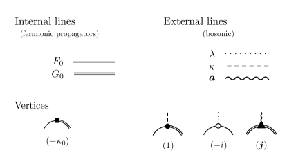
Figure 1: Propagators, vertices and external lines used to obtain the bubble-like diagrams.

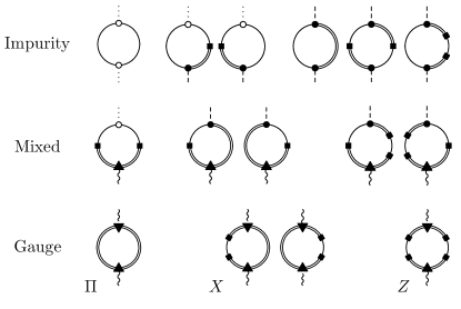
Figure 2: Bubble diagrams obtained summing over the fermionic degrees of freedom. Due to parity mixed diagrams and are evaluated to be zero as well as the one labeled by$Z$.

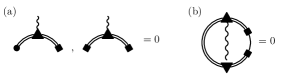
Figure 3: (a) Pieces of diagrams giving zero by parity. (b) $X$ Diagram contributing to the free energy.

It is easy to prove that due to parity considerations all the diagrams including the pieces of Fig.3-(a) are zero (see Appendix A.1). These include the mixed diagrams as well as the ones labeled by $Z$ in Fig. 2. This implies that at this order in the $1/N$ expansion the gauge propagator decouples from the impurity degrees of freedom and the influence of the impurity scattering enters only true the $X$ diagrams contribution:

$$X_{i,j}\left(i\Omega_{u},-\mathbf{q},\mathbf{q}^{\prime}\right)=\frac{1}{\beta}\sum_{n}\int\frac{d\mathbf{k}}{\left(2\pi\right)^{2}}\times$$ (11)

$$b\kappa_{0}^{2}F_{0}\left(i\omega_{n}\right)G_{0}\left(i\omega_{n},\mathbf{k}-\mathbf{q}\right)G_{0}\left(i\omega_{n},\mathbf{k}-\mathbf{q}^{\prime}\right)\times$$

$$\left\{\frac{1}{m}+\frac{\left(\mathbf{k}\times\mathbf{q}\right)_{i}\left(\mathbf{k}\times\mathbf{q}^{\prime}\right)_{j}}{m^{2}\left|\mathbf{q}\right|\left|\mathbf{q}^{\prime}\right|}\left[G_{0}\left(i\omega_{n-u},\mathbf{k}\right)+G_{0}\left(i\omega_{n+u},\mathbf{k}\right)\right]\right\}.$$

Taking into account all non-zero terms the bosonic action (3), developed at Gaussian order, writes now $s_{b}=s_{0}+\frac{1}{N}\left(s_{imp}+s_{a}\right)$, where

$$s_{0} = -\text{Tr}\ln\left[-G_{0}^{-1}\right]-\text{Tr}\,\ln\left[-F_{0}^{-1}\right]$$ (12)

$$+\frac{\beta}{J_{K}}\kappa_{0}^{2}-\varepsilon_{c}\frac{Q_{f}}{N}\beta+\beta\frac{V}{b}\mu\frac{Q_{f}}{N}$$

is the value of the action at the saddle-point, $s_{imp}$ includes the fluctuations of the impurity degrees of freedom (given the original Read and Newns paper Read and Newns (1983) and in Appendix A.2 ) and $s_{a}$ is the action for the transverse component of the gauge field

$$s_{a} = \frac{1}{\beta}\sum_{u}\int\frac{d\mathbf{q}\,d\mathbf{q}^{\prime}}{\left(2\pi\right)^{4}}\,\bar{a}\left(i\Omega_{u},\mathbf{q}\right)a\left(i\Omega_{u},\mathbf{q}^{\prime}\right)\times$$

$$\left[\delta\left(\mathbf{q}-\mathbf{q}^{\prime}\right)\Pi\left(i\Omega_{u},\mathbf{q}\right)+X\left(i\Omega_{u},-\mathbf{q},\mathbf{q}^{\prime}\right)\right],$$

where $\boldsymbol{a}=\hat{\mathbf{q}}_{\perp}a$ and $X_{i,j}=\left(\hat{\mathbf{q}}_{\perp}\right)_{i}\left(\hat{\mathbf{q}^{\prime}}_{\perp}\right)_{j}X$.

II.3 Specific Heat Capacity

We compute the specific heat considering the temperature dependency of the free energy

$$F = -\frac{1}{\beta}\ln Z$$ (13)

$$= \frac{N}{\beta}\left\{s_{0}+\frac{1}{N}\left(\frac{1}{2}\text{Tr}\ln\Gamma+\frac{1}{2}\text{Tr}\ln\left[\Pi+X\right]\right)\right\}.$$

The $s_{0}$ term gives the contribution to the free energy of the bulk fermionic spinons $\left(C_{v}^{\text{(\text{spinon})}}=N\frac{\pi^{2}}{3}Vn(0)T\right)$ and the leading order impurity term $\left(C_{v}^{(\text{imp})}=N\frac{\pi^{2}}{3}\rho(0)T\right)$. The $1/N$ terms carry the free energy contributions from the bosonic degrees of freedom. For low temperature all internal (fermionic) propagators of Fig.2 can be computed at $T=0$ and the temperature dependency is given by the bosonic degrees of freedom Read and Newns (1983). The first next to leading order correction due to the impurity bosons (proportional to $\text{Tr}\ln\Gamma$ in Eq. 13) has been shown to give a correction to the impurity contribution to the specific heat Read and Newns (1983). Defining $C_{v}^{(\text{imp})}=\gamma_{\text{imp}}T$ one obtains $\gamma_{\text{imp}}=\left(N-1\right)\frac{\pi^{2}}{3}\rho(0)$ which can be interpreted as the suppression of one of the $N$ impurity degrees of freedom due to the existence of a constrain.

Since the fluctuations of the gauge and impurity factorize new phenomena can only arise from the $X$ corrections to the propagator of the gauge. In a system with a dilute number of magnetic scatters this term would be of the order of the density of impurities, in this case of a single impurity it is simply proportional to $1/V$. It is therefore natural to expand $\text{Tr}\ln\left[\Pi+X\right]=\text{Tr}\ln\left[\Pi\right]+\text{Tr}\left[\Pi^{-1}X\right]+...$. The first term in the expansion is responsible for the gauge field contribution to the specific heat $C_{v}^{(\text{gauge})}\propto V\left(\frac{\gamma T}{\chi}\right)^{2/3}$. The correction to the free energy $\Delta F=\frac{1}{\beta}\frac{1}{2}\text{Tr}\left[\Pi^{-1}X\right]$ is given by the diagram of Fig. 3-(b). It is easy to prove that such contribution vanishes remarking that one can rewrite it as

$$\frac{1}{\beta}\text{Tr}\left[\Pi^{-1}X\right]=\frac{1}{\beta}\sum_{n}\int\frac{d\mathbf{k}}{\left(2\pi\right)^{2}}\times$$ (14)

$$2b\kappa_{0}^{2}F_{0}\left(i\omega_{n}\right)G_{0}\left(i\omega_{n},\mathbf{k}\right)G_{0}\left(i\omega_{n},\mathbf{k}\right)\Sigma_{f}\left(i\omega_{n}\right)=0$$

where $\Sigma_{f}\left(i\omega_{n}\right)\propto-i\text{sgn}\left(\omega_{n}\right)\left|\omega_{n}\right|^{\frac{2}{3}}$ is the spinon self-energy Mross et al. (2010) given in Fig. 4-(b). The vanishing of such term is a consequence of the independence of $\Sigma_{f}$ from the spinon momentum.

Thus the only correction to the specific heat due to the presence of the impurity is given by a correction to $\gamma^{(\text{imp})}$ since all other terms vanish either by parity considerations of by the above argument.

II.4 Spin Susceptibility

In this section we consider the local spin-spin correlations at the impurity site and its different contributions coming from the impurity-impurity $\chi_{\text{imp},\text{imp}}\left(\tau\right)=\left\langle\mathbf{S}(\tau).\mathbf{S}(0)\right\rangle$ , impurity-spinon $\chi_{\text{imp},\text{spinon}}\left(\tau\right)=\left\langle\mathbf{S}(\tau).\mathbf{S}_{f,(\mathbf{x}=0)}(0)\right\rangle$ and from the local spinon-spinon $\chi_{\text{spinon},\text{spinon}}\left(\tau\right)=\left\langle\mathbf{S}_{f,(\mathbf{x}=0)}(\tau).\mathbf{S}_{f,(\mathbf{x}=0)}(0)\right\rangle$ susceptibilities. In order to investigate the role of the impurity and gauge degrees of freedom we consider the $1/N$ corrections of the propagators and external vertices.

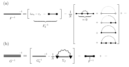
Figure 4: Dyson’s equation for the impurity (a) and spinon (b) propagators up to order $1/N$, for sake of clarity symmetry related diagrams are not shown.

Fig.4 shows diagrammatically the impurity and spinon propagators up to order $1/N$. One can see that to this order the impurity propagator has no corrections due to the presence of the gauge field since terms like $\int d\mathbf{k}\ G_{0}G_{0}\Sigma_{f}=0$ vanish as a consequence of the independence of $\Sigma_{f}$ from the spinon momentum. Alternatively one can use the renormalized spinon propagator to compute the self energy of the impurity (second term of $F_{0}^{-1}$ in Fig.4-(a)) which would correspond to a rearrangement of the terms in 4-(a) leading to the same result. The impurity propagator is thus the same as if the bulk was a regular Fermi-liquid. In this case one can use the results in ref. Read and Newns (1983) where the fluctuations of the bosonic impurity fields $\lambda$ and $\kappa$ were shown to renormalize the Kondo temperature.
Besides the self energy term the spinon propagator, given in Fig. 4-(b), has also a $1/V$ contributions from impurity scattering, these can however be safely ignored in the computation of the local susceptibility since it would give a $1/V^{2}$ correction.

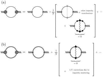
Figure 5: Impurity-impurity and local spinon-spinon spin susceptibilities. The vertex corrections are given to order $1/N$, the bosonic propagators are obtained inverting the bubble like diagrams of Fig. 2. The external zigzag line carry spin and frequency indices.

The impurity-impurity susceptibility is given at leading order in $1/N$ by the bubble diagram of Fig.5-(a) (first term in the r.h.s.). $1/N$ vertex corrections due to the gauge field arising in the impurity-impurity susceptibility also vanish (see Fig.5) since they contain the terms like the ones in Fig.3-(a). One thus concludes that the impurity-impurity susceptibility $\chi_{\text{imp},\text{imp}}$ has no contribution from the gauge field at this order in $1/N$. So the impurity degrees of freedom see only the local density of the spinons, in particular the result given in Read and Newns (1983) for the static susceptibility hold: $\chi_{\text{imp},\text{imp}}\left(i\Omega_{n}=0\right)=\frac{1}{3}J(J+1)(2J+1)\rho\left(0\right)$ where $N=2J+1$.

Gauge contributions are known to enhance Friedel-like oscillations in $U(1)$ spin-liquids Altshuler et al. (1994); Kolezhuk et al. (2006); Mross et al. (2010), this is a consequence of the renormalization of the $2k_{F}$ component of the susceptibility vertex. One could thus expect that the local spinon-spinon susceptibility carried some trace of this behavior. Remarkably no vertex corrections to the local susceptibility due to the gauge field are possible since simple parity arguments like the one used in Appendix A.1 show that the contribution given by the second diagram in the r.h.s of Fig.3-(b) vanishes.

Finally the crossed impurity-spinon susceptibility can also be shown to remain unaffected by the presence of the gauge field using the same simple arguments.
This shows that the local measurements of the susceptibility at the impurity site are insensitive to the gauge degrees of freedom.

III Discussion

We considered the Kondo screening in a bulk system of spinons strongly interacting with a $U(1)$ gauge field. While it is remarkable that Kondo screening can occur for a charge insulator, the results obtained here predict that no particular signature due to the presence of the gauge field can be measured if only the impurity degrees of freedom or local magnetic properties are monitored at the impurity site.

The presence of the impurity destabilizes spin-liquid phase locally and Friedel-like oscillations are expected once the density of spinons is locally disturbed. This is due to the last term in 4-(b), however they would equally be present if the density of spinons was changed by non-magnetic means as for example at the sample edges or near non-magnetic impurities. Such oscillations should be enhanced by the presence of the gauge fields Mross et al. (2010) however they are non-local measures. Local probes will be incapable of distinguish the bulk system from a Fermi-liquid. In particular the Wilson ratio $R=\frac{\pi^{2}\chi_{\text{imp},\text{imp}}\left(0\right)}{J(J+1)\gamma_{imp}}=\frac{N}{N-1}$ for this case is the same as for a magnetic impurity embedded in a Fermi-Liquid Read and Newns (1983).

Appendix A Some details

A.1 Prove that the diagram of Fig.3-(a) is zero

The diagram of Fig. 3-(a) is given by

$$W = b\kappa_{0}^{2}\int\frac{d\mathbf{k}}{\left(2\pi\right)^{2}}G_{0}\left(i\omega_{n},\mathbf{k}\right)\frac{\left(\mathbf{k}\times\mathbf{q}\right)}{m\left|\mathbf{q}\right|}G_{0}\left(i\omega_{n-u},\mathbf{k}-\mathbf{q}\right).$$

Changing variables $\mathbf{k}\to\mathbf{k}^{\prime}=2\frac{\mathbf{q}.\mathbf{k}}{\mathbf{q.q}}\mathbf{q}-\mathbf{k}$, where $\mathbf{k}^{\prime}$ is obtained reflecting $\mathbf{k}$ on axes $\mathbf{q}$ (see Fig.6), leaves the norms $\left|\mathbf{k}\right|=\left|\mathbf{k}^{\prime}\right|$ and $\left|\mathbf{k}-\mathbf{q}\right|=\left|\mathbf{k}^{\prime}-\mathbf{q}\right|$ invariant and changes the sign of $\mathbf{k}\times\mathbf{q}=-\mathbf{k}^{\prime}\times\mathbf{q}$. Since $G_{0}\left(i\omega_{n},\mathbf{k}\right)=G_{0}\left(i\omega_{n},\left|\mathbf{k}\right|\right)$ for a spherically symmetric Fermi surface it follows that $W=-W=0$.

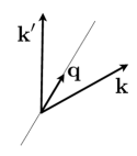
Figure 6: Change of variables that implies that the diagram in Fig.3-(a) is zero.

A.2 Impurity Fluctuation

The impurity action at Gaussian level is given by

$$s_{imp} = \frac{1}{\beta}\sum_{n}\frac{1}{2}\left[\begin{array}[]{c}\bar{\kappa}(i\Omega_{u})\\ \bar{\lambda}(i\Omega_{u})\end{array}\right]^{T}\boldsymbol{\Gamma}(i\Omega_{u})\left[\begin{array}[]{c}\kappa(i\Omega_{u})\\ \lambda(i\Omega_{u})\end{array}\right]$$

where

$$\boldsymbol{\Gamma}(i\Omega_{u}) = \left[\begin{array}[]{cc}\frac{\delta^{2}s}{\delta\bar{\kappa}\delta\kappa}&\frac{\delta^{2}s^{\prime}}{\delta\bar{\lambda}\delta\kappa}\\ \frac{\delta^{2}s^{\prime}}{\delta\bar{\lambda}\delta\kappa}&\frac{\delta^{2}s^{\prime}}{\delta\bar{\lambda}\delta\lambda}\end{array}\right]$$

is the fluctuation matrix. If one evaluate the fermionic Matsubara sums at zero temperature its entries are given by

$$\delta_{\bar{\lambda}}\delta_{\lambda}s = \frac{\Delta}{\pi\left|\Omega_{n}\right|\left(2\Delta+\left|\Omega_{n}\right|\right)}\ln\left[\frac{\varepsilon_{c}^{2}+\left(\left|\Omega_{n}\right|+\Delta\right)^{2}}{\varepsilon_{c}^{2}+\Delta^{2}}\right];$$

$$\delta_{\bar{\lambda}}\delta_{\kappa}s = \frac{2ibn(0)\kappa_{0}}{\left|\Omega_{n}\right|}\left[\tan^{-1}\left(\frac{\left|\Omega_{n}\right|+\Delta}{\varepsilon_{c}}\right)-\tan^{-1}\left(\frac{\Delta}{\varepsilon_{c}}\right)\right];$$

$$\delta_{\bar{\kappa}}\delta_{\kappa}s = bn(0)\left(\frac{2\Delta}{\left|\Omega_{n}\right|}+1\right)\ln\left[\frac{\varepsilon_{c}^{2}+\left(\left|\Omega_{n}\right|+\Delta\right)^{2}}{\varepsilon_{c}^{2}+\Delta^{2}}\right].$$

References

• Wen (2002) X.-G. Wen, Phys. Rev. B 65, 165113 (2002).
• Lee and Nagaosa (1992) P.ย A. Lee and N.ย Nagaosa, Phys. Rev. B 46, 5621 (1992).
• Halperin etย al. (1993) B.ย I. Halperin, P.ย A. Lee, and N.ย Read, Phys. Rev. B 47, 7312 (1993).
• Oganesyan etย al. (2001) V.ย Oganesyan, S.ย A. Kivelson, and E.ย Fradkin, Phys. Rev. B 64, 195109 (2001).
• Nave and Lee (2007) C.ย P. Nave and P.ย A. Lee, Phys. Rev. B 76, 235124 (2007).
• Motrunich (2005) O.ย I. Motrunich, Phys. Rev. B 72, 045105 (2005).
• Hewson (1996) A.ย C. Hewson, The Kondo Problem to Heavy Fermions (Cambridge University Press, Cambridge England, 1996).
• Cassanello and Fradkin (1996) C.ย R. Cassanello and E.ย Fradkin, Phys. Rev. B 53, 15079 (1996).
• Cassanello and Fradkin (1997) C.ย R. Cassanello and E.ย Fradkin, Phys. Rev. B 56, 11246 (1997).
• Florens etย al. (2006) S.ย Florens, L.ย Fritz, and M.ย Vojta, Phys. Rev. Lett. 96, 036601 (2006).
• Kolezhuk etย al. (2006) A.ย Kolezhuk, S.ย Sachdev, R.ย R. Biswas, and P.ย Chen, Phys. Rev. B 74, 165114 (2006).
• Kim and Kim (2008) K.-S. Kim and M.ย D. Kim, J. Phys.: Condens. Matter 20, 125206 (2008).
• Lee and Lee (2005) S.-S. Lee and P.ย A. Lee, Phys. Rev. Lett. 95, 036403 (2005).
• Hermele etย al. (2004) M.ย Hermele, T.ย Senthil, M.ย P.ย A. Fisher, P.ย A. Lee, N.ย Nagaosa, and X.-G. Wen, Phys. Rev. B 70, 214437 (2004).
• Bickers (1987) N.ย E. Bickers, Rev. Mod. Phys. 59, 845 (1987).
• Lee (2009) S.-S. Lee, Phys. Rev. B 80, 165102 (2009).
• Mross etย al. (2010) D.ย F. Mross, J.ย McGreevy, H.ย Liu, and T.ย Senthil, A controlled expansion for certain non-fermi liquid metals, arXiv:1003.0894v1 (2010).
• Read and Newns (1983) N.ย Read and D.ย M. Newns, J. Phys. C 16, 3273 (1983).
• Nave etย al. (2007) C.ย P. Nave, S.-S. Lee, and P.ย A. Lee, Phys. Rev. B 76, 165104 (2007).
• Altshuler etย al. (1994) B.ย L. Altshuler, L.ย B. Ioffe, and A.ย J. Millis, Phys. Rev. B 50, 14048 (1994).