A model of interacting holographic dark energy at the Ricci’s scale

Abstract

We study a holographic cosmological model in which the infrared cutoff is set by the Ricci’s length and dark matter and dark energy do not evolve on their own but interact non-gravitationally with each other. This greatly alleviates the cosmic coincidence problem because the ratio between both components does not vanish at any time. We constrain the model with observational data from supernovae, cosmic background radiation, baryon acoustic oscillations, gas mass fraction in galaxy clusters, the history of the Hubble function, and the growth function.

I Introduction

The efforts made to unveil the nature of dark energy (DE) -the mysterious agent behind the present phase of cosmic accelerated expansion- have been scarcely rewarded so far. We only know by certain that DE is endowed with a hugely negative pressure (of the order of its energy density) and we have grounds to suspect that it is distributed rather evenly across space -see recentreviews to learn about the state of the art.

In view of its mysterious nature many authors have suggested that dark energy should comply with the holographic principle which asserts that the number of relevant degrees of freedom of a system dominated by gravity must vary as the area of the surface bounding the system gerard-leonard . In addition, the energy density of any given region should be bounded by that ascribed to a Schwarzschild black hole that fills the same volume cohen . Mathematically this condition reads $\rho_{X}\leq M_{P}^{2}\,L^{-2}$, where $\rho_{X}$ and $L$ stand for the DE density and the size of the region (or infrared cutoff), respectively, and $M_{P}=(8\pi G)^{-1/2}$ is the reduced Planck mass. This expression is most frequently written in its saturated form

$$\rho_{X}=\frac{3M_{P}^{2}\,c^{2}}{L^{2}}\,.$$ (1)

Here $c^{2}$ is a dimensionless parameter -very often, assumed constant- that summarizes the uncertainties of the theory (such as the number particle species and so on), and the factor $3$ was introduced for mathematical convenience. An interesting feature of holography lies in its close connection to the spacetime foam jng . For additional motivations of holographic dark energy see section 3 of cqg-wd . At any rate, it is sobering to bear in mind that the holographic proposal is just a reasonable hypothesis (which we adopt in this paper) but not necessarily a compelling one.

When dealing with holographic DE one must first specify the infrared cutoff. In the lack of a clear guidance different expressions have been adopted. The most relevant ones are the Hubble radius, i.e., $L=H^{-1}$, see e.g. hubbleradius - and the Ricci’s length, i.e., $L=(\dot{H}+2H^{2})^{-1/2}$ -see e.g. gao ; lxu ; suwa ; lepe . The rationale behind the latter is that it corresponds to the size of the maximal perturbation leading to the formation of a black hole brustein . The radius of the future event horizon have been profusely used but it suffers from a severe circularity problem.

The aim of this paper is to present a cosmological model of holographic dark energy and constrain it with observational data. The model takes the Ricci’s length as infrared cutoff and assumes that dark matter (DM) and dark energy do not evolve separately but interact non-gravitationally with one another. The interaction, albeit proposed just at a phenomenological level, is key to alleviate the coincidence problem luca ; srd which cannot find explanation in the $\Lambda$CDM model and afflicts so many models of evolving DE. On the other hand, recently it has been suggested that the dynamics of galaxy clusters can be better explained if the said interaction is taken into account abdalla-abramo , and it has been invoked to explain the nearly lack of correlation between the orientations of cluster galaxy distributions with those of the underlying dark matter distributions lee . Further, the interaction -first proposed to lower down the theoretical value of the cosmological constant wetterich - is not only necessary but inevitable jerome .

This paper is organized as follows. Section II introduces the model. Section III discusses why Ricci’s holographic models seems to solve the coincidence problem also in the absence of interaction. Section IV presents the statistical analysis of the model after constraining it with data from supernovae type Ia (SN Ia), the shift of the first acoustic peak of the cosmic background radiation (CMB-shift), baryon acoustic oscillations (BAO), gas mass fraction in galaxy clusters, the history of the Hubble parameter, $H(z)$, and the growth function. Lastly, section V briefly delivers our main conclusions and offers some final remarks. As usual, a zero subscript means the present value of the corresponding quantity.

II The holographic model

This model assumes a spatially flat homogeneous and isotropic universe dominated by DM and DE (subscripts $M$ and $X$, respectively), the latter obeying the holographic relationship (1). In virtue of Friedmann equations,

$$H^{2}=\frac{1}{3}M_{P}^{-2}(\rho_{M}\,+\,\rho_{X})\,,$$ (2)

and

$$\dot{H}=-\frac{1}{2}M_{P}^{-2}(\rho_{M}\,+\,\rho_{X}+p_{X})\,,$$ (3)

the fractional DE density, $\Omega_{X}=\frac{\rho_{X}}{3M_{P}^{2}H^{2}}$, can be expressed as

$$\Omega_{X}=\frac{c^{2}}{3c^{2}w+2}\,,$$ (4)

where $w=p_{X}/\rho_{X}$ denotes the equation of state parameter of dark energy which in general depends on time.

The deceleration parameter $q=-\ddot{a}/(a^{2}H^{2})$ takes the simple expression,

$$q=1-\frac{\Omega_{X}}{c^{2}}\,.$$ (5)

As we shall see, as a consequence of the evolution of $\Omega_{X}$, it goes monotonously from positive values at early times (in the matter dominated era) to negative values at later times (in the dark energy dominated era).

The evolution of $\Omega_{X}$ follows from the conservation equations of DE and DM. In the absence of non-gravitational interactions between them they evolve independently and obey

$$\dot{\Omega}_{M}-\left(1-\frac{2\Omega_{X}}{c^{2}}\right)(1-\Omega_{X})\,H = 0\,,$$ (6)

$$\dot{\Omega}_{X}+\left(1-\frac{2\Omega_{X}}{c^{2}}\right)(1-\Omega_{X})\,H = 0\,.$$ (7)

Bearing in mind that in our case $\Omega_{M}\,+\,\Omega_{X}=1$, we get the following expressions in terms of the redshift ($z=a^{-1}-1$),

$$\Omega_{X}=\frac{2\Omega_{X0}-c^{2}+c^{2}(1-\Omega_{X0})(1+z)^{\frac{2}{c^{2}}-1}}{2\Omega_{X0}-c^{2}+2(1-\Omega_{X0})(1+z)^{\frac{2}{c^{2}}-1}}\,.$$ (8)

A very useful quantity when considering the coincidence problem is the ratio between the energy densities, $r=\rho_{M}/\rho_{X}$, which for spatially flat universes reduces to $\Omega_{M}/\Omega_{X}$. The coincidence problem gets alleviated if for reasonable values of $\Omega_{X0}$ and $c^{2}$ we get $r_{0}\sim{\cal O}(1)$. This is the case here since for $\Omega_{X0}$ and $c^{2}$ of order unity, $r_{0}$ also results of this same order. However, for late times (i.e, when $z\rightarrow-1$) one has $r\rightarrow 0$. In this sense, the coincidence problem is not properly solved. To obtain a non-vanishing ratio at late times some interaction between DM and DE must be incorporated in the picture prd-lad .

If DM and DE interact non-gravitationally with each other the evolution equations may be generalized as

$$\dot{\Omega}_{M}-\left(1-\frac{2\Omega_{X}}{c^{2}}\right)(1-\Omega_{X})\,H = QH\,,$$ (9)

$$\dot{\Omega}_{X}+\left(1-\frac{2\Omega_{X}}{c^{2}}\right)(1-\Omega_{X})\,H = -QH\,,$$ (10)

where the Hubble factor on the right hand sides has been introduced to render the interaction term, $Q$, dimensionless.

Since the nature of both dark components is largely unknown, there is ample latitude in choosing $Q$. We shall specify it by demanding that $r$ evolves from an unstable fixed point in the far past, $r_{\infty}\equiv r(z\rightarrow\infty)$, to a stable fixed point at the far future, $r_{f}\equiv r(z\rightarrow-1)$ ladw .

The pair of equations (9) and (10) imply

$$\dot{r}=\left[r\left(1+r-\frac{2}{c^{2}}\right)+Q(1+r)^{2}\right]H\,.$$ (11)

Imposing that $r_{f}$ be a fixed point, i.e., $\dot{r}|_{r=r_{f}}=0$ the interaction term $Q$ is simply a constant given by

$$Q=-\frac{r_{f}}{(1+r_{f})^{2}}\left(1+r_{f}-\frac{2}{c^{2}}\right)\,.$$ (12)

As we shall see later, $r_{f}$ and $c^{2}$ take values such that $Q$ is positive-definite, which entails a transfer of energy from dark energy to dark matter. Obviously if $Q$ were negative, the transfer of energy would go in the opposite direction which would conflict with the second law of thermodynamics db-grg and the coincidence problem would only worsen.

Rewriting Eq. (11) as

$$\dot{r}=(Q+1)(r-r_{f})(r-r_{\infty})H$$ (13)

and using the condition $\dot{r}=0$, the other fixed point can be expressed in terms of the previous one, namely,

$$r_{\infty}=\frac{2-c^{2}(1+r_{f})}{2r_{f}+c^{2}(1+r_{f})}.$$ (14)

To study the stability of the fixed points we first write $r{{}^{\prime}}\equiv dr/d\ln a=\dot{r}/H$ and calculate the derivative of $r{{}^{\prime}}$ with respect to $r$. In the case of the far future fixed point we get

$$\frac{dr^{\prime}}{dr}|_{r_{f}}=1+\frac{2(r_{f}-1)}{c^{2}(r_{f}+1)}\,.$$ (15)

Since $r_{f}$ must be lower than $r_{0}\simeq 0.45$, from Eq. (5) with $c^{2}<\Omega_{X0}\simeq 0.75$ (otherwise $q_{0}$ would not be negative), one follows that $\frac{dr^{\prime}}{dr}|_{r_{f}}<0$, i.e., the fixed point $r_{f}$ is a stable one. Similarly, we find that

$$\frac{dr^{\prime}}{dr}|_{r_{\infty}}=-\frac{2+c^{2}}{c^{2}}+\frac{4}{c^{2}(1+r_{f})}>0\,,$$ (16)

i.e., the fixed point at the far past is an unstable one.

Equation (13) can be integrated with the help of (12). In terms of the redshift it yields,

$$r=\frac{r_{f}(r_{0}-r_{\infty})-r_{\infty}(r_{0}-r_{f})(1+z)^{(Q+1)(r_{\infty}-r_{f})}}{(r_{0}-r_{\infty})-(r_{0}-r_{f})(1+z)^{(Q+1)(r_{\infty}-r_{f})}}\,.$$ (17)

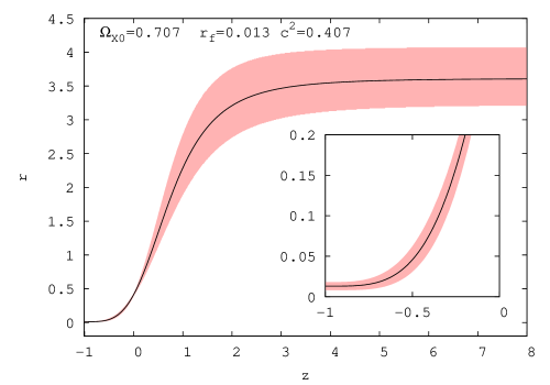
Figure 1: The ratio $r$ between the energy densities vs. redshift for the best fit model. As the inset shows $r_{f}\equiv r(z\rightarrow-1)$ does not vanish. In this, as well as in subsequent figures, the red swath indicates the region obtained by including the $1\sigma$ uncertainties of the constrained parameters used in the calculation.

Inspection of (13) readily shows that when $r$ lies between both fixed points one has $\dot{r}<0$, i.e., the ratio between the energy densities diminishes monotonously from one fixed point to the other. This is depicted in Fig. 1. The said ratio smoothly decreases from high $z$ (i.e., from $r_{\infty}$ -the unstable fixed point is at $z\rightarrow\infty)$) to asymptotically approach the fixed stable point, $r_{f}$, at $z=-1$. Note that the latter needs not be zero. In this regard the coincidence problem is much alleviated because we are not living in any special era. However, the problem is not solved in full since the model cannot predict that $r_{0}$ is of order unity. To the best of our knowledge, no model predicts that, as well as no model predicts the present value of the temperature of the cosmic background radiation, the Hubble constant, or the age of the Universe. For the time being, we must content ourselves by taking these values as input parameters since, very possibly, we are to wait for a successful theory of quantum gravity to compute them.

The expression for the fractional density of dark energy follows from the relationship $r=(1-\Omega_{X})/\Omega_{X}$ and Eq. (17),

$$\Omega_{X}=\frac{(r_{0}-r_{\infty})-(r_{0}-r_{f})(1+z)^{(Q+1)(r_{\infty}-r_{f})}}{(r_{f}+1)(r_{0}-r_{\infty})-(r_{\infty}+1)(r_{0}-r_{f})(1+z)^{(Q+1)(r_{\infty}-r_{f})}}\,.$$ (18)

From the latter and (4) we obtain the equation of state of dark energy in terms of the redshift,

$$w=\frac{1}{3}\left(1-\frac{2}{c^{2}}+r_{\infty}+\frac{(r_{0}-r_{\infty})(r_{\infty}-r_{f})}{r_{\infty}-r_{0}+(r_{0}-r_{f})(1+z)^{(Q+1)(r_{\infty}-r_{f})}}\right)\,.$$ (19)

As shown in the left panel of Fig. 2 for the best fit model, $w$ smoothly evolves from a negative value close to zero at high redshifts to a value lower than $-1$ at the far future. The right panel depicts its evolution near the present time ($z=0$) showing compatibility with recent observational data which suggest that $w$ does not depart much from $-1$ at sufficiently low redshifts (see serra-prd ).

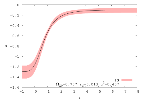
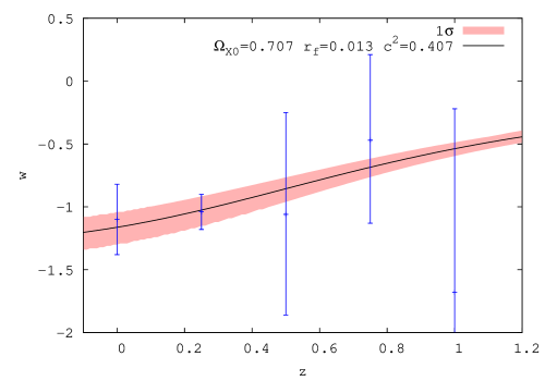
Figure 2: The equation of state parameter (as given by Eq. (19)) vs. redshift up to $z=8$ (left panel), and up to $z=1.2$ only (right panel) for the best fit holographic model. At high redshifts $w$ approaches the equation of state of non-relativistic matter and at low redshifts it does not depart significantly from $-1$. The observational data are taken from serra-prd ; each error bar signifies a $2\sigma$ uncertainty.

Integration of the second Friedmann’s equation (3) provides us with the evolution equation for the Hubble factor which is key to perform the statistical analysis of section IV,

$$H=H_{0}\left[\frac{A_{1}+2\left(A_{2}+(r_{f}-r_{0})(1+z)^{-A_{3}}\right)}{A_{4}}\right]^{1/2}(1+z)^{A_{5}}\,,$$ (20)

where

$$A_{1}=c^{2}(1+r_{f})(1+r_{0})\,,\;\;A_{2}=r_{0}r_{f}-1\,,\;\;A_{3}=1+\frac{2(r_{f}-1)}{c^{2}(1+r_{f})}\,,$$

$$A_{4}=[c^{2}(1+r_{f})+2(r_{f}-1)](1+r_{0})\,,\;\;\;A_{5}=2-\frac{1}{c^{2}(1+r_{f})}.$$

Figure 3 depicts the evolution of the deceleration parameter, Eq. (5), for the best fit model. The observational data are borrowed from Daly . The redshift at which the universe starts accelerating is $z(q=0)=0.56^{+0.12}_{-0.9}$ while for the $\Lambda$CDM model $z(q=0)=0.79\pm 0.02$.

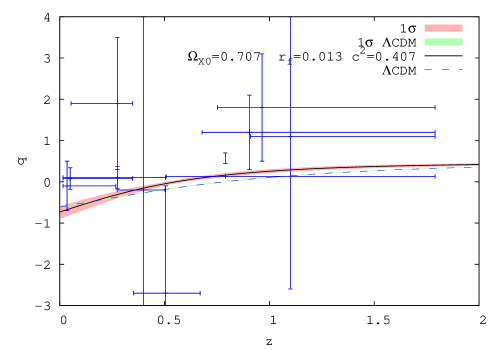
Figure 3: The deceleration parameter vs. redshift for the best fit holographic model (solid line) and the $\Lambda$CDM model (dashed line). In this, as well as in subsequent figures, the green swath indicates the region obtained by including the $1\sigma$ uncertainties of the constrained parameters used in the calculation (in the present case just $\Omega_{M0}$). The observational data are taken from Daly ; however, in view of the large error bars we do not use these data to fit the models.

As mentioned above, there is ample freedom in the choice of the interaction term $Q$. In a previous paper of two of us, on a holographic dark energy model with the Hubble rate as infrared cutoff, we took $Q\propto\Omega_{X}$ id-jcap . We do not pursue this possibility here because, as we have checked, it leads to a universe in which dark energy is subdominant at very late times. While this does not contradict observation, it looks a bit odd. In any case, it deserves a separate study which lies beyond the scope of this paper.

II.1 Age problem

Some cosmological models suffer from the so-called “age problem”, namely, the existence of high redshifts objects whose age at some redshift seem to exceed the Universe’s age predicted at that redshift (as in the $\Lambda$CDM model, see e.g. ademir ).

The age of the Universe at redshift $z$ is

$$t(z)=t_{0}-\int^{z}_{0}\frac{dz^{\prime}}{(1+z^{\prime})\,H(z^{\prime})}\,.$$ (21)

Figure 4 shows the age of the Universe as a function of redshift for the best fit holographic model and the $\Lambda$CDM. Also marked in the figure are the ages and redshifts of three luminous old objects: galaxies LBDS 53W069 ($z=1.43$, $t=4.0$ Gyr) dunlop_1999 and LBDS 53W091 ($z=1.55$, $t=3.5$ Gyr) dunlop_1996 ; spinrad , as well as the quasar APM 08279+5255 ($z=3.91$, $t=2.1$ Gyr) hasinger ; ademir . As is apparent, the ages of two first old objects result compatible with both, the holographic and the $\Lambda$CDM model; however, the age of the old quasar falls only within $2\sigma$ with the ages predicted by these two models. Thus, some tension exists in this regard. By contrast, the interacting holographic model of Ref. id-jcap , which takes as infrared cutoff the Hubble radius, is free of the problem. At any rate, it remains to be seen in which direction (if any) future observations will “move” the age of the said quasar.

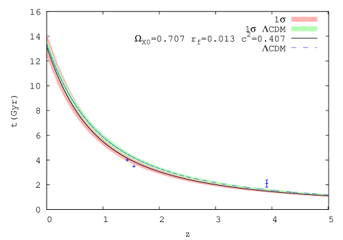
Figure 4: Age of the Universe, $t$, in Giga-years vs. redshift. The solid line corresponds to the best fit holographic model and the dashed line to the $\Lambda$CDM model. The data points from left to right locate the old objects LBDS 53W069, LBDS 53W091 and APM 08279+5255.

III Discussion of the cosmic coincidence

In holographic models of dark energy that take the Ricci’s length as the infrared cutoff one can obtain a finite and approximate constant ratio $r$ for an ample redshift span even if no interaction between the dark components is assumed -see e.g. gao . Here we analyze how this comes about, and we note that while this approach alleviates the coincidence problem it does so only partially since it would entail that we are living in a special time.

We start by rewriting Friedmann’s equation (2) with the help of the saturated holographic bound, $\rho_{X}=3M_{P}^{2}c^{2}\,(\dot{H}+2H^{2})$, as

$$3H^{2}=3c^{2}(\dot{H}+2H^{2})+\frac{\rho_{M0}}{M_{P}^{2}}\,(1+z)^{3}\,,$$ (22)

and, for convenience, introduce the ancillary variable $y^{-\alpha}=1+z$. Thus, Eq. (22) takes the form

$$3\alpha^{2}\frac{\dot{y}^{2}}{y^{2}}=3c^{2}\left\{\alpha\left[\frac{\ddot{y}}{y}-\frac{\dot{y}^{2}}{y^{2}}\right]+2\alpha^{2}\frac{\dot{y}^{2}}{y^{2}}\right\}+\frac{\rho_{M0}}{M_{P}^{2}}\,y^{-3\alpha}\,.$$ (23)

By equating coefficients, we get $\alpha=c^{2}/(2c^{2}-1)$, and

$$\ddot{y}+\frac{\rho_{M0}}{3c^{2}M_{P}^{2}\,\alpha}y^{-3\alpha+1}=0\,.$$ (24)

Multiplying the latter by $\dot{y}$ the differential equation can be readily solved. Upon reverting to the original variable we obtain

$$3H^{2}=\frac{2}{(2-c^{2})M_{P}^{2}}\rho_{M0}(1+z)^{3}+\beta\,M_{P}^{-2}\rho_{M0}(1+z)^{2\frac{1-2c^{2}}{c^{2}}}\,,$$ (25)

where $\beta$ is a positive-definite integration constant that can be identified as $\beta=\left(\frac{1}{r_{0}}\,-\,\frac{c^{2}}{2\,-\,c^{2}}\right)$ and, of the order of unity since $r_{0}$ and $c^{2}$ lie not far from $0.4$.

Recalling Eq. (2) we finally get

$$\rho_{X}=\frac{c^{2}}{2-c^{2}}\rho_{M0}(1+z)^{3}+\beta\,\rho_{M0}\,(1+z)^{2\frac{1-2c^{2}}{c^{2}}}\,.$$ (26)

The DE density is contributed by two terms. The first one redshifts exactly as non-relativistic matter. The second one, in view that $c^{2}$ is bounded by $0.36<c^{2}<0.8$, results subdominant for $z$ of order of unity and larger. Therefore, we can safely conclude that $r=\rho_{M}/\rho_{X}\simeq(2-c^{2})/c^{2}$ for $0\leq z$. This is why the ratio $r$ results of order unity in an ample redshift interval, also in the absence of interaction, as in Ref. gao . However, in view of the observational lower bound on $c^{2}$, we see that $r\rightarrow 0$ as $z\rightarrow-1$. So, in the holographic non-interacting model, $r$ results well below unity, close to zero, and approaches this null value asymptotically for an infinite span of time. Altogether, according to this model, we live in a very special and transient period in which $r$ results comparable to unity.

IV Observational constraints

To constrain the four free parameters ($\Omega_{X0}$, $c^{2}$, $r_{f}$, and $H_{0}$) of the holographic model presented above we use observational data from SN Ia (557 data points), the CMB-shift, BAO, and gas mass fractions in galaxy clusters as inferred from x-ray data (42 data points), the Hubble rate (15 data points), and the growth function (5 data points). Being the likelihood function defined as ${\cal L}\propto\exp(-\chi^{2}/2)$ the best fit follows from minimizing the sum $\chi^{2}_{\rm total}=\chi^{2}_{sn}\,+\,\chi^{2}_{cmb}\,+\,\chi^{2}_{bao}\,+\,\chi^{2}_{x-rays}+\,\chi^{2}_{Hubble}\,+\,\chi^{2}_{gf}$.

IV.1 SN Ia

We contrast the theoretical distance modulus

$$\mu_{th}(z_{i})=5\log_{10}\left(\frac{D_{L}}{{10{\rm pc}}}\right)\,+\,\mu_{0}\,,$$ (27)

where $\mu_{0}=42.38\,-\,5\log_{10}h$, with the observed distance modulus $\mu_{obs}(z_{i})$ of the 557 SN Ia compiled in the Union2 set Amanullah . The latter assemble is much richer than previous SN Ia compilations and has some other advantages, especially the refitting of all light curves with the SALT2 fitter and an enhanced control of systematic errors. In (27) $D_{L}=(1+z)\int_{0}^{z}{\frac{dz^{\prime}}{E(z^{\prime};{\bf p})}}$ denotes the Hubble-free luminosity distance, with ${\bf p}$ the model parameters ($\Omega_{X0}$, $c^{2}$, $r_{f}$, and $H_{0}$), and $E(z;{\bf p}):=H(z;{\bf p})/H_{0}$.

The $\chi^{2}$ from the 557 SN Ia is given by

$$\chi^{2}_{sn}({\bf p})=\sum_{i=1}^{557}\frac{[\mu_{th}(z_{i})\,-\,\mu_{obs}(z_{i})]^{2}}{\sigma^{2}(z_{i})}\,,$$ (28)

where $\sigma_{i}$ denotes the 1$\sigma$ uncertainty associated to the $i$th data point.

To eliminate the effect of the nuisance parameter $\mu_{0}$ we resort to the method of Nesseris-Perilovorapoulos_0 to obtain $\tilde{\chi}^{2}_{sn}=\chi^{2\,(minimum)}_{sn}=543.70$.

IV.2 CMB-shift

The displacement of the first acoustic peak of the CMB temperature spectrum with respect to the location it would take should the Universe be described by the Einstein-de Sitter model is given by the CMB-shift wang-mukherjee ; bond

$${\cal R}=\sqrt{\Omega_{M_{0}}}\int^{z_{rec}}_{0}\frac{dz}{E(z;{\bf p)}}\,,$$ (29)

where $z_{rec}\simeq 1089$ is the redshift at the recombination epoch. This parameter is approximately model-independent but not quite as the above expression somehow assumes the $\Lambda$CDM model.

The 7-year WMAP data provides ${\cal R}(z_{rec})=1.725\pm 0.018$ komatsu . The best fit value of the model is ${\cal R}(z_{rec})=1.727\pm 0.030$. Minimization of

$$\chi^{2}_{cmb}({\bf p})=\frac{({\cal R}_{th}\,-\,{\cal R}_{obs})^{2}}{\sigma^{2}_{{\cal R}}}\,$$ (30)

produces $\chi^{2\,(minimum)}_{CMB-shift}=0.013$.

IV.3 BAO

Pressure waves originated from cosmological perturbations in the primeval baryon-photon plasma produced acoustic oscillations in the baryonic fluid. These oscillations have been unveiled by a clear peak in the large scale correlation function measured from the luminous red galaxies sample of the Sloan Digital Sky Survey (SDSS) at $z=0.35$ Eisenstein as well as in the Two Degree Field Galaxy Redshift Survey (2dFGRS) at $z=0.2$ Percival . These peaks can be traced to expanding spherical waves of baryonic perturbations with a characteristic distance scale

$$D_{v}(z_{BAO})=\left[\frac{z_{BAO}}{H(z_{BAO})}\left(\int^{z_{BAO}}_{0}\frac{dz}{H(z)}\right)^{2}\right]^{\frac{1}{3}}\,$$ (31)

-see e.g. Nesseris-Perilovorapoulos-jcap .

Data from SDSS and 2dFGRS observations yield $D_{v}(0.35)/D_{v}(0.2)=1.736\pm 0.065\,$ Percival . The best fit value for the holographic model is $D_{v}(0.35)/D_{v}(0.2)=1.664\pm 0.003$, and minimization of

$$\chi^{2}_{bao}({\bf p})=\frac{([D_{v}(0.35)/D_{v}(0.2)]_{th}\,-\,[D_{v}(0.35)/D_{v}(0.2)]_{obs})^{2}}{\sigma^{2}_{D_{v}(0.35)/D_{v}(0.2)}}$$ (32)

gives $\chi^{2\,(minimum)}_{bao}=1.20$.

IV.4 Gas mass fraction

As is well known, a very useful indicator of the overall cosmic ratio $\Omega_{baryons}/\Omega_{M}$, nearly independent of redshift, is the fraction of baryons in galaxy clusters White . This quantity can be determined from the x-ray flux originated in hot clouds of baryons and it is related to the cosmological parameters by $f_{gas}\propto d_{A}^{3/2}$, where $d_{A}:=(1+z)^{-1}\int_{0}^{z}{\frac{dz^{\prime}}{H(z^{\prime})}}$ denotes the angular diameter distance to the cluster.

We used measurements by the Chandra satellite of 42 dynamically relaxed galaxy clusters in the redshift interval $0.05<z<1.1$ Allen . In fitting the data we resorted to the empirical formula

$$f_{gas}(z)=\frac{K\,A\,\gamma\,b(z)}{1\,+\,s(z)}\frac{\Omega_{B0}}{\Omega_{M0}}\left(\frac{d_{A}^{\Lambda CDM}}{d_{A}}\right)^{3/2}$$ (33)

(see Eq. (3) in Ref. Allen ) in which the $\Lambda$CDM model served as a reference. Here, the parameters $K$, $A$, $\gamma$, $b(z)$ and $s(z)$ model the aboundance of gas in the clusters. We set these parameters to their respective best fit values of Ref. Allen .

The $\chi^{2}$ function from the 42 galaxy clusters reads

$$\chi^{2}_{x-rays}({\bf p})=\sum_{i=1}^{42}\frac{([f_{gas}(z_{i})]_{th}\,-\,[f_{gas}(z_{i})]_{obs})^{2}}{\sigma^{2}(z_{i})}\,,$$ (34)

and its minimum value comes to be $\chi^{2\,(minimum)}_{x-rays}=41.79$.

Figure 5 shows the fit to the data.

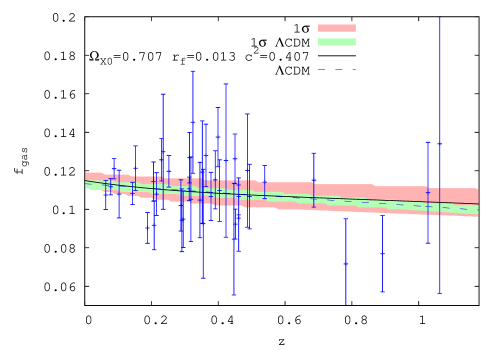
Figure 5: Gas mass fraction in 42 relaxed galaxy clusters vs. redshift. The solid and dashed curves correspond to the best fit models: holographic and $\Lambda$CDM, respectively. The data points with their error bars are taken from Table III of Ref. Allen .

IV.5 History of the Hubble parameter

Recently, high precision measurements by Riess et al. at $z=0$, from the observation of 240 Cepheid variables of rather similar periods and metallicities Riess-2009 , as well as measurements by Gaztañaga et al., at $z=0.24,\,0.34,{\rm and}\,0.43\,$ gazta , who used the BAO peak position as a standard ruler in the radial direction, have somewhat improved our knowledge about $H(z)$. However, at redshifts above, say, $0.5$ this function remains largely unconstrained. Yet, in order to constrain the holographic model we have employed these four data alongside 11 noisier data in the redshift interval $0.1\lesssim z\lesssim 1.8$, from Simon et al. simon and Stern et al. stern , obtained from the differential ages of passive-evolving galaxies and archival data.

By minimizing

$$\chi^{2}_{Hubble}({\bf p})=\sum_{i=1}^{15}\frac{[H_{th}(z_{i})\,-\,H_{obs}(z_{i})]^{2}}{\sigma^{2}(z_{i})}$$ (35)

we got $\chi^{2\,(minimum)}_{Hubble}=9.57$ and $H_{0}=71.8\pm 2.9\,$ km/s/Mpc as the best fit for the Hubble’s constant. Figure 6 depicts the Hubble history according to the best fit holographic model and the best $\Lambda$CDM model.

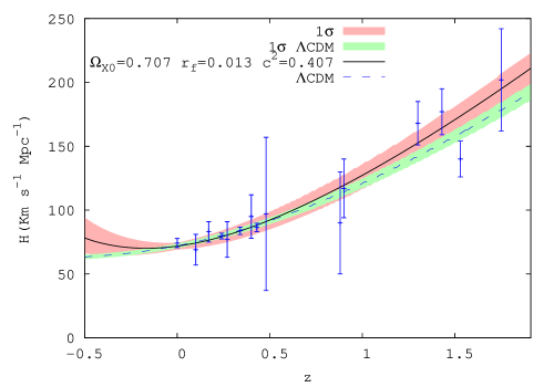
Figure 6: History of the Hubble factor in terms of the redshift for the best fit values of the holographic model (solid line) and the $\Lambda$CDM model (dashed line). The data points and error bars are borrowed from Refs. Riess-2009 ; gazta ; simon ; stern .

IV.6 Growth function

Up to now, we have considered background quantities that chiefly depend on $H(z)$ whence they are not very useful at discriminating between cosmological models that present a similar Hubble history, independently of how different they are otherwise. One manner to circumvent this hurdle is to study evolution of the growth function $f=d\ln\delta_{M}/d\ln a$, where $\delta_{M}$ denotes the density contrast of non-relativistic matter.

The evolution of the latter obeys the coupled set of equations

$$\dot{\delta}_{M}-\frac{k^{2}}{a}v_{M}=-\frac{1+r}{r}Q\,H\,\delta_{M}\,,$$ (36)

$$\dot{v}_{M}+Hv_{M}+\frac{1}{a}\phi=0\,,$$ (37)

where the Newtonian potential $\phi$ fulfills Poisson’s equation

$$\frac{k^{2}}{a^{2}}=-4\pi G\rho_{M}\delta_{M}\,.$$ (38)

Solving the equations, and expressing in terms of $r$ and using $w=[c^{2}(1\,+\,r)\,-\,2]/(3c^{2})$ obtained from (4), $c^{-2}(1\,+\,r)^{-1}=(\dot{H}/H^{2})\,+\,2$, and (11), we get from the evolution equations (9) and (10)

$$f^{\prime}+f^{2}+\left(\frac{1}{c^{2}(1+r)}+Q\frac{1+r}{r}\right)f-\frac{3r^{3}+2Q^{2}(1+r)^{3}-2Qr(2+r-r^{2})}{2r^{2}(1+r)}=0\,,$$ (39)

where $f^{\prime}\equiv df/d\ln a$. Note that in the limit $Q\rightarrow 0$, last equation collapses to the corresponding expression of the Einstein-de Sitter scenario ($\Omega_{M}(z)=1$ and $\delta_{M}\propto a\propto t^{2/3}$); that is to say, $f^{\prime}+f^{2}+[2\,+\,(\dot{H}/H^{2})]f=3\Omega_{M}/2$. (Recall that in Einstein-de Sitter $\dot{H}/H^{2}=-3/2$ and the solution of the equation for $f$ is simply $f=1$).

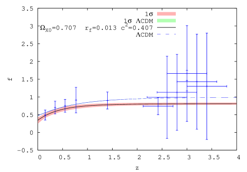
Figure 7: Growth function, $f$, vs. redshift as follows from integrating Eq. (39)(solid line). Also shown is the prediction of the $\Lambda$CDM model (dashed line). The observational data were taken from Ref. Gong . In constraining both models we have used only the five less noisy data depicted in the figure, (i.e., data corresponding to redshifts below $1.5$).

In constraining the model we have taken only the five lowest redshift data of the growth function shown in Fig. 7 -the other data present very large error bars. The best fit yields $\chi^{2}=1.06$.

Figures 8 - 10 and table I summarize our findings.

Figure 10 depicts the $1\sigma$ confidence contours from SN Ia (dashed yellow), CMB-shift (solid black), BAO (dashed blue), x-rays (dashed black), history of the Hubble function (dot-dot dashed green), and grow function (dot-dashed red) in the ($\Omega_{X0},c^{2}$) plane (left panel) and the ($\Omega_{X0},r_{f}$) plane. The joined constraints corresponding to $\chi^{2}_{total}$ are shown as shaded contours. As is apparent from left panel most of the discriminatory power arises from the near orthogonality between the x-ray and CMB-shift and supernovae contours. However, in the right panel the supernovae contour appears nearly degenerated with respect to the x-ray contour.

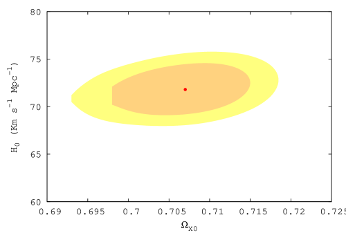
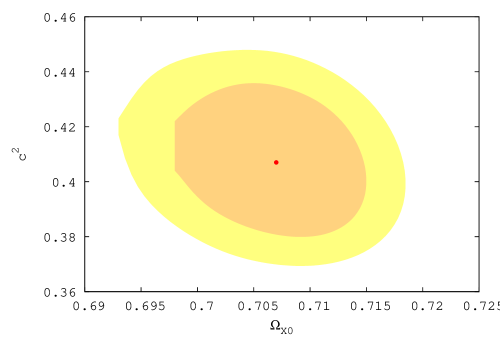
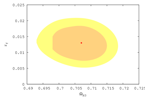
Figure 8: Panels from left to right show the 68.3% and 95.4% confidence contours for the pair of free parameters ($\Omega_{X0}$, $H_{0}$), ($\Omega_{X0}$, $c^{2}$), ($\Omega_{X0}$, $r_{f}$), respectively, obtained by constraining the holographic model with SN Ia+CMB-shift+ BAO+x-ray+H(z)+growth function data. The solid point in each panel locates the best fit values.

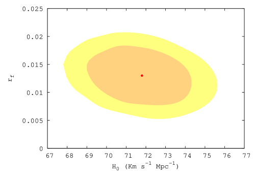
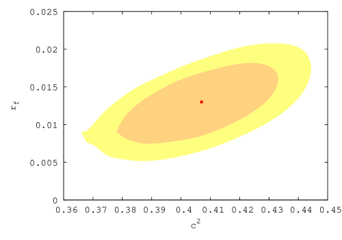
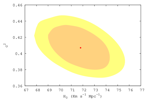
Figure 9: Same as Fig. 8 for the pairs of free parameters ($H_{0}$, $r_{f}$), ($c^{2}$, $r_{f}$), and ($H_{0}$, $c^{2}$).

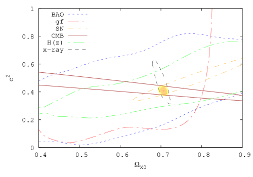
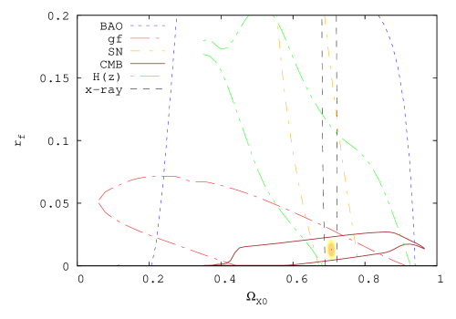
Figure 10: Left panel: The probability contours for SN Ia, CMB, BAO, x-ray, $H(z)$, and growth function, in the ($\Omega_{X0},c^{2}$) plane. The joined constraint uses $\chi^{2}_{\rm total}=\chi^{2}_{sn}\,+\,\chi^{2}_{cmb}\,+\,\chi^{2}_{bao}\,+\,\chi^{2}_{x-rays}+\,\chi^{2}_{Hubble}\,+\,\chi^{2}_{gf}$. Right panel: Idem for the ($\Omega_{X0},r_{f}$) plane.

Altogether, by constraining the holographic model of Section II with data from SN Ia, CMB-shif, BAO, x-rays, H(z), and the growth function we obtain $\Omega_{X0}=0.707\pm 0.009$, $c^{2}=0.407^{+0.033}_{-0.028}$, $r_{f}=0.013^{+0.006}_{-0.005}$, and $H_{0}=71.8\pm 2.9$ km/s/Mpc as best fit parameters. It is worth noticing that the non-interacting case, $Q=0$ (which implies $r_{f}=0$ via Eq. (12)), lies over $2\sigma$ away from the best fit value. This feature seems typical of holographic dark energy models (see e.g. gao ; suwa ; id-jcap ).

Table 1 shows the partial, total, and total $\chi^{2}$ over the number of degrees of freedom of the holographic model along with the corresponding values for the $\Lambda$CDM model. In the latter one has just two free parameters, $\Omega_{M0}$ and $H_{0}$. Their best fit values after constraining the model to the data are $\Omega_{M0}=0.266\pm 0.006$, and $H_{0}=71.8\pm 1.9\,$km/s/Mpc.

Model	$\chi^{2}_{sn}$	$\chi^{2}_{cmb}$	$\chi^{2}_{bao}$	$\chi^{2}_{x-rays}$	$\chi^{2}_{H}$	$\chi^{2}_{gf}$	$\chi^{2}_{{\rm total}}$	$\chi^{2}_{{\rm total}}/dof$
Holographic	$543.70$	$0.01$	$1.20$	$41.79$	$9.57$	1.06	$597.34$	$\;\;0.96$
$\Lambda$CDM	$542.87$	$0.05$	$1.13$	$41.59$	$8.73$	0.43	$594.80$	$\;\;0.96$

Table 1: $\chi^{2}$ values of the best fit holographic model ($\Omega_{X}=0.707\pm 0.009$, $\;c^{2}=0.407^{+0.033}_{-0.028}$,$\;r_{f}=0.013^{+0.006}_{-0.005}$, and $H_{0}=71.8\pm 2.9\,$km/s/Mpc), and the best fit $\Lambda$CDM model ($\Omega_{M0}=0.266\pm 0.006$, and $H_{0}=71.8\pm 1.9\,$ km/s/Mpc).

Although the $\Lambda$CDM model fits the data somewhat better, $\Delta\chi^{2}\simeq 2.5$, than the holographic model, that has two more free parameters, it its uncertain which model should be preferred in view that the former cannot address the cosmic coincidence problem and the latter substantially alleviates it. More abundant and accurate data, especially at redshifts between the supernovae range and the CMB, will help decide the issue. Nonetheless, we believe that the uncertainty will likely persists till a breakthrough on the theoretical side allows us to calculate with confidence the true value of the cosmological constant.

V Concluding remarks

We performed a statistical study of the best fit parameters of the holographic model -presented in section II- using data from SN Ia, CMB-shift, BAO, x-ray, the Hubble history, and the growth function; 621 data in total. The maximum likelihood (or minimum $\chi^{2}$) parameters are $\Omega_{X0}=0.707\pm 0.009$, $c^{2}=0.407^{+0.033}_{-0.028}$, $r_{f}=0.013^{+0.006}_{-0.005}$, and $H_{0}=71.8\pm 2.9$ km/s/Mpc with $\chi^{2}/dof\approx 0.96$. The $\Omega_{X0}$ and $H_{0}$ values fall within $1\sigma$ of the corresponding values determined by Komatsu et al. komatsu ($0.734\pm 0.029$ and $71.0\pm 2.5$ km/s/Mpc, respectively). The evolution of the equation of state parameter, $w$, at redshift below $1.2$ (see right panel of Fig. 2) is compatible with the observational constraints derived in serra-prd and, as in other Ricci’s holographic models gao ; lxu ; suwa ; lepe , it crosses the phantom divide line at recent times (see right panel of Fig. 2). Curiously enough, the $\Omega_{X0}$ and $c^{2}$ best fit values of this model agree within $1\sigma$ with the corresponding values obtained by Suwa et al. suwa despite the use of a very different interaction term between the dark components.

It is to be emphasized that holographic models do not contain the $\Lambda$CDM model as a limiting case since the energy density of the quantum vacuum, being constant, cannot be holographic. It is also noteworthy that, in general, the $c^{2}$ term in the holographic expression for the dark energy, Eq. (1), should not be considered constant except precisely when the Ricci’s length is chosen as the infrared cutoff nd-jcap .

A lingering problem, both for this model and the $\Lambda$CDM model, refers to the age of the old quasar APM 08279+5255 at redshift $z=3.91$. In both models the measured quasar age would fall within $1\sigma$ only if the Hubble constant, $H_{0}$, would come down substantially -something we do not expect though it cannot be excluded. Accordingly, we must wait for further observational data to see whether the present tension gets exacerbated or disappears.

Before closing, it results interesting to contrast the model explored in this paper with the model of Ref. id-jcap . The present one shows a better fit to the growth function at low redshifts, as well as to the CMB-shift and BAO data. However, it does not fit so well the age of the old quasar APM 08279+5255.

- (1) J.A. Friemann, M.S. Turner and D. Huterer, Ann. Rev. Astron. Astrophys. 46, 385 (2008); R. Durrer and R. Maartens, Gen. Relativ. Grav. 40, 301; L. Amendola and Tsujikawa, Dark Energy. Theory and Observations (CUP, Cambridge, 2010).
- (2) G. ’t Hooft, “Dimensional reduction in quantum gravity”, preprint gr-qc/9310026; L. Susskind, J. Math. Phys. (N.Y.) 36, 6377 (1995).
- (3) A. G. Cohen, D.B. Kaplan and A.E. Nelson, Phys. Rev. Lett. 82, 4971 (1999); M. Li, Phys. Lett. B 603, 1 (2004).
- (4) Y.J. Ng, Phys. Rev. Lett. 86, 2946 (2001); M. Arzano, T.W. Kephart, and Y.J. Ng, Phys. Lett. B 649, 243 (2007).
- (5) W. Zimdahl and D. Pavón, Class. Quantum Grav. 24, 5461 (2007).
- (6) S. D. H. Hsu, Phys. Lett. B 594, 13 (2004); D. Pavón and W. Zimdahl, Phys. Lett. B 628, 206 (2005); B. Guberina, R. Horvat, and H. Nikolic, JCAP01 (2007) 012; L. Xu, JCAP09 (2009) 016.
- (7) C. Gao, F. Wu, X. Chen, and Y.G. Shen, Phys. Rev. D 79, 043511 (2009).
- (8) L. Xu, W. Li, and J. Lu, Mod. Phys. Lett. A 24, 1355 (2009).
- (9) M. Suwa, T. Nihei, Phys. Rev. D 81, 023519 (2010).
- (10) S. Lepe and F. Pena, European Physical Journal (in the press), arXiv:10052.2180 [hepth].
- (11) R. Brustein, “Cosmological entropy bounds”, in String Theories and Fundamental Interactions, Lecture Notes Physics 737, 619 (2008), hep-th/0702108.
- (12) L. Amendola, Phys. Rev. D 62, 043511 (2000); D. Tocchini-Valentini and L. Amendola, Phys. Rev. D, 65 063508 (2002).
- (13) S. del Campo, R. Herrera, and D. Pavón, Phys. Rev. D 78, 021302(R) (2008); ibid. JCAP01 (2009) 020.
- (14) E. Abdalla, L.R. Abramo, and J.C.C. Souza, Phys. Rev. D 82, 023508 (2010).
- (15) J. Lee, Astrophys. J. Letters (in the press), arXiv:1008.4620 [astro-ph.CO].
- (16) C. Wetterich, Nucl. Phys. B, 302, 668 (1988);ibid Astron. Astrophys. 301, 321 (1995).
- (17) Jerôme Martin, personal communication.
- (18) L.P. Chimento, A.S. Jakubi, and D. Pavón, Phys. Rev. D 67, 087302 (2003).
- (19) L.P. Chimento, A.S. Jakubi, D. Pavón, and W. Zimdahl, Phys. Rev. D., Phys. Rev. D 67, 083513 (2003); G. Olivares, F. Atrio-Barandela, and D. Pavón, Phys. Rev. D 71, 063523 (2005).
- (20) D. Pavón and B. Wang, Gen. Relativ. Grav. 41, 1 (2009).
- (21) P. Serra et al., Phys. Rev. D 80, 121302 (2009).
- (22) R.A. Daly, S.G. Djorgovski, K.A. Freeman, M. Mory, C.P. O’Dea, P. Kharb, and S. Baum, Astrophys. J. 677, 1 (2008).
- (23) I. Durán, D. Pavón, and W. Zimdahl, JCAP07 (2010) 018.
- (24) A.C.S. Friaça, J.S. Alcaniz, and J.A.S. Lima, Mon. Not. R. Astron. Soc. 362, 1295 (2005).
- (25) J. Dunlop et al., “Old Stellar Populations in Distant Radio Galaxies”, in The Most Distant Radio Galaxies, eds. H.J.A. Rottgering, P. Best and M.D. Lehnert (Kluwer, Dordrecht, 1999), p. 71.
- (26) J. Dunlop et al., Nature (London) 381, 581 (1996).
- (27) H. Spinrad et al., Astrophys. J. 484, 581 (1997).
- (28) G. Hasinger et al., Astrophys. J. 573, L77 (2002); S. Komossa and G. Hasinger, in Proc. of the Workshop “XEUS -Studying the Evolution of the Hot Universe”, eds. G. Hasinger et al., astro-ph/0207321.
- (29) R. Amanullah et al. (The Supernova Cosmology Project), Astrophys. J. (in the press), arXiv:1004.1711.
- (30) S. Nesseris and L. Perivolaropoulos, Phys. Rev. D 72, 123519 (2005).
- (31) Y. Wang and P. Mukherjee, Astrophys. J. 650, 1 (2006).
- (32) J.R. Bond, G. Efstathiou, and M. Tegmark, Mon. Not. R. Astron. Soc. 291, L33 (1997).
- (33) E. Komatsu et al., Astrophys. J. Suppl. 180, 330 (2009).
- (34) D.J. Eisenstein et al. [DSS Collaboration] Astrophys. J. 633, 560 (2005).
- (35) W.J. Percival et al., Mon. Not. R. Astron. Soc. 401, 2148 (2010).
- (36) S. Nesseris and L. Perivolaropoulos, JCAP01 (2007) 018.
- (37) S.M.D. White, J. F. Navarro, A. Evrard, and C.S. Frenk, Nature 366, 429 (1993).
- (38) S.W. Allen et al., Mon. Not. R. Astron. Soc. 383, 879 (2008).
- (39) A.G. Riess, et al., Astrophys. J. 699, 539 (2009).
- (40) E. Gaztañaga, A. Cabré, and L. Hui, Mon. Not. R. Astron. Soc. 399, 1663 (2009).
- (41) J. Simon, L. Verde, and R. Jiménez, Phys. Rev. D 71, 123001 (2005).
- (42) D. Stern, R. Jiménez, L. Verde, M. Kamionkowski, and S.A. Stanford, JCAP02 (2010) 008.
- (43) Y. Gong, Phys. Rev. D 78, 123010 (2008).
- (44) N. Radicella and D. Pavón, JCAP10 (2010) 005.