Renormalization constants for one-derivative
       fermion operators in twisted mass QCD

Abstract:

We present perturbative and non-perturbative results on the renormalization constants of the local and one-derivative vector and axial vector operators. Non-perturbative results are obtained using the twisted mass Wilson fermion formulation employing two degenerate dynamical quarks and the tree-level Symanzik improved gluon action for pion masses in the range of about 450-260 MeV and at there values of the lattice spacing, namely 0.055 fm, 0.070 fm and 0.089 fm. Subtraction of ${\cal O}(a^{2})$ terms is carried out by performing the perturbative evaluation of these operators at 1-loop and up to ${\cal O}(a^{2})$. The renormalization conditions are defined in the RI^′-MOM scheme, for both perturbative and non-perturbative results. The Z-factors, obtained for different values of the renormalization scale, are evolved perturbatively to a reference scale set by the inverse of the lattice spacing. In addition, they are translated to $\overline{MS}$ at 2 GeV using 3-loop perturbative results for the conversion factors.

1 Introduction

Simulations in lattice QCD have advanced remarkably in the past couple of years reaching the physical pion mass. The theoretical and algorithmic improvements, combined with the tremendous increase in computational power, have made ab initio calculations of key observables on hadron structure in the chiral regime feasible enabling comparison with experiment. Form factors and generalized parton distribution functions (GPDs) can be obtained from the generalized form factors in certain limiting cases. GPDs provide detailed information on the internal structure of hadrons in terms of both the longitudinal momentum fraction and the total momentum transfer squared. Beyond the information that the form factors yield, such as size, magnetization and shape, GPDs encode additional information, relevant for experimental investigations, such as the decomposition of the total hadron spin into angular momentum and spin carried by quarks and gluons. GPDs are single particle matrix elements of the light-cone operator [1, 2], which can be expanded in terms of local twist-two operators ${\cal O}_{\Gamma}^{f,\{\mu_{1}\mu_{2}\cdots\mu_{n}\}}=\overline{\psi}^{f}\Gamma^{\{\mu_{1}}i\buildrel\leftrightarrow\over{D}\raise-1.0pt\hbox{}^{\mu_{2}}\cdots i\buildrel\leftrightarrow\over{D}\raise-1.0pt\hbox{}^{\mu_{n}\}}\psi^{f}$. Lattice QCD allows us to extract hadron matrix elements for the twist-2 operators, which can be expressed in terms of generalized form factors.

In order to compare hadron matrix elements of these local operators to experiment one needs to renormalize them. The aim of this paper is to calculate non-perturbatively the renormalization factors of the above twist-two fermion operators within the twisted mass formulation. We show that, although the lattice spacings considered in this work are smaller than $1$ fm, ${\cal O}(a^{2})$ terms are non-negligible and introduce significantly larger uncairtainties than statistical errors. We therefore compute the ${\cal O}(a^{2})$ terms perturbatively and subtract them from the non-perturbative results. This subtraction suppresses lattice artifacts considerably depending on the operator under study and leads to a more accurate determination of the renormalization constants [3, 4].

2 Formulation

For the gauge fields we use the tree-level Symanzik improved gauge action [5], which includes besides the plaquette term also rectangular $(1\times 2)$ Wilson loops. The fermionic action for two degenerate flavors of quarks in twisted mass QCD is given by

$$S_{F}=a^{4}\sum_{x}\overline{\chi}(x)\bigl{(}D_{W}[U]+m_{0}+i\mu_{0}\gamma_{5}\tau^{3}\bigr{)}\chi(x)$$ (1)

with $\tau^{3}$ the Pauli matrix, $\mu_{0}$ the bare twisted mass and $D_{W}$ the massless Wilson-Dirac operator. Maximally twisted Wilson quarks are obtained by setting the untwisted bare quark mass $m_{0}$ to its critical value $m_{\rm cr}$, while the twisted quark mass parameter $\mu_{0}$ is kept non-vanishing in order to give the light quarks their mass. In $\rm Eq.~{}(\ref{action})$ the quark fields $\chi$ are in the so-called “twisted basis”. The “physical basis” is obtained for maximal twist by the simple transformations $\psi(x)=\exp\left(\frac{i\pi}{4}\gamma_{5}\tau^{3}\right)\chi(x),\,\,\overline{\psi}(x)=\overline{\chi}(x)\exp\left(\frac{i\pi}{4}\gamma_{5}\tau^{3}\right)$.

Here we consider only the vector and axial twist-two operators up to one-derivative, $Z_{\rm V}$, $Z_{\rm A}$, $Z_{\rm DV}$, $Z_{\rm DA}$ (symmetrized over two Lorentz indices and traceless), which are given in the twisted basis as follows:

$$\mathcal{O}_{V}^{a} =\bar{\chi}\gamma_{\mu}\tau^{a}\chi =\begin{cases}\bar{\psi}\gamma_{5}\gamma_{\mu}\tau^{2}\psi&a=1\\ -\bar{\psi}\gamma_{5}\gamma_{\mu}\tau^{1}\psi&a=2\\ \bar{\psi}\gamma_{\mu}\tau^{3}\psi&a=3\end{cases}$$

$$\mathcal{O}_{A}^{a} =\bar{\chi}\gamma_{5}\gamma_{\mu}\tau^{a}\chi =\begin{cases}\bar{\psi}\gamma_{\mu}\tau^{2}\psi&a=1\\ -\bar{\psi}\gamma_{\mu}\tau^{1}\psi&a=2\\ \bar{\psi}\gamma_{5}\gamma_{\mu}\tau^{3}\psi&a=3\end{cases}$$

$$\mathcal{O}_{\rm DV}^{\{\mu\,\nu\}\,a} =\overline{\chi}\gamma_{\{\mu}\overleftrightarrow{D}_{\nu\}}\tau^{a}\chi =\begin{cases}\overline{\psi}\gamma_{5}\gamma_{\{\mu}\overleftrightarrow{D}_{\nu\}}\tau^{2}\psi&a=1\\ -\overline{\psi}\gamma_{5}\gamma_{\{\mu}\overleftrightarrow{D}_{\nu\}}\tau^{1}\psi&a=2\\ \overline{\psi}\gamma_{\{\mu}\overleftrightarrow{D}_{\nu\}}\tau^{3}\psi&a=3\end{cases}$$

$$\mathcal{O}_{\rm DA}^{\{\mu\,\nu\}\,a} =\overline{\chi}\gamma_{5}\gamma_{\{\mu}\overleftrightarrow{D}_{\nu\}}\tau^{a}\chi =\begin{cases}\overline{\psi}\gamma_{\{\mu}\overleftrightarrow{D}_{\nu\}}\tau^{2}\psi&\quad a=1\\ -\overline{\psi}\gamma_{\{\mu}\overleftrightarrow{D}_{\nu\}}\tau^{1}\psi&\quad a=2\\ \overline{\psi}\gamma_{5}\gamma_{\{\mu}\overleftrightarrow{D}_{\nu\}}\tau^{3}\psi&\quad a=3\end{cases}$$ (2)

In a massless renormalization scheme the renormalization constants are defined in the chiral limit, where isospin symmetry is exact. Hence, the same value for $Z$ is obtained independently of the value of the isospin index $a$ and therefore we drop the $a$ index from here on. However, one must note that, for instance, the physical $\overline{\psi}\gamma_{\{\mu}\overleftrightarrow{D}_{\nu\}}\tau^{1}\psi$ is renormalized with $Z_{\rm DA}$, while $\overline{\psi}\gamma_{\{\mu}\overleftrightarrow{D}_{\nu\}}\tau^{3}\psi$ requires the $Z_{\rm DV}$, which differ from each other even in the chiral limit. The one-derivative operators fall into different irreducible representations of the hypercubic group, depending on the choice of indices. Hence, we distinguish between $\mathcal{O}_{\rm DV1}\,(\mathcal{O}_{\rm DA1})=\mathcal{O}_{\rm DV}\,\,(\mathcal{O}_{\rm DA})$ with $\mu=\nu$ and $\mathcal{O}_{\rm DV2}\,(\mathcal{O}_{\rm DA2})=\mathcal{O}_{\rm DV}\,(\mathcal{O}_{\rm DA})$ with $\mu\neq\nu$.

2.1 Renormalization Condition

The renormalization constants are computed both perturbatively and non-perturbatively in the RI^′-MOM scheme at various renormalization scales. We translate them to the ${\overline{\rm MS}}$-scheme at (2 GeV)² using a conversion factor computed in perturbation theory to ${\cal O}(g^{6})$ as described in Section 3. The Z-factors are determined by imposing the following conditions:

$$Z_{q}=\frac{1}{12}{\rm Tr}\left[\frac{-i\sum_{\rho}\gamma_{\rho}p_{\rho}}{p^{2}}\,(S^{L}(p))^{-1}\right]\Bigr{|}_{p^{2}=\mu^{2}}\,,\quad Z_{q}^{-1}\,Z^{\mu\nu}_{\cal O}\,\frac{1}{12}{\rm Tr}\left[(-i\,{\cal\tilde{O}}_{\{\mu}\,\,p_{\nu\}})^{-1}\,\Gamma^{L}_{\mu\nu}(p)\right]\Bigr{|}_{p^{2}=\mu^{2}}=1\,,$$ (3)

where $\mu$ is the renormalization scale, $S_{L}$ and $\Gamma_{L}$ correspond to the perturbative or non-perturbative results and ${\cal\tilde{O}}_{\{\mu}\,\,p_{\nu\}}$ is the tree-level expression of the operator under study. The trace is taken over spin and color indices, and the conditions are imposed in the massless theory.

2.2 Perturbative procedure

Our calculation for the Z-factors is performed in 1-loop perturbation theory to ${\cal O}(a^{2})$. The order $a^{2}$-terms can be subtracted from non-perturbative estimates, and they can eliminate possible large lattice artifacts. There are many difficulties when extracting powers of the lattice spacing from our expressions, since there appear singularities encountered at ${\cal O}(a^{2})$, that persist even up to 6 dimensions (integral convergence in 7-d), making their extraction more delicate. In addition to that, there appear Lorentz non-invariant contributions in ${\cal O}(a^{2})$-terms, such as $\sum_{\mu}p_{\mu}^{4}/p^{2}$, where $p$ is the external momentum; as a consequence, the Z-factors also depend on such terms.

For all our perturbative results we employ a Wilson-type fermion action (Wilson/clover/twisted mass), with non-zero bare mass, $m$. For the renormalization of the fermion field and the local bilinears we also have a finite twisted mass parameter, $\mu_{0}$, so we can explore the mass dependence. For gluons we use Symanzik improved actions (Plaquette, Tree-level Symanzik, Iwasaki, TILW, DBW2) [6]. The expressions for the matrix elements and the Z-factors are given in a general covariant gauge, and their dependence on the coupling constant, the external momentum, the masses and the clover parameter $\,c_{\rm SW}$ is shown explicitly. The Feynman diagrams involved in the computation of the various Z-factors are illustrated in Fig. 1.

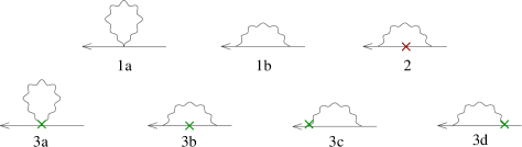
Figure 1: One-loop diagrams contributing to the correction of the amputated Green’s functions of the propagator (1a, 1b), local bilinears (2) and one-derivative operators (3a-3d). A wavy (solid) line represents gluons (fermions). A cross denotes an insertion of the operator under study.

Here we do not show any expressions for the matrix elements of the Green’s functions, since they are far too lengthy. As an example we show the ${\cal O}(a^{2})$ terms that can improve the non-perturbative estimate of $Z_{q}$ once they are subtracted. For the special choices: $c_{SW}=0$, $r=1$ (Wilson parameter), $\lambda=0$ (Landau gauge), $m_{0}=0$, $\mu_{0}=0$, and for tree-level Symanzik gluons, $Z_{q}$ can be corrected to ${\cal O}(a^{2})$ as follows:

$$Z_{q}^{\rm impr}=Z_{q}^{\rm non-pert}-\frac{{a^{2}}g^{2}C_{F}}{16\pi^{2}}\Big{[}\mu^{2}\big{(}1.1472{-}\frac{73}{360}\ln({a^{2}}\mu^{2})\big{)}{+}\frac{\sum_{\rho}\mu_{\rho}^{4}}{\mu^{2}}\big{(}2.1065{-}\frac{157}{180}\ln({a^{2}}\mu^{2})\big{)}\Bigr{]}$$ (4)

Its most general expression is far too lengthy to be included in paper form; it is provided, along with the rest of our results for the Z-factors, in electronic form in Ref. [4].

2.3 Non-perturbative calculation

For each operator we define a bare vertex function given by

$$G(p)=\frac{a^{12}}{V}\sum_{x,y,z,z^{\prime}}e^{-ip(x-y)}\langle u(x)\overline{u}(z)\mathcal{J}(z,z^{\prime})d(z^{\prime})\overline{d}(y)\rangle\,,\vspace{-0.15cm}$$ (5)

where $p$ is a momentum allowed by the boundary conditions, $V$ is the lattice volume, and the gauge average is performed over gauge-fixed configurations. The form of $\mathcal{J}(z,z^{\prime})$ depends on the operator under study, for example $\mathcal{J}(z,z^{\prime}){=}\delta_{z,z^{\prime}}\gamma_{\mu}$ would correspond to the local vector current. In the literature there are two main approaches that have been employed for the evaluation of Eq. (5). The first approach relies on translation invariance to shift the coordinates of the correlators in Eq. (5) to position $z{=}0$ [7]. Having shifted to $z{=}0$ allows one to calculate the amputated vertex function for a given operator $\mathcal{J}$ for any momentum with one inversion per quark flavor. In this work we explore the second approach, introduced in Ref. [8], which uses directly Eq. (5) without employing translation invariance. One must now use a source that is momentum dependent but can couple to any operator. For twisted mass fermions, with twelve inversions one can extract the vertex function for a single momentum. The advantage of this approach is a high statistical accuracy and the evaluation of the vertex for any operator including extended operators at no significant additional computational cost. We fix to Landau gauge using a stochastic over-relaxation algorithm [9].

3 Results

We perform the non-perturbative calculation of renormalization constants for three values of the lattice spacing, $a$=0.089 fm, 0.070 fm, 0.056 fm, corresponding to $\beta=3.9,\,4.05$ and $4.20$ respectively. In Tables I and II of Ref. [3] we summarize the various parameters that we used in our simulations. We have tested finite volume effects and pion mass dependence; both effects are within the small statistical errors for the operators considered here. Chiral extrapolations are necessary to obtain the renormalization factors in the chiral limit. Since the dependence on the pion mass is insignificant, even if we allow a slope and perform a linear extrapolation to our data, this is consistent with zero; therefore the renormalization constants are computed at one quark mass. Figures 2-3 demonstrate the effect of subtraction at two $\beta$ values for the local and one-derivative vector/axial Z-factors, as a function of the renormalization scale (in lattice units). $Z_{\rm V}$ and $Z_{\rm A}$ are scale independent, thus we obtain a very good plateau upon subtraction of ${\cal O}(a^{2})$ effects. To identify a plateau for $Z_{\rm DV}$ and $Z_{\rm DA}$ we need to convert to $\overline{\rm MS}$ and evolve to a reference scale.

      

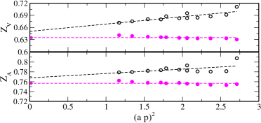
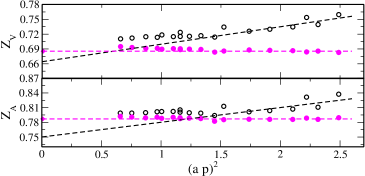
Figure 2: Renormalization scale dependence for $Z_{\rm V}$, $Z_{\rm A}$ at $\beta=3.9,\,m_{\pi}=0.430$ GeV (left panel) and $\beta=4.20,\,m_{\pi}=0.476$ GeV (right panel) (Open points: unsubtracted, filled points: subtracted).

   

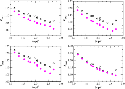
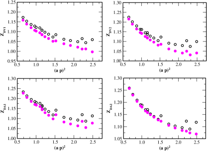
Figure 3: Renormalization scale dependence for $Z_{\rm DV}$, $Z_{\rm DA}$ (RI^′-MOM scheme before evolving at a reference scale) at $\beta=3.9,\,m_{\pi}=0.430$ GeV (left panel) and $\beta=4.20,\,m_{\pi}=0.476$ GeV (right panel) (Open points: unsubtracted, filled points: subtracted).

$\bullet$ Conversion to ${\overline{\rm MS}}$: The passage to the continuum ${\overline{\rm MS}}$-scheme is accomplished through use of a conversion factor, which is computed up to 3 loops in perturbation theory. By definition, this conversion factor is the same for the one-derivative vector and axial renormalization constant, but will differ for the cases $Z_{\rm DV1}\,(Z_{\rm DA1})$ and $Z_{\rm DV2}\,(Z_{\rm DA2})$, that is $C_{\rm DV1}\equiv C_{\rm DA1}=Z^{\overline{\rm MS}}_{\rm DV}/Z^{\rm RI^{\prime}}_{\rm DV1},\,C_{\rm DV2}\equiv C_{\rm DA2}=Z^{\overline{\rm MS}}_{\rm DV}/Z^{\rm RI^{\prime}}_{\rm DV2}$. This requirement for different conversion factors results from the fact that the Z-factors in the continuum ${\overline{\rm MS}}$-scheme do not depend on the external indices, $\mu,\,\nu$ (see Eq. (2.5) of Ref. [10]), while the results in the RI^′-MOM scheme do depend on $\mu$ and $\nu$. We also need another factor $R(2GeV,\mu)$ that will bring all Z-factors down to $\mu=2$ GeV, for example

$$Z^{\overline{\rm MS}}_{\rm DV1}(2GeV)=R_{\rm DV}(2GeV,\mu)\cdot C_{\rm DV1}(\mu)\cdot Z^{\rm RI^{\prime}}_{\rm DV1}(\mu)$$ (6)

      

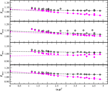
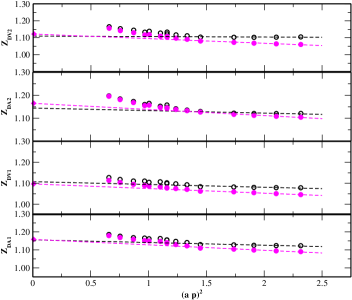
Figure 4: Renormalization factors at $\beta=3.9,\,m_{\pi}=0.430$ GeV (left panel) and $\beta=4.20,\,m_{\pi}=0.476$ GeV (right panel) in the ${\overline{\rm MS}}$-scheme at 2 GeV. The lines show extrapolations to $a^{2}p^{2}=0$ within the range $p^{2}\sim 15-32$ (GeV)². (Open points: unsubtracted, filled points: subtracted)

A “renormalization window” should exist for $\Lambda_{QCD}^{2}<<\mu^{2}<<1/a^{2}$ where perturbation theory holds and finite-$a$ artifacts are small, leading to scale-independent results (plateau). In practice such a condition is hard to satisfy: The upper range of the inequality is extended to $(2-5)/a^{2}$ leading to lattice artifacts in our results that are of ${\cal O}(a^{2}p^{2})$. Fortunately our perturbative calculations allow us to subtract the leading perturbative $O(a^{2})$ lattice artifacts which alleviates the problem. To remove the remaining $O(a^{2}p^{2})$ artifacts we extrapolate linearly to $a^{2}p^{2}=0$ as demonstrated in Fig. 4. The statistical errors are negligible and therefore an estimate of the systematic errors is important. We note that, in general, the evaluation of systematic errors is difficult. The largest systematic error comes from the choice of the momentum range to use for the extrapolation to $a^{2}p^{2}=0$. One way to estimate this systematic error is to vary the momentum range where we perform the fit. Another approach is to fix a range and then eliminate a given momentum in the fit range and refit. The spread of the results about the mean gives an estimate of the systematic error. In the final results we give as systematic error the largest one from using these two procedures which is the one obtained by modifying the fit range. In order to treat all beta values equally, we fix the momentum range in physical units and we thus fit all renormalization constants in the same physical momentum range, $p^{2}\sim 15-32$ (GeV)². The momentum interval in physical units has bean chosen such as a good plateau exists at each $\beta$, as can be seen in Fig. 4. The ${\cal O}(a^{2})$ perturbative terms which we subtract, decrease as $\beta$ increases, as expected. The momentum range in lattice units at each $\beta$ is rescaled as follows: $\beta=3.9:a^{2}p^{2}\sim 3-5$, $\beta=4.05:a^{2}p^{2}\sim 1.9-3$, $\beta=4.20:a^{2}p^{2}\sim 1.2-2.5$. Our results for the ${\cal O}(a^{2})$ corrected $Z$-factors in the $\overline{\rm MS}$-scheme at 2 GeV are given in Table 1, which have been obtained by extrapolating linearly in $a^{2}p^{2}$. For $Z_{\rm DV}$ and $Z_{\rm DA}$ we used the fixed momentum range $p^{2}\sim 15-32$ (GeV)² [3], while for $Z_{\rm V}$ and $Z_{\rm A}$ we used all the data points available, since the plateau is good for all momenta. The final results for $Z_{\rm V}$ and $Z_{\rm A}$ for a more extended momentum range will appear in [4].

$\beta$	$\,\,Z_{\rm V}\,\,$		$\,\,Z_{\rm A}\,\,$		$\,\,Z_{\rm DV1}\,\,$		$\,\,Z_{\rm DV2}\,\,$		$\,\,Z_{\rm DA1}\,\,$		$\,\,Z_{\rm DA2}\,\,$
3.90	$\,\,0$.	6343(6)(3)	$\,\,0$.	7561(6)(5)		0.970(34)(26)		1.061(23)(29)		1.126(22)(78)		1.076(5)(1)
4.05	$\,\,0$.	6628(7)(14)	$\,\,0$.	7722(6)(3)		1.033(11)(14)		1.131(23)(18)		1.157(9)(7)		1.136(5)
4.20	$\,\,0$.	6854(5)(13)	$\,\,0$.	7870(5)(9)		1.097(4)(6)		1.122(7)(10)		1.158(7)(7)		1.165(5)(10)

Table 1: Renormalization constants in the ${\overline{\rm MS}}$ scheme, after extrapolating linearly in $a^{2}p^{2}$. The error in the first parenthesis is statistical and the one in the second parenthesis is systematic.

4 Conclusions

The values of the renormalization factors for the one-derivative twist-2 operators are calculated non-perturbatively. The method of choice is to use a momentum dependent source and extract the renormalization constants for all the relevant operators, which leads to a very accurate evaluation of these renormalization factors using a small ensemble of gauge configurations. We studied the quark mass dependence and found that an extrapolation to zero quark mass changes the result by about 1 per mille for all the operators we presented here. This is in most cases by an order of magnitude smaller than the systematical errors due to lattice artifacts, therefore a calculation at a single quark mass suffices. For all the renormalization constants shown here we do not find any light quark mass dependence within our small statistical errors. Therefore it suffices to calculate renormalization constants at a given quark mass. Despite using lattice spacing smaller than 1 fm, ${\cal O}(a^{2})$ effects are sizable, thus, we perform a perturbative subtraction of ${\cal O}(a^{2})$ terms. This leads to a smoother dependence of the renormalization constants on the momentum values at which they are extracted. Residual ${\cal O}(a^{2}p^{2})$ effects are removed by extrapolating to zero. In this way we can accurately determine the renormalization constants in the RI^′-MOM scheme. In order to compare with experiment we convert our values to the $\rm\overline{MS}$ scheme at a scale of 2 GeV. The systematic errors are estimated by ochanging the window of values of the momentum used to extrapolate to $a^{2}p^{2}=0$.

References

- [1] Xiang-Dong Ji, J. Phys. G24 (1998) 1181, [hep-ph/9807358].
- [2] LHPC Collaboration: Ph. Hagler, J.Negele, D. Renner, W. Schroers, Th. Lippert, K. Schilling, Phys. Rev. D68, (2003) 034505, [hep-lat/0304018].
- [3] C. Alexandrou, M. Constantinou, T. Korzec, H. Panagopoulos, F. Stylianou, accepted in Phys. Rev. D, [arXiv:1006.1920].
- [4] C. Alexandrou, M. Constantinou, T. Korzec, H. Panagopoulos, F. Stylianou, in preparation.
- [5] P. Weisz, Nucl. Phys. B212 (1983) 1.
- [6] M. Constantinou, V. Lubicz, H. Panagopoulos, F. Stylianou, JHEP 10 (2009) 064, [arXiv:0907.0381].
- [7] ETM Collaboration: M. Constantinou, P. Dimopoulos, R. Frezzotti, G. Herdoiza, K. Jansen, V. Lubicz, H. Panagopoulos, G.C. Rossi, S. Simula, F. Stylianou, A. Vladikas, JHEP 08 (2010) 068, [arXiv:1004.1115].
- [8] M. Göckeler, R. Horsley, H. Oelrich, H. Perlt, D. Petters, P.E.L. Rakow, A. Schafer, G. Schierholz, A. Schiller, Nucl. Phys. B544 (1999) 699, [hep-lat/9807044].
- [9] Ph. de Forcrand, Nucl. Phys. Proc. Suppl., 9 (1989) 516.
- [10] J. A. Gracey, Nucl. Phys. B667 (2003) 242, [hep-ph/0306163].