A boundary matching micro/macro decomposition for kinetic equations

Une nouvelle décomposition micro/macro adaptée au bord pour les équations cinétiques

Abstract

We introduce a new micro/macro decomposition of collisional kinetic equations which naturally incorporates the exact space boundary conditions. The idea is to write the distribution fonction $f$ in all its domain as the sum of a Maxwellian adapted to the boundary (which is not the usual Maxwellian associated with $f$) and a reminder kinetic part. This Maxwellian is defined such that its ’incoming’ velocity moments coincide with the ’incoming’ velocity moments of the distribution function. Important consequences of this strategy are the following. i) No artificial boundary condition is needed in the micro/macro models and the exact boundary condition on $f$ is naturally transposed to the macro part of the model. ii) It provides a new class of the so-called ’Asymptotic preserving’ (AP) numerical schemes: such schemes are consistent with the original kinetic equation for all fixed positive value of the Knudsen number $\varepsilon$, and if $\varepsilon\to 0$ with fixed numerical parameters then these schemes degenerate into consistent numerical schemes for the various corresponding asymptotic fluid or diffusive models. Here, the strategy provides AP schemes not only inside the physical domain but also in the space boundary layers. We provide a numerical test in the case of a diffusion limit of the one-group transport equation, and show that our AP scheme recovers the boundary layer and a good approximation of the theoretical boundary value, which is usually computed from to the so-called Chandrasekhar function. Résumé Nous introduisons une nouvelle décomposition micro/macro pour les équations cinétiques collisionnelles qui tient compte de façon exacte des conditions aux bords en espace. L’idée est de décomposer la fonction de distribution $f$ en une Maxwellienne adaptée au bord (qui n’est pas la Maxwellienne usuelle associée à $f$) et une partie cinétique restante. Cette nouvelle Maxwellienne est définie de sorte que ses moments ’entrants’ en vitesse soient les mêmes que les moments ’entrants’ de $f$. Des conséquences importantes de cette stratégie sont les suivantes. i) Aucune condition artificielle n’est nécessaire et les conditions de bord sur $f$ sont naturellement transposées sur la partie macroscopique de la décomposition. ii) La stratégie produit une nouvelle classe de schémas dits ’Asymptotic preserving’ (AP) : ces schémas sont consistants avec le modèle cinétique original pour toute valeur positive du nombre de Knudsen $\varepsilon$, et si $\varepsilon\to 0$ et les paramètres numériques sont fixés, alors ces schémas dégénèrent en des schémas qui sont consistants avec les divers modèles asymptotiques associés. Ici, les schémas obtenus reproduisent très bien les couches limites diffusives. Nous donnons un résultat numérique dans le cas d’une limite de diffusion et montrons que la valeur au bord théorique (calculée habituellement à partir de la fonction de Chandrasekhar) est bien approchée numériquement.

Version française abrégée

Le but de ce travail est d’introduire une nouvelle décomposition micro/macro pour les équations cinétiques, capable par construction d’intégrer les conditions aux bords exactes du modèle. Dans les approches usuelles, les modèle macrosopiques (asymptotiques ou aux moments) utilisent généralement des moyennes en vitesse de la fonction $f$ ainsi que leurs flux, et les valeurs des ces moyennes au bord ne peuvent être en général déduites de la condition au bord sur la fonction distribution $f$. En effet, si la condition au bord en espace est de type Dirichlet sur $f$, alors la valeur de $f$ au bord ne peut être imposée que pour les vitesses entrantes. Par conséquent les moyennes (sur tout le domaine des vitesses) de $f$ ne sont pas données a priori, et des calculs supplémentaires (problème de Milne) et/ou des conditions artificielles sont en général nécessaires pour bien poser le modèle macroscopique.

La stratégie présentée ici permet de résoudre ce problème et constitue une base pour le développement des schémas dit ’Asymptotic Preserving’ (AP) qui ont en plus la spécifité importante de pouvoir intégrer les conditions aux bords de façon exacte. Avant de détailler la stratégie dans les sections suivantes, nous rappelons brièvement la problématique des schémas multi-échelles dans ce contexte. Quand le nombre de Knudsen $\varepsilon$ devient petit, une raideur apparaît dans ces modèles qui fait en sorte que leurs simulations numériques par des schémas explicites en temps deviennent rapidement inaccessibles (contraintes de type $\Delta t=O(\varepsilon)$ ou $O(\varepsilon^{2})$). Le problème est alors de construire des schémas numériques pour l’équation cinétique considérée qui s’affranchissenent de ces contraintes et dégénèrent en des discrétisations consistantes avec les modèles asymptotiques quand $\varepsilon\to 0$. Plusieurs travaux ont été effectués à ce propos, voir par exemple [3, 4, 5] pour les limites de diffusion. Une bibliographie plus complète sera donnée dans une version détaillée de ce travail [8]. Une approche générale a été introduite dans [1, 6, 7], permettant de construire des schémas numériques qui sont consistants avec les modèles cinétiques étudiés pour toutes les valeurs de $\varepsilon>0$, et dégénèrent quand $\varepsilon\to 0$ en des discrétisations consistantes avec les systèmes d’Euler, de Navier-Stokes compressibles, ou avec la limite de diffusion. Elle est basée sur la décomposition micro-macro qui permet d’écrire de manière équivalente l’équation cinétique de départ sous la forme d’un système couplant une équation fluide ou de diffusion avec une équation sur la partie cinétique restante.

Le but ici est de compléter cette série de travaux sur les schémas micro/macro, en développant une nouvelle stratégie qui tient compte des conditions de bord en espace de façon exacte. Elle consiste à choisir une partie macrosopique ’intégrée sur les vitesses entrantes’, qui est compatible avec les conditions aux bords, et de la coupler avec la partie cinétique restante. En plus d’intégrer naturellement les conditions aux bords, cette stratégie constitue une base pour la construction des schémas numériques qui ont toutes les bonnes propriétés des schémas micro/macro décrits ci-dessus. Cette note donne les grandes lignes de la stratégie qui sera développée en détail dans [8]. Nous donnons aussi les résultats d’un premier test numérique dans le cas d’une limite diffusive, qui montre que le schéma construit est bien AP et permet de retrouver la bonne couche limite au bord. Des expériences numériques plus complètes seront effectuées dans [8].

1 Boundary matching micro/macro formulations of kinetic equations: the general problem

It is a usual challenge to design efficient numerical schemes for kinetic equations which are consistent with the kinetic model for all positive value of the Knudsen number $\varepsilon$, and degenerate into consistent schemes with the asymptotic models (compressible Euler and Navier-Stokes, diffusion, etc) when $\varepsilon\to 0$. On this subject, many works can be quoted, see for instance [3, 4, 5] and a more complete bibliography in the forthcoming paper [8]. Recently [1, 6, 7], a general strategy based on the micro/macro decomposition was introduced. It consists in writing the kinetic equation as a system coupling a macroscopic part (say a Maxwellian) and a reminder kinetic part. The main advantage of this method is its robustness and easy adaptability. However, the general problem of transfering boundary conditions from the distribution function $f$ to the two parts of the micro/macro systems has not been solved and artificial boundary conditions were needed.

Our aim is to develop a new micro/macro decomposition of collisional kinetic equations which naturally incorporates the exact space boundary conditions (BC). In fact, it is well known that during the derivation of a macroscopic model from kinetic equation (via moments or Chapman-Enskog approach), the exact boundary conditions on $f$ are generally lost. Indeed, if one takes moments of the kinetic equation, then the values of the fluxes at the boundary are required. But, in general (for inflow BC for instance), the distribution function $f$ is known on the boundary for only incoming velocities and, therefore, their moments are not prescribed at the boundary.

The idea is to decompose the distribution fonction $f$ in its domain as the sum of a Maxwellian part adapted to the boundary (which is not the usual Maxwellian associated with $f$) and a reminder kinetic part. This Maxwellian is defined on the whole domain such that its ’incoming’ velocity moments coincide with the ’incoming’ velocity moments of the distribution function. Important consequences of this strategy are the following. i) No artificial boundary condition is needed in the micro/macro models and the exact boundary conditions on $f$ are naturally shared by the macro part and the kinetic part. Note that the traditional approaches cannot provide exact boundary conditions for the asymptotic and kinetic models separately, and extra calculations (Milne problems for instance) or artificial boundary conditions are necessary in general. ii) It provides a new class of the so-called ’Asymptotic preserving’ (AP) numerical schemes: such schemes are consistent with the original kinetic equation for all fixed positive value of the Knudsen number $\varepsilon$, and when $\varepsilon\to 0$ with fixed numerical parameters, these schemes degenerate into consistent numerical schemes for the various corresponding asymptotic models. A further fundamental property of the strategy developed here is that it provides AP schemes not only inside the physical domain but also in the space boundary layers with exact boundary conditions. We shall refer to this property as ’Boundary Asymptotic Preserving’ (BAP). At the end of this Note, we provide a numerical test which illustrates this property. We emphasize that our scheme does not use any artificial boundary condition: it provides at the diffusion limit a good approximation of the theoretical boundary value derived from the Chandrasekhar function, without injecting this value in our scheme. This Note summarizes the main lines of the strategy and announces a more complete presentation [8], where numerical discretizations of this strategy will be constructed and implemented with a large variety of numerical tests.

2 The case of the diffusion scaling

Let $\Omega$ be a domain in the position (physical) space $\mathbb{R}^{d}$, with boundary $\partial\Omega$, and $V$ be a domain in the velocity space $\mathbb{R}^{d}$, endowed with a measure $d\mu$. We consider a function $\omega:\Omega\times V\rightarrow\mathbb{R}$ such that for all $x\in\partial\Omega$ and $v\in V$, $\omega(x,v)$ has the same sign as $n(x)\cdot v$, where $n(x)$ is the outgoing normal vector to $\partial\Omega$ at $x$. Let us give explicit examples of $\omega(x,v)$ for specific geometries. For a ball centered at the origin, one can take $\omega(x,v)=x\cdot v$. For a half plane $x_{1}>0$, one can choose $\omega(x,v)=(-v_{1},0,...,0)$. In dimension one, for the interval $(0,1)$, one can take $\omega(x,v)=(2x-1)v$. We then consider the following transport equation in a diffusive scaling

$$\varepsilon\partial_{t}f+v\cdot\nabla_{x}f=\frac{1}{\varepsilon}Lf,\qquad t>0,\qquad(x,v)\in\Omega\times V,\qquad f|_{t=0}=f_{init}$$ (1)

where $f$ is the distribution function of the particles that depends on time $t>0$, on position $x\in\Omega$, and on velocity $v\in V$. The linear operator $L$ acts on the velocity dependence of $f$ and describes the interactions of particles with the medium. We assume that there exists a positive equilibrium function $\mathcal{E}=\mathcal{E}(v)$ with $\left\langle\mathcal{E}\right\rangle:=\int_{V}\mathcal{E}d\mu=1$ and satisfying $\left\langle v\mathcal{E}\right\rangle=0$, and that the collision operator $L$ is non-positive and self-adjoint in ${\rm L}^{2}(V,\mathcal{E}^{-1}\,d\mu)$; with null space and image given by ${\mathcal{N}}(L)=\mbox{Span}\{\mathcal{E}\}=\{f=\rho\mathcal{E},\text{where }\rho:=\left\langle f\right\rangle:=\int_{V}fd\mu\},\quad{\mathcal{R}}(L)=({\mathcal{N}}(L))^{\bot}=\{f\text{ such that }\left\langle f\right\rangle=0\}.$ When $\varepsilon$ goes to 0 in (1), it is easily seen that $f$ converges to an equilibrium state $f_{0}=\rho_{0}(t,x)\mathcal{E}(v)$. The diffusion limit is the equation satisfied by the density $\rho_{0}$ and is classically given by

$$\partial_{t}\rho_{0}+\nabla_{x}\cdot(\kappa\nabla_{x}\rho_{0})=0,\qquad\mbox{with}\qquad\kappa=\left\langle vL^{-1}(v\mathcal{E})\right\rangle.$$ (2)

Following [6] and [7], equation (1) can be written in a micro-macro equivalent form via the decomposition $f=\rho\mathcal{E}+g,\ \mbox{with}\ \rho(t,x)=\left\langle f\right\rangle$ and $g=f-\rho\mathcal{E}$ (g is not necessarily small as in [6]). Let $\Pi$ be the orthogonal projector in $L^{2}(\mathcal{E}^{-1}d\mu)$ onto the nullspace of $L$: $\Pi\phi=\left\langle\phi\right\rangle\mathcal{E}$. Then, inserting this decomposition into the kinetic equation and applying $\Pi$ and $I-\Pi$ successively, one gets after direct computations

$$\partial_{t}\rho+\frac{1}{\varepsilon}\nabla_{x}\cdot\left\langle vg\right\rangle=0,\ \ \ \ \ \ \partial_{t}g+\frac{1}{\varepsilon}(I-\Pi)(v\cdot\nabla_{x}g)=\frac{1}{\varepsilon^{2}}\big{[}Lg-\varepsilon\mathcal{E}v\cdot\nabla_{x}\rho)\big{]}.$$ (3)

We now emphasize that in this formulation, the space boundary condition on $\rho$ and $g$ are not known because they cannot be inferred from the boundary conditions on $f$ in general. Indeed, in the typical case of incoming boundary conditions, we impose

$$f(t,x,v)=f_{b}(t,x,v),\qquad\forall t>0,\qquad\forall(x,v)\in\partial\Omega\times V\ \mbox{such that}\ \omega(x,v)<0.$$ (4)

It is therefore clear that the values of $\rho(t,x)=\int_{V}f(t,x,v)d\mu$ cannot be determined a priori on the boundary $\partial\Omega$, since $f$ is only known for incoming velocities $v$, i.e. such that $\omega(x,v)<0.$ Our aim in this work is to develop a new micro/macro decomposition which is able to incorporate the boundary conditions in an exact way. To this purpose, let us introduce some few further notations:

$$\begin{array}[]{ll}V_{-}(x)=\{v\in V,\ \omega(x,v)<0\},&\qquad\ \ V_{+}(x)=V\backslash V_{-}(x).\end{array}$$ (5)

The idea is now the following. Instead of looking for an equation on $\rho$ as usual, we seek an equation on the following ’boundary matching’ density and perform the corresponding micro/macro decomposition:

$$\overline{\rho}(t,x)=\frac{\left\langle f(t,x,\cdot)\right\rangle_{V_{-}}}{\left\langle\mathcal{E}(t,x,.)\right\rangle_{V_{-}}},\qquad\left\langle\cdot\right\rangle_{V_{-}}=\int_{V_{-}}\cdot\ d\mu,\qquad f=\overline{\rho}\mathcal{E}+g.$$ (6)

When $\varepsilon\to 0$, we know that the solution $f$ of (1) is (at least formally) close to $\rho\mathcal{E}$ except in initial or boundary layers. Therefore the ’boundary matching’ density $\overline{\rho}$ will be close to $\rho$ for small $\varepsilon$. This shows that (6) still a decomposition of $f$ into an asymptotic part (macro part) and a kinetic part (micro part). In order to derive the system of equations satisfied by $\overline{\rho}$ and $g$ from (1), we first integrate (1) on $V_{-}$ and get

$$\partial_{t}\overline{\rho}+\frac{1}{\varepsilon}\left\langle v\mathcal{E}\right\rangle_{V_{-}}\cdot\nabla_{x}\overline{\rho}+\frac{1}{\varepsilon}\left\langle v\cdot\nabla_{x}g\right\rangle_{V_{-}}=\frac{1}{\varepsilon^{2}}\left\langle Lg\right\rangle_{V_{-}}.$$ (7)

Substracting this from the equation on $f$, we obtain the equation on $g$:

$$\partial_{t}g+\frac{1}{\varepsilon}\left(v\cdot\nabla_{x}g-\left\langle v\cdot\nabla_{x}g\right\rangle_{V_{-}}\right)+\frac{1}{\varepsilon}\left(v\mathcal{E}-\left\langle v\mathcal{E}\right\rangle_{V_{-}}\right)\cdot\nabla_{x}\overline{\rho}=\frac{1}{\varepsilon^{2}}\left(Lg-\left\langle Lg\right\rangle_{V_{-}}\right).$$ (8)

System (7)-(8) can be replaced by a the more convenient (and still equivalent) system in terms of $\rho=\left\langle f\right\rangle=\int_{V}fd\mu$ and $\displaystyle g=f-\overline{\rho}\mathcal{E}$ as follows:

$$\begin{array}[]{l}\partial_{t}\rho+\frac{1}{\varepsilon}\left\langle v\cdot\nabla_{x}g\right\rangle=0,\\ \partial_{t}g+\frac{1}{\varepsilon}\left(v\cdot\nabla_{x}g-\left\langle v\cdot\nabla_{x}g\right\rangle_{V_{-}}\right)+\frac{1}{\varepsilon}\left(v\mathcal{E}-\left\langle v\mathcal{E}\right\rangle_{V_{-}}\right)\cdot\nabla_{x}\overline{\rho}=\frac{1}{\varepsilon^{2}}\left(Lg-\left\langle Lg\right\rangle_{V_{-}}\right).\end{array}$$ (11)

Note that $\overline{\rho}$ is linked to $\rho$ and $g$ by the relations $\overline{\rho}=\rho-\left\langle g\right\rangle=\rho-\left\langle g\right\rangle_{V_{+}}$ and $f=\rho-\left\langle g\right\rangle_{V_{+}}+g.$

One main interest of this new micro/macro formulation (11) for the original kinetic equation (1) is the following: the fluxes involved in (11) only concern the quantities $g$ or $\overline{\rho}$, and not $\rho$. This means that numerical schemes of this formulation would only need the values of $\overline{\rho}$ and $g$ at the space boundary which are completely known from the original boundary condition (4) on $f$.

3 The case of a fluid scaling

We now consider non linear kinetic equations with a fluid scaling

$$\partial_{t}f+v\cdot\nabla_{x}f=\frac{1}{\varepsilon}Q(f,f),\qquad t>0,(x,v)\in\Omega\times V,\\ \qquad f(t=0,x,v)=f_{init}(x,v),$$ (12)

where $\Omega\subset\mathbb{R}^{d}$ and $V=\mathbb{R}^{d}$. The collision operator $Q$ is a quadratic operator acting only on the velocity dependence of the distribution function $f$. Fundamental examples are the well known Boltzmann kernel for rarefied gases and the Fokker-Planck-Landau operators for plasmas. In all what follows, we use the notations

$$m(v)=\displaystyle(1,v,|v|^{2}/2)^{T},\quad\text{ and }\quad\left\langle g\right\rangle=\int_{{\mathbb{R}}^{d}}g(v)\ dv$$ (13)

for any scalar or vector function $g=g(v)$. It is well known that the Boltzmann and Landau operators $Q(f,f)$ have important physical properties of conservation and entropy: for all $f\geq 0$, we have $\left\langle mQ(f,f)\right\rangle=0$ and $\left\langle Q(f,f){\rm log}(f)\right\rangle\leq 0$. It is also well known that the equilibrium functions ($f$ such that $Q(f,f)=0$) are Maxwellians:

$$M(U)(v)=\rho(2\pi T)^{-d/2}{\rm exp}\Big{(}-|v-u|^{2}/2T\Big{)},\qquad U=(\rho,\rho u,\rho|u|^{2}/2+(d/2)\rho T)=\left\langle mM(U)\right\rangle.$$ (14)

To any distribution function $f$, we shall associate its Maxwellian $M=M[f]=M(U)$, that is the fonction of the form (14) which has the same moments as $f$: $U=\left\langle mf\right\rangle=\left\langle mM[f]\right\rangle=\left\langle mM(U)\right\rangle$.

When $\varepsilon$ goes to $0$, $f$ approaches a Maxwellian. At the first order in $\varepsilon$, the solution $f$ approaches that of the compressible Euler system of gas dynamics. This is formally obtained by integrating the kinetic equation (12) against $m(v)$ and replacing $f$ by its first order approximation: the Maxwellian which has the same first moments as $f$. At the second order in $\varepsilon$, a standard Chapman-Enskog expansion leads to the compressible Navier-Stokes system.

In order to design numerical schemes which are able to reproduce these asymptotics, a general class of numerical schemes has been introduced in [1] and [7] on the basis of micro/macro decompositions. The strategy in [1, 7] consists in decomposing $f$ as $f=M(U)+g$ and transform (12) into an equivalent system of equations on $M$ and $g$. Then, discretizations of this formulations lead to a class of AP numerical schemes which are consistent with the fluid limit in the asymptotics $\varepsilon\to 0$. However, similarly as above for the diffusion limit, the exact space boundary conditions are lost in this decomposition, and one should compute approximate BC for the asymptotic models. To solve this problem, we introduce here a more suited decomposition matching the boundary. We first define the new moments $\overline{U}$ by $\overline{U}(t,x)=\left\langle m(v)f(t,x,v)\right\rangle_{V_{-}}$ where $V_{-}$ is defined in (5), and the corresponding equilibrium $\overline{M}$ is the (uniquely defined, see [8] for details) Maxwellian such that $\int_{V_{-}}m(v)\overline{M}dv=\overline{U}(t,x)$. In some sense, this strategy has some similarities with the half-moment method developed in [2]. Note that $\overline{M}$ is of the form (14), i.e. $\overline{M}=M(\widetilde{U})$, but in general $\widetilde{U}$ is different from $\overline{U}$. In fact, since the domain of integration is now $V_{-}$ and not $\mathbb{R}^{d}$, the relation between the parameters of $\overline{M}$ and $\overline{U}$ is not explicit in general. We now introduce the following micro/macro decomposition:

$$f=\overline{M}+g,\qquad\int_{V_{-}}m(v)\overline{M}dv=\overline{U}(t,x)=\int_{V_{-}}m(v)f(t,x,v)dv.$$ (15)

When $\varepsilon\to 0$, it is known (at least formally) that the solution $f$ of (12) approaches its classical Maxwellian $M$: $f-M=O(\varepsilon)$. This means that $\int_{V_{-}}m(v)(f-M)=O(\varepsilon)$, and then from (15), we have $\int_{V_{-}}m(v)(\overline{M}-M)=O(\varepsilon)$. This gives $d+2$ relations between the two Maxwellians $M$ and $\overline{M}$, each of these Mawellians being completely determined by $d+2$ parameters (from (14)). Therefore $\overline{M}-M=O(\varepsilon)$. In some sense, this justifies the name ’micro/macro’ for this new decomposition.

In order to transform (12) into a coupled system on $\overline{M}$ and $g$, we first introduce a definition. For each Maxwellian $\overline{M}$, we define $\overline{\Pi}$ as the orthogonal projection on $\mbox{Span}\{\overline{M},v\overline{M},|v|^{2}\overline{M}\}$ in $L^{2}\left(\overline{M}^{-1}{\bf 1}_{V_{-}}\right)$. This projector has an explicit expression, see [8]. We now insert the decomposition (15) into (12):

$$\partial_{t}\overline{M}+v\cdot\nabla_{x}\overline{M}+\partial_{t}g+v\cdot\nabla_{x}g=\frac{1}{\varepsilon}\left(L_{\overline{M}}g+Q(g,g)\right),\qquad L_{\overline{M}}g=2Q(\overline{M},g).$$

Now instead of writing a system on $\overline{M}$ and $g$, it turns out to be more convenient to rather write a system on the full moments $U=\left\langle mf\right\rangle$ and $g$. To obtain it, we simply integrate (12) against $m(v)$ on the whole velocity domain $V=\mathbb{R}^{d}$ for the equation on $U$, and apply $I-\overline{\Pi}$ to (12) to get the equation on $g$:

$$\begin{array}[]{l}\partial_{t}U+\nabla_{x}\cdot\left(\int_{\mathbb{R}^{d}}vm(v)\overline{M}dv\right)+\nabla_{x}\cdot\left(\int_{\mathbb{R}^{d}}vm(v)gdv\right)=0,\\ \displaystyle\partial_{t}g+\left(I-\overline{\Pi}\right)(v\cdot\nabla_{x}\overline{M})+\left(I-\overline{\Pi}\right)\left(v\cdot\nabla_{x}g\right)=\frac{1}{\varepsilon}\left(I-\overline{\Pi}\right)\left(L_{\overline{M}}g+Q(g,g)\right).\end{array}$$ (16)

Note that, since $f=\overline{M}+g$, the parameters $(\overline{\rho},\overline{u},\overline{T})$ of the Maxwellian $\overline{M}$ (according to definition (14)) are linked to $U$ and $g$ by the simple relation: $(\overline{\rho},\overline{\rho}\overline{u},\overline{\rho}|\overline{u}|^{2}/2+(d/2)\overline{\rho}\overline{T})=U-\left\langle m(v)g\right\rangle.$

On the other hand, this relation relation cannot determine $\overline{M}$ at the boundary because $U$ is not known at the boundary. However, by construction, $\overline{M}$ is completely computed at the boundary from the relation $\left\langle m(v)\overline{M}\right\rangle_{V_{-}}=\left\langle m(v)f_{b}\right\rangle_{V_{-}},$ where $f_{b}$ is the incoming boundary condition (4).

4 A numerical test

In this Note, we propose to validate the strategy in the case of the diffusion limit only. A more detailed numerical validation will be done in [8]. We consider the simple framework of one-dimensional spaces $x\in\Omega=[0,1]$ and $v\in V=[-1,1]$ with $d\mu=\frac{1}{2}dv$, and we take $Lf=\frac{1}{2}\int_{-1}^{1}fdv-f=\rho-f$. The initial data is $f_{init}(x,v)=0$ and the boundary data are $f(t,0,v)=v$ for $v>0$ and $f(t,1,v)=0$ for $v<0$. On Figure 1, we plot the densities $\rho$ obtained by the AP micro-macro scheme matching the boundary, for the values $\varepsilon\in\{1,0.5,0.2,0.05,0.0001\}$ and compare them with the reference solutions. For $\varepsilon\in\{1,0.5,0.2,0.05\}$, the reference solutions are computed with a highly resolved explicit scheme for (1). For $\varepsilon=0.0001$, the reference solution is computed by the diffusion equation (2) with the theoretical value of the Dirichlet boundary condition, which is $\rho(0)=0.71043...$ at $x=0$, calculated thanks to the usual Chandrasekhar function, and $\rho(1)=0$ at $x=1$. The numerical results show that our scheme is AP in the diffusion regime and is able to reproduce efficiently the boundary layer. The present numerical experiment confirmes that the scheme is ’BAP’ in the sense described above: without introducing any artificial boundary condition, we recover both the diffusive regime and the boundary layer.

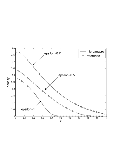
Figure 1: Left: numerical solutions in the kinetic and transition regimes, $\varepsilon=1,\,\varepsilon=0.5,\,\varepsilon=0.2$. The density for the micro/macro scheme coincides with the reference calculated with a highly resolved explicit scheme. Right: numerical solutions in the transition and diffusion regimes. The density for the micro/macro scheme coincides with the reference. For $\varepsilon=0.05$, the reference is calculated with the highly resolved explicit scheme. For $\varepsilon=0.0001$, the reference is calculated by the diffusion equation with the Chandrasekhar value at the boundary. Both figures are plotted at time $t=0.4$ and all micro/macro schemes are used with a uniform grid of $100$ points in $x$.

Acknowledgement.  The authors were supported by the french ANR project CBDif. M. Lemou acknowledges support from the project ’Défis émergents’ funded by the university of Rennes 1. F. Méhats acknowledges support from the french ANR project QUATRAIN and from the INRIA project IPSO.

References

- [1] M. Bennoune, M. Lemou, L. Mieussens, Uniformly stable numerical schemes for the Boltzmann equation preserving compressible Navier-Stokes asymptotics, J. Comput. Phys. 227(8) 3781-3803 (2008)
- [2] B. Dubroca, A. Klar, Prise en compte d’un fort déséquilibre cinétique par un modèle aux demi-moments [Half-moment model taking into account strong kinetic non-equilibrium]. C. R. Math. Acad. Sci. Paris 335 (2002), no. 8, 699–704.
- [3] S. Jin, L. Pareschi, G. Toscani, Uniformly accurate diffusive relaxation schemes for multiscale transport equations. SIAM J. Num. Anal., 38 (2000), pp. 913-936.
- [4] A. Klar, An asymptotic-induced scheme for nonstationary transport equations in the diffusion limit. SIAM J. Num. Anal., 35 (1998), pp. 1073-1094.
- [5] A. Klar, An asymptotic preserving numerical scheme for kinetic equations in the low Mach number limit. SIAM J. Num. Anal., 36 (1999), pp. 1507-1527.
- [6] M. Lemou, L. Mieussens, A new asymptotic preserving scheme based on micro-macro formulation for linear kinetic equations in the diffusion limit, SIAM J. Sci. Comp. 31(1) 334-368 (2008)
- [7] M. Lemou, Relaxed micro/macro schemes for kinetic equations. Comptes Rendus Mathematique, Volume 348, Issues 7-8, April 2010, Pages 455-460.
- [8] M. Lemou, F. Méhats, Asymptotic Preserving schemes for kinetic equations including boundary layers, in preparation.