Multiscale Simulation of History Dependent Flow in Polymer Melt

Abstract

We have developed a new multiscale simulation technique to investigate history-dependent flow behavior of entangled polymer melt, using a smoothed particle hydrodynamics simulation with microscopic simulators that account for the dynamics of entangled polymers acting on each fluid element. The multiscale simulation technique is applied to entangled polymer melt flow around a circular obstacle in a two-dimensional periodic system. It is found that the strain-rate history-dependent stress of the entangled polymer melt affects its flow behavior, and the memory in the stress causes nonlinear behavior even in the regions where ${\rm Wi}\leq 1$. The spatial distribution of the entanglements $\langle Z\rangle$ is also investigated. The slightly low entanglement region is observed around the obstacle and is found to be broaden in the downstream region.

Industrial products using polymeric materials have become increasingly integral to our lives. One of the important characteristics of thermo-plastic polymeric material is that it can be easily molded and processed by controlling its state from a solid to a melt, which is beneficial in a variety of practical applications. The melt state of polymeric material can exhibit a lot of characteristic phenomena, e.g., die-swell and rod-climbingBoger_Walters , depending on the dynamic response of the polymer’s microscopic internal states under an imposed strain or strain-rate.

Predicting the flow of polymeric fluid is difficult because the macroscopic flow behavior depends heavily on the dynamic behavior of the microscopic internal states, and the states of polymers with very high molecular weight are complex at the microscopic level. When a polymer melt consists of polymers with a molecular weight $M$ higher than the entanglement molecular weight $M_{\rm e}$, the polymer molecules are entangled with each other, and the relaxation time of the polymer conformation is long compared to that of dilute polymer solutions because of the entanglement. Therefore, it is difficult to predict the rheological behavior, even for a homogeneous bulk entangled polymer melt, using molecular dynamics approaches without any coarse-graining procedures for the microscopic internal degrees of freedom. Reptation theoryEdwards1967 ; deGennes1971 ; DE1986 , in which a polymer chain is coarse-grained to a tube confined by the surrounding polymer chains, explains the complex behavior of entangled polymer melt composed of mono-disperse linear polymers. To apply the concept of a tube to a wider variety of polymers, the original reptation theory has been improved by introducing several important physical mechanismsMLD1998 ; IM2001 ; IM2002 ; Likhtman2003 . Extended reptation theory based on the Fokker-Planck equation for tube segments succeeds in explaining many experimental resultsMLD1998 ; IM2001 ; IM2002 ; Likhtman2003 . However, it is difficult to apply the theory to arbitrary polymer melts because it is too mathematically complex to incorporate the molecular pictures of polymers of arbitrary architectures into the Fokker-Planck equation. On the other hand, Langevin stochastic models based on reptation theory using the complex molecular configurations have been developed and can reproduce the rheological properties of various polymeric materials with branches and/or molecular weight distributionsMasubuchi2001 ; SLTM2001 ; DT2003 ; Likhtman2005 . These models use efficient numerical computation to predict the bulk rheology of polymer melts; however, they are not applicable to macroscopically inhomogeneous flows only by themselves. The macroscopic flow behavior of polymer melt is usually predicted using a fluid dynamics simulation with a constitutive equation that describes a nonlinear and history dependent relationship between the stress and strain-rate fields to represent complex fluids without microscopic details. However, no general constitutive equation that is applicable to entangled polymer melts with arbitrary polymer architecture exists because a general polymer melt, e.g., polymers with branches and/or molecular weight distributions, has extremely complex molecular states, which makes the stress response unpredictable even in simple flow patterns. As described above, each of the microscopic and macroscopic approaches has limited applications. Recently, a molecularly derived constitutive equation technique is developed for low-molecular polymer melts without entanglementsIlg2011 . If it is generalized to a variety of polymer architectures, the technique can be attractive and useful. However, it is in an early phase of development toward generalization.

As an alternative to using a constitutive equation, we propose a new simulation technique that incorporates Langevin course-grained simulatorsMasubuchi2001 ; SLTM2001 ; DT2003 ; Likhtman2005 into a fluid dynamics simulation. This approach is a type of micro-macro simulations that were mainly developed for dilute polymer solutions in which the stress tensor of each fluid element is obtained from a microscopic simulationCONNFFESSIT ; LPM ; BCF , and applied not to dilute polymer solutions but to well entangled polymer melts here. In contrast to the dilute polymer solutions, the polymer melts have entanglement interactions between neighboring polymers. In order to investigate the entangled polymer melts using the micro-macro simulation, we need to satisfy (i) a local stress tensor is represented by an ensemble of a sufficiently large number of entangled polymers and to consider (ii) strong correlation among the polymers in an ensemble because of the entanglements. The advection of the stress, $(\bm{\mathrm{v}}\cdot\bm{\mathrm{\nabla}})\bm{\mathrm{\sigma}}$, in the Eulerian description is well established in any fields. However, it only advects the macroscopic quantity of the stress (the statistical conformation tensor) without involving microscopic molecules themselves. Because the correlations among polymers, namely the entanglements, intrinsically affect their macroscopic properties in the entangled polymer melts, the advection of an ensemble of polymers correlating at the microscopic level should be consistently managed with the advection of the macroscopic variables. Therefore, we adopt a Lagrangian fluid particle methodEKH2002 ; EEF2003 ; MT2010 to ensure the advection of the ensemble of entangled polymers. Each ensemble of entangled polymers is assigned on each fluid element. The advection of microscopic details is essential to the description of the macroscopic flow behavior for entangled polymer melts because the conformations of entangled polymers are constrained by and correlated to the surrounding polymers. Note that the Eulerian techniques can still be useful even for entangled polymer melts when the system has a translational symmetryYY2009 ; YY2010 .

To maintain the information pertaining to entanglement and deformation in polymers, we perform a Lagrangian fluid particle simulation in which each fluid particle has a microscopic level simulator that accounts for the internal states of the fluid particleMT2010 . Assuming that the polymer melt is an isothermal and incompressible fluid, the governing equations for the $i$-th fluid particle that constitutes the polymer melt are given by the following equations;

$$\rho_{i}\frac{{\rm d}\bm{\mathrm{v}}_{i}}{{\rm d}t}=\bm{\mathrm{\nabla}}\cdot\bm{\mathrm{\sigma}}_{i}-\bm{\mathrm{\nabla}}p_{i}+\bm{\mathrm{F}}^{\rm b}, \quad\frac{{\rm d}\bm{\mathrm{r}}_{i}}{{\rm d}t}=\bm{\mathrm{v}}_{i},$$ (1)

$$\bm{\mathrm{\sigma}}_{i}\equiv\bm{\mathrm{\sigma}}_{i}(\mathcal{Q}_{i}),$$ (2)

where $\bm{\mathrm{F}}^{\rm b}$ is a body force and the pressure $p_{i}\equiv p_{i}(\{\rho_{i}\})$ is properly considered to guarantee the incompressibility. These equations are solved using macroscopic variables, except for Eq. (2). The local stress tensor $\bm{\mathrm{\sigma}}_{i}$ depends on a microscopic ensemble $\mathcal{Q}_{i}$ of entangled polymers, which represent entangled states of polymers under an instantaneous local strain-rate $\bm{\mathrm{\kappa}}_{i}\equiv(\bm{\mathrm{\nabla}}\bm{\mathrm{v}})^{\rm T}_{i}$.

The slip-link modelSLTM2001 ; DT2003 is a simulation model that can accurately describe the dynamics of entangled polymers. The model is composed of confining tubes with some entanglement points, called slip-links, which confine a pair of polymers and represent effective constraints in virtual space. The average number of slip-links or entanglements on a polymer at the equilibrium state is represented as $\langle Z\rangle_{\rm eq}\equiv M/M_{\rm e}$. In the simulation, we trace the configurations of confining tubes constrained by the slip-links. The slip-links are relatively convected each other and the confining tubes are deformed according to the macroscopically obtained local velocity gradient tensor $\bm{\mathrm{\kappa}}$. The reptations of polymers generate or eliminate slip-links. For given chain configurations, the stress tensor $\bm{\mathrm{\sigma}}^{\rm p}$ derived from deformations of entangled polymers is calculated from $\sigma_{\alpha\beta}^{\rm p}=\sigma_{\rm e}\sum_{j}\langle r_{j\alpha}^{\rm s}r_{j\beta}^{\rm s}/|\bm{\mathrm{r}}_{j}^{\rm s}|\rangle/a_{\rm s}$ where $a_{\rm s}$ is the unit length of the slip-link model and $r_{j\alpha}^{\rm s}$ is the $\alpha$-component of the $j$-th tube segment vector connecting adjacent slip-links along a polymer. The unit of stress $\sigma_{\rm e}$ in the slip-link model relates to the plateau modulus $G_{\rm N}$ as follows: $\sigma_{\rm e}=(15/4)G_{\rm N}$DT2003 . The slip-link model has two characteristic time-scales: the Rouse relaxation time $\tau_{\rm R}$ and the longest relaxation time $\tau_{\rm d}$. The Rouse relaxation time $\tau_{\rm R}$ and the longest relaxation time $\tau_{\rm d}$ relate to $\langle Z\rangle_{\rm eq}$ as follows: $\tau_{\rm R}=\langle Z\rangle_{\rm eq}^{2}t_{\rm e}$ and $\tau_{\rm d}\propto\langle Z\rangle_{\rm eq}^{3.4}t_{\rm e}$DT2003 ; DE1986 , where $t_{\rm e}$ is the time unit of the slip-link model. The contour length relaxation of a confining tube occurs on the time-scale of $\tau_{\rm R}$, while the orientational relaxation occurs on the time-scale of $\tau_{\rm d}$. These two characteristic times appear in the stress relaxation.

Each polymer simulator describing a fluid particle computes the polymer configurations at each time step, and the recorded configurations are used as the initial conditions of the next time step. Typically, the macroscopic time unit $t_{\rm macro}$ and microscopic time unit $t_{\rm micro}$ have a large time-scale gap, and therefore the macroscopic time unit $t_{\rm macro}$ must be divided into $Nt_{\rm micro}$. Because the slip-link model used here is sufficiently coarse-grained and the time unit $t_{\rm e}$ can be the same as the time-scale of the macroscopic fluid $t_{\rm macro}$, we employ $t_{\rm macro}=t_{\rm micro}\equiv t_{\rm e}$.

Note that we set the local stress of the macroscopic fluid to $\bm{\mathrm{\sigma}}=\bm{\mathrm{\sigma}}^{\rm p}+\bm{\mathrm{\sigma}}^{\rm d}$, where $\bm{\mathrm{\sigma}}^{\rm d}$ is an extra dissipative stress tensor. Because the slip-link model is a Langevin coarse-grained model based on reptation theory, microscopic dynamics smaller than a tube segment are treated as a random force exerted on a slip-link, and the contribution from the microscopic dynamics does not explicitly appear in the stress tensor of the slip-link model. We assume the dissipative stress $\bm{\mathrm{\sigma}}^{\rm d}$ to be the Newtonian viscosity $\eta_{\rm{}_{d}}\bm{\mathrm{D}}$, where $\bm{\mathrm{D}}\equiv\bm{\mathrm{\kappa}}+\bm{\mathrm{\kappa}}^{\rm T}$ is a strain-rate tensor.

The main procedures of our simulation are summarized as follows: (1) Update $\{\bm{\mathrm{v}}_{i}\}$, $\{\bm{\mathrm{r}}_{i}\}$ at the macroscopic level. (2) Calculate $\{\rho_{i}\},\{\bm{\mathrm{\kappa}}_{i}\}$ at the macroscopic level. (3) Obtain $\{p_{i}\}$ from the density distribution $\{\rho_{i}\}$ at the macroscopic level. (4) Update the local slip-links of the $i$-th fluid particle under the local strain-rate $\bm{\mathrm{\kappa}}_{i}$ and then obtain $\bm{\mathrm{\sigma}}_{i}$ from the resulting configuration of the slip-link model. This procedure is executed on each fluid particle in turn. (5) Calculate $\{\bm{\mathrm{\nabla}}\cdot\bm{\mathrm{\sigma}}_{i}\}$ and $\{\bm{\mathrm{\nabla}}p_{i}\}$ at the macroscopic level. (6) Return to (1).

We update $\{\bm{\mathrm{v}}_{i}\}$, $\{\bm{\mathrm{r}}_{i}\}$ by integrating Eq. (1). We calculate the density at the position of each particle in the new configuration using a method in the usual smoothed particle hydrodynamics techniqueSPH : $\rho_{i}=\sum_{j}m_{j}W(|\bm{\mathrm{r}}_{j}-\bm{\mathrm{r}}_{i}|,h)$, where $m_{i}$ is the mass of the $i$-th particle and $W(|\bm{\mathrm{r}}|,h)$ is a Gaussian-shaped function with cutoff length $2h$. The deviation of the local density from the initial constant density $\rho_{0}$ results in a local pressure force $-\bm{\mathrm{\nabla}}p$. To obtain the spatial derivative of the velocity field, stress field, and pressure field ($\bm{\mathrm{\nabla}}\bm{\mathrm{v}},\bm{\mathrm{\nabla}}\cdot\bm{\mathrm{\sigma}},\bm{\mathrm{\nabla}}p$), we use a technique that was developed for modified smoothed particle hydrodynamicsMSPH ; FPM .

To demonstrate the efficiency of the proposed multiscale simulation, we consider a system in which the flow history can affect the flow behavior. One such system is a polymer melt flow around an infinitely long cylinder oriented in the $z$-direction with a radius $r_{\rm c}$, which flows in the $x$-direction. Because of the symmetry of the system, we can treat the system as two-dimensional, and the flow can be described as two-dimensional flow in the $xy$-plane. We assume a non-slip boundary condition for the velocity on the surface of the cylinder and periodic boundary conditions at the boundaries of the system. The dimensionless parameters governing the problem are the Reynolds number ${\rm Re}=\rho|\bar{\bm{\mathrm{v}}}|r_{\rm c}/\eta^{0}$, the Weissenberg number ${\rm Wi}=\tau_{\rm d}D_{xy}$, and the viscosity ratio $\eta_{\rm d}/\eta^{0}$, where $\bar{\bm{\mathrm{v}}}$ is the average flow velocity. The zero shear viscosity $\eta^{0}$ of the polymer melt is given by $\eta_{\rm p}^{0}+\eta_{\rm d}$, where $\eta_{\rm p}^{0}$ is the zero shear viscosity of a polymer melt described only by the slip-link model. From the rheological data shown in Fig. 1 (a), which were derived from the slip-link simulation with $\langle Z\rangle_{\rm eq}=7$ in the bulk, we obtain the longest relaxation time $\tau_{\rm d}\simeq 200t_{\rm e}$ and the zero shear viscosity $\eta_{\rm p}^{0}\simeq 17.5\sigma_{\rm e}t_{\rm e}$. The cylinder radius $r_{\rm c}$ was set to $3a$, where $a$ is the unit length in the fluid particle simulation, and we assign the unit mass $m$ to all fluid particles. The wall of the cylinder consists of fixed fluid particles evenly spaced on the perimeter. Each fluid particle consists of 10000 polymers, enough to describe the bulk rheological properties of the polymer melt under an imposed shear and/or extensional deformationMT2010 . About 900 fluid particles with 10000 polymers each are evenly placed initially in the system and then move according to Eq. (1); therefore, we need to simultaneously solve the dynamics of 9000000 polymers. Because the diffusive motion of the center of mass of a single polymer is negligible compared to the translational motion of the center of mass of an ensemble of entangled polymers, we neglect any transportation of polymers between adjacent fluid particles. With this assumption, each slip-link simulation can be performed independently of the others, making parallel computing effective in this multiscale simulation.

Figure 1: (a) Rheological data and (b) relaxation modulus $G(t)$ obtained from the slip-link simulation with $\langle Z\rangle_{\rm eq}=7$ in the bulk. The storage modulus $G^{\prime}$ (dashed line), the loss modulus $G^{\prime\prime}$ (dotted line), and the complex viscosity $\eta^{*}$ (solid line) are plotted against the angular frequency $\omega$ in (a). The magnitude of the complex viscosity, $|\eta^{*}|=\sqrt{G^{\prime 2}+G^{\prime\prime 2}}/\omega$, is considered to be the shear viscosity $\eta$ of the low shear-rate region (Cox-Merz rule). The normalized relaxation modulus $G(t)/G(0)$ (solid line) and a single exponential curve with a relaxation time $\tau$ (dashed line) are plotted against the normalized time $t/\tau$ in (b).

Under the body force $\bm{\mathrm{F}}^{\rm b}/(\eta^{0}/at_{\rm e})=(5.0\times 10^{-4},0)$, the flow becomes steady-state in about $1000t_{\rm e}$. The average flow velocity $\bar{\bm{\mathrm{v}}}$ in steady-state in this system is nearly equal to $(0.04,0)a/t_{\rm e}$ for a fully Newtonian flow $\eta^{0}=\eta_{\rm d}$ ($\bm{\mathrm{\sigma}}^{\rm p}=0$), and $(0.055,0)a/t_{\rm e}$ for a polymer melt flow with $\langle Z\rangle_{\rm eq}=7$ and $\eta_{\rm d}/\eta^{0}=0.1$. In both cases, ${\rm Re}$ is less than 0.2, and the flow is laminar. In the polymer melt case, the average flow velocity is higher than that of Newtonian flow, i.e., the flow exhibits shear thinning behavior because of ${\rm Wi}>1$ in the vicinity of the cylinder.

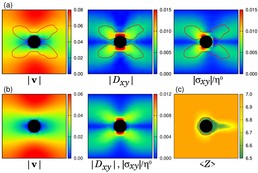
Figure 2: Color contour maps of time-averaged magnitudes of the velocity field $|\bm{\mathrm{v}}|[a/t_{\rm e}]$, strain-rate $|D_{xy}|[1/t_{\rm e}]$, and shear stress over the zero shear viscosity $|\sigma_{xy}|/\eta^{0}[1/t_{\rm e}]$ for (a) the polymer melt with $\langle Z\rangle_{\rm eq}=7$ and $\eta_{\rm d}/\eta^{0}=0.1$ and (b) the Newtonian fluid with $\eta^{0}=\eta_{\rm d}$ in steady-state. Figure (c) shows $\langle Z\rangle$ in the polymer melt. The regions inside the red lines in (a) correspond to ${\rm Wi}\geq 1$ and those in (c) to $\tau_{\rm R}\dot{\gamma}\geq 1$ where $\dot{\gamma}\equiv\sqrt{{\rm Tr}(\bm{\mathrm{\kappa}}^{\rm T}\bm{\mathrm{\kappa}})}$.

To investigate the velocity field $\bm{\mathrm{v}}$, strain-rate $D_{xy}$, and shear stress $\sigma_{xy}$ in steady-state, we employ a linear interpolation to transform the data at the particle positions into the values at regular lattice points and then time-average the data evaluated at the lattice points. To eliminate the noise of the data, the time-averaging was carried out from 1000$t_{\rm e}$ to 2000$t_{\rm e}$. Figure 2 shows the spatial distributions of $|\bm{\mathrm{v}}|$, $|D_{xy}|$ and $|\sigma_{xy}|/\eta^{0}$ in steady-state for (a) the polymer melt with $\langle Z\rangle_{\rm eq}=7$ and $\eta_{\rm d}/\eta^{0}=0.1$ and (b) the Newtonian fluid with $\eta^{0}=\eta_{\rm d}$.

Reflecting laminar behavior, the magnitudes of $\bm{\mathrm{v}}$ and $D_{xy}$ in Fig. 2 appear to be nearly symmetric between the upstream and downstream regions unlike $\sigma_{xy}$. In Fig. 2 (a), the nonlinear relationship between $\sigma_{xy}$ and $D_{xy}$ is observed near the cylinder where ${\rm Wi}>1$ because of shear thinning. Moreover, the shear stress $\sigma_{xy}$ of the polymer melt exhibits an apparent asymmetry between the upstream and downstream regions. In general, the viscoelastic stress relates to the shear-rate through the relaxation modulus according to the following equation: $\sigma(t)=\int_{-\infty}^{t}dt^{\prime}G(t-t^{\prime})\dot{\gamma}(t^{\prime})$; the stress depends on the flow history.

Figure 3: Stream lines (solid line(A) and dashed line(B)) obtained from the time-averaged velocity field with particle tracking are plotted against position in (a). These stream lines are in the region where ${\rm Wi}\leq 1$. The strain-rate $D_{xy}$ and the shear stress $\sigma_{xy}$ along the stream lines are plotted against the elapsed particle tracking time in (b). Each line type corresponds to each stream line.

We investigate the behavior of $\sigma_{xy}$ and $D_{xy}$ on two typical stream lines (A: solid line and B: broken line shown in Fig. 3 (a)) in the region where ${\rm Wi}\leq 1$. Figure  3 (b) shows $\sigma_{xy}$ and $D_{xy}$ along these stream lines and plots them against the elapsed particle tracking time. The time origin $t=0$ is set to $t_{\rm min}$, when the strain-rate $D_{xy}$ is at a minimum in each stream line. A nonlinear relationship between $\sigma_{xy}$ and $D_{xy}$ is not evident in either stream line because ${\rm Wi}\leq 1$; however, the minimum of $\sigma_{xy}$ appears to be shifted from that of $D_{xy}$ by a time difference $t_{\Delta}$. Applying a step shear strain $\gamma=0.5$ to the slip-link model with $\langle Z\rangle_{\rm eq}=7$ in the bulk, we obtain the relaxation modulus $G(t)\equiv\sigma(t)/\gamma$ shown in Fig. 1 (b). The stress relaxation time $\tau$ is estimated to be $\tau\simeq 50t_{\rm e}(\simeq\tau_{\rm R})$ when $G(t=\tau)/G(0)=1/e$. The time difference $t_{\Delta}$ is found to be nearly equal to $\tau$.

Finally, we investigate the spatial distribution of entanglements $\langle Z\rangle$ shown in Fig. 2 (c). In the vicinity of the cylinder, the entanglements slightly decrease. When $\tau_{\rm R}\dot{\gamma}\geq 1$, polymer’s contour length is highly extended. The extended polymer longer than $\langle Z\rangle_{\rm eq}a$ is easy to shrink, which causes disentanglement. In the upstream and downstream regions around the cylinder, the reduction of $\langle Z\rangle$ is also observed because of nonzero $|D_{yy}|$. The flow advection broadens the region where $\langle Z\rangle<\langle Z\rangle_{\rm eq}$ in the downstream region. The tail length in the downstream region is roughly estimated to be $\tau_{\rm R}|\bar{\bm{\mathrm{v}}}|\sim r_{\rm c}$.

Using the Lagrangian particle method to trace and maintain the entire configurations of polymers, we have been able to describe the memory effect in the polymer melt flow. The presented multiscale simulation is applicable to various polymer melts, because the slip-link model or the alternative course-grained modelsMasubuchi2001 ; Likhtman2005 can address a variety of polymer architectures, e.g., linear and/or branched polymers, polymer blends, and polydispersed polymers. The multiscale simulation is advantageous because it employs a fully Lagrangian method at the macroscopic level, while conventional micro-macro techniques which have difficulties accounting for the macroscopic advection of microscopic internal states.

- (1) D. V. Boger and K. Walters, Rheological Phenomena in Focus, Elsevier, (1993).
- (2) S. F. Edwards, Proc. Phys. Soc., 92, 9, (1967).
- (3) P.-G. de Gennes, J. Chem. Phys., 55, 572, (1971).
- (4) M. Doi and S. F. Edwards, The theory of polymer dynamics., Oxford University Press, (1986).
- (5) D. W. Mead et al., Macromol., 31, 7895, (1998).
- (6) G. Ianniruberto and G. Marrucci, J. Rheol., 45, 1305, (2001).
- (7) G. Ianniruberto and G. Marrucci, J. Non-Newton. Fluid. Mech., 102, 383, (2002).
- (8) A. E. Likhtman and R. S. Graham, J. Non-Newton. Fluid. Mech., 114, 1, (2003).
- (9) Y. Masubuchi et al., J. Chem. Phys., 115, 4387, (2001).
- (10) S. Shanbhag et al., Phys. Rev. Lett., 87, 195502, (2001).
- (11) M. Doi and J. Takimoto, Phil. Trans. R. Soc. Lond. A, 361, 641, (2003).
- (12) A. E. Likhtman, Macromol., 38, 6128, (2005).
- (13) P. Ilg and M. Kröger, J. Rheol., 55, 69, (2011).
- (14) M. Laso and H. Öttinger, J. Non-Newton. Fluid. Mech., 47, 1, (1993).
- (15) P. Halin et al., J. Non-Newton. Fluid. Mech., 79, 387, (1998).
- (16) M. A. Hulsen et al., J. Non-Newton. Fluid. Mech., 70, 79, (1997).
- (17) M. Ellero et al., J. Non-Newton. Fluid. Mech., 105, 35, (2002).
- (18) M. Ellero et al., Phys. Rev. E, 68, 041504, (2003).
- (19) T. Murashima and T. Taniguchi, J. Polym. Sci. B, 48, 886, (2010).
- (20) S. Yasuda and R. Yamamoto, Euro. Phys. Lett., 86, 18002, (2009).
- (21) S. Yasuda and R. Yamamoto, Phys. Rev. E, 81, 036308, (2010).
- (22) J. Monaghan, Rep. Prog. Phys., 68, 1703, (2005).
- (23) G. Zhang and R. Batra, Comput. Mech., 34, 137, (2004).
- (24) M.B. Liu et al., Appl. Math. Model, 29, 1252, (2005).