Digital watermarking : An approach based on Hilbert transform

Abstract

ABSTRACT

Most of the well known algorithms for watermarking of digital images involve transformation of the image data to Fourier or singular vector space. In this paper, we introduce watermarking in Hilbert transform domain for digital media. Generally, if the image is a matrix of order $m$ by $n$, then the transformed space is also an image of the same order. However, with Hilbert transforms, the transformed space is of order $2m$ by $2n$. This allows for more latitude in storing the watermark in the host image. Based on this idea, we propose an algorithm for embedding and extracting watermark in a host image and analytically obtain a parameter related to this procedure. Using extensive simulations, we show that the algorithm performs well even if the host image is corrupted by various attacks.

I Introduction

A large amount of accessible information today is available in one or the other multimedia formats. While this serves the purpose of easier dissemination of data, this also makes it vulnerable for misappropriation and misuse. Hence, it is all the more important to protect intellectual property rights of the content available in various digital formats. Digital watermarking Langelaar ; Cox-1 is a popular method by which the owners of the data, in any multimedia format, can embed their logo, trademark or some proprietary information Zeng-2 ; Petitcolas in a way that can either be visible or invisible to a general user. This information can be later retrieved for verification purposes or in case of conflicting claims on the ownership of data Craver ; Piva-2 ; Zeng-1 .

Thus, when applied to the case of digital images, digital watermarking technique consists of (i) an algorithm to embed a watermark image on a host image and (ii) an algorithm to retrieve the embedded watermark with least distortion. Ideally, we would expect that the algorithms be robust against any manipulation of the original data and it should also be designed to render any illegal retrieval of watermark a futile exercise. The field of digital watermarking has been the focus of research attention for more than a decade now. This is partly due to the proliferation of multimedia formats as well as new tools, both commercial and open source, to manipulate them. In this paper, we focus on the invisible watermarking of digital images using the Hilbert transform technique.

Watermarking techniques for digital images can be broadly classified into two categories, namely, the spatial domain techniques and transform domain techniques depending on which domain the watermark is embedded. Typically, in spatial domain techniques the watermark is embedded in those part of the data that do not distort the host image in any significant way. For instance, some of the well-known spatial domain techniques are least significant substitution Cox-2 ; Podilchuk and the correlation based approach Kallel-2 ; Raval . In least significant substitution technique, the watermark is embedded by replacing the least significant bits of the image data with the bits of the watermark data. There are many variants of this technique. In correlation based approach the watermark is converted to a pseudo-random noise (PN) sequence which is then weighted and added to the host image with a gain factor. For detection, the watermarked image is correlated with the watermark image. In the transform domain techniques, the watermark is embedded in those parts of the transformed host image which do not distort the image significantly.

One of the earliest transform domain techniques is the one based on discrete cosine transform (DCT) Barni-1 ; Chu ; Hernandez ; Dickinson ; Piva-1 . In DCT, the image is decomposed in terms of various frequency bands and watermarks are embedded in the middle frequency bands which are not significant for the host image. Further, image transformations do not affect the watermark placed in those bands. DCT based methods are generally robust, particularly against JPEG and MPEG compression. The techniques based on wavelet decomposition are similar in spirit to DCT with the additional feature that the multi-resolution character of the wavelets allows graded information to be stored at various resolutions. For instance, in Kundur wavelet coefficients of the image and the watermark at different levels of resolution are added together within the constraint of the so-called human-visual model. A review of wavelets based techniques is available in Barni-2 ; Wang ; Karras ; Taweel ; Kundur-2 . There is yet another method of digital watermarking based on singular value decomposition (SVD) techniques Chang-1 ; Chang-2 ; Liu ; Gorodetski ; Chandra ; Sun ; Yongdong ; Agarwal ; Shieh ; Andrews . In contrast to DCT and wavelets based techniques, the advantage of singular value decomposition based methods is that they provide a transform space that is tailor made for the given image data matrix. Both in the DCT and wavelets, the basis for the transform space is a fixed set of functions. In the SVD, it must be calculated from the given data and the singular vectors so calculated form an optimal basis for the image matrix in the least square sense. It is worth mentioning that some authors have resorted to hybrid techniques i.e., algorithms based simultaneously on different domains to improve the watermarking results Po ; Ganic-1 ; Ganic-2 ; Gaurav .

In this present work, we propose a new scheme for watermarking digital images using the Hilbert transform. The analytic signal $\hat{s}(t)$ associated to a signal $s(t)$ is,

$$\hat{s}(t)=s(t)+is_{H}(t)$$ (1)

where $s_{H}(t)$ is the Hilbert transform of $s(t)$. Clearly, $\hat{s}(t)$ can be written in phase-amplitude form as $A(t)e^{i\theta(t)}$. If the signal changes sufficiently slowly, then the phase of the analytic signal is negligible. Typically, most images have slowly varying pixel values except at the edges. In such a scenario, we can expect the phase to be negligible most of the time and the matrix of phase values will be sparse. Hence a good amount of information can be embedded in the phase of the analytic signal associated to the image. Since only the phase of the analytic signal is proposed to be used for embedding the watermark, it is likely to be highly imperceptible for visual perception. This is one of the key requirements of ideal watermarking algorithms. In addition, this also provides a large space for embedding the watermark which is useful for creating redundant watermark distributed throughout the Hilbert transformed space. This makes the algorithm more robust against attacks. This is the main idea underlying the present scheme and to the best of our knowledge the Hilbert transform has not been used for watermarking purposes before.

Further, our proposal is a non-blind scheme, which implies that to recover the watermark from the watermarked image, we require both the original as well as the watermark image. This is not necessarily a restrictive requirement as there are many situations in which this scenario is valid, such as in ownership litigations. In many such cases, the owner keeps a copy of both the original host image and the watermark. In addition, non-blind scheme also makes detection of watermark in an arbitrary image difficult if the watermark image is not available.

The rest of the paper is organized as follows. In the next section, we introduce the proposed method of digital watermarking. In Sec.III, we provide the formula to optimize the scaling factor. Section IV describes the results of numerical simulation, while Sec. V describes robustness of the algorithm. Section VI gives a summary and concluding remarks.

II Watermarking using the Hilbert transform

Given any arbitrary signal $s(t)$, as a function of time $t$, we can construct an analytic signal of the form

$$\hat{s}(t)=s(t)+is_{H}(t)=A(t)e^{i\theta(t)}$$ (2)

where $s_{H}(t)$ is the Hilbert transform of $s(t)$. It is defined in terms of the Cauchy principal value (P.V) of the integral

$$s_{H}(t)=\frac{1}{\pi}\mbox{P.V}\int_{-\infty}^{\infty}\frac{s(\tau)}{t-\tau}~{}d\tau$$ (3)

provided this integral exists. In general, Hilbert transform has a wide range of applications, in particular, in the area of signal processing Stefan . In signal processing, the Hilbert transform $\bf{z_{H}}$ of a discrete signal $\bf{z}$ is defined as the output of a linear filter with the frequency response $H(\omega)$ given by

$$H(\omega)=\left\{\begin{array}[]{l l}i,&\quad-\pi<\omega<0\\ -i,&\quad 0<\omega<\pi\\ 0,&\quad\omega=-\pi,0,\pi\\ \end{array}\right.$$ (4)

In the context of this work, let $\mathbf{z}$ denote a signal vector of size $n\times 1$ as a function of position (in arbitrary units). For instance, $\mathbf{z}$ would represent one column of pixel values of an image matrix $\mathbf{Z}$ of order $n\times m$. Then, the analytic signal $\hat{z}$ associated with $\mathbf{z}$ is $\bf{z+iz_{H}}$, a complex valued signal with phase and amplitude. We intend to embed the watermark image in the phase component. We denote the amplitude and phase of this analytic signal by $n\times 1$ vectors $\mathbf{r_{z}}$ and $\mathbf{\theta_{z}}$ respectively. The inverse Hilbert transform consists of taking the real part $\mathbf{r_{z}}$ of this analytic signal. Hence we have,

$$\mathbf{z=r_{z}*\cos\theta_{z}},$$ (5)

where the $\mathbf{*}$ stands for element-wise multiplication and is not to be confused with usual matrix multiplication. Further, for any vector $\mathbf{\theta_{z}}$, the operation $\cos\mathbf{\theta_{z}}$ represents the cosine of every element of the vector.

Notice that the Hilbert transforms in two dimensions is not uniquely defined. Hence, in the watermarking algorithm presented below, we will treat the image matrix $\mathbf{Z}$ of size $n\times m$ as $n$ vectors and apply Hilbert transforms to each of the $n$ vectors. From a computational point of view, for the Hilbert transform of any image $\mathbf{Z}$, we are required to compute $n$ independent Hilbert transforms each with $m$ elements. However, for ease of notation, we present the algorithm using scalar elements instead of in vector notation. Now we will apply this to define Hilbert transform of an image matrix $\mathbf{Z}$ of size $n\times m$ with elements $Z_{ij},i=1,2,3,\ldots n,j=1,2,3,\ldots m$. Hence Eq.(5) will still continue to hold in the form

$$Z_{ij}=a_{ij}\cos\Theta_{ij},\quad i=1,2,3,\ldots n,\quad j=1,2,3,\ldots m.$$ (6)

In this, $a_{ij}$ are the amplitudes and $\Theta_{ij}$ are the phases obtained from vector-wise Hilbert transform applied on $\mathbf{Z}$.

II.1 Algorithm for embedding the watermark

In this section we describe the algorithm to embed a watermark image into another gray scale image of the same size using the Hilbert transform. Let the host image be represented by $\mathbf{Z}$ with elements $Z_{ij}$ and $\mathbf{W}$ denote the matrix of the watermark image with elements $W_{ij}$.

First, we perform the Hilbert transform of the original image $\mathbf{Z}$ and obtain the relation

$$Z_{ij}=a_{ij}\cos\Theta_{ij}.\;\;\;\;\;$$ (7)

Next, we do the same for the watermark image $\mathbf{W}$ to get

$$W_{ij}=b_{ij}\cos\Phi_{ij},$$ (8)

where $b_{ij}$ and $\Phi_{ij}$ are the phase and amplitude.

Now, we add the scaled amplitude $b_{ij}$ of the watermark to the phase $\Theta_{ij}$ of the original image to get

$$\theta_{ij}=\Theta_{ij}+\lambda b_{ij},$$ (9)

where $\lambda$ is the scaling factor. For typical images, the order of magnitude of $b_{ij}$’s is much larger than $\Theta{ij}$’s for all $i,j$ and hence $\lambda$ will have to be much smaller than unity in order to compensate for this difference in order of magnitudes.

Finally, we get the watermarked image $\mathbf{Z^{w}}$ as

$$Z^{w}_{ij}=a_{ij}\cos\theta_{ij}.$$ (10)

Thus equations (7)-(10) constitute the algorithm for watermarking using the Hilbert transform applied column-wise to an image matrix. We remark that this algorithm is motivated by the fact that most of the information about the image is encapsulated within the amplitude. The phases $\Theta_{ij}$, for all $i$ and $j$, contain very little information and can be thought of as a sparse matrix. Hence, we can store most of the information about the watermark without causing too much distortion in the original image by following the above strategy.

II.2 Algorithm for extracting the watermark

Given the watermarked image $\mathbf{Z^{w}}$, we can extract a (possibly corrupted) watermark if we have access to $\Theta_{ij},\Phi_{ij},a_{ij}$, for all $i$ and $j$, and the value of $\lambda$. This information is most easily available if one has access to the original image as well as the watermark image. As pointed out in a previous work of the first and the third author Agarwal , this is not a particularly restrictive assumption.

The extraction algorithm is just the reversal of the embedding algorithm given in the previous subsection. Starting from Eq. (10) we divide both sides by $a_{ij}$ and use the inverse cosine function to recover $\theta_{ij}$. By substituting for $\theta_{ij}$ using Eq. (9) we get for the amplitude of the watermarked image

$${\widetilde{b}}_{ij}=\frac{\cos^{-1}\left(Z^{w}_{ij}/a_{ij}\right)-\Theta_{ij}}{\lambda}.$$ (11)

Finally using Eq. (8), the extracted watermark image can be constructed as follows,

$$\widetilde{W}_{ij}=\widetilde{b}_{ij}\cos(\Phi_{ij}).$$ (12)

Thus, Eq. (12), along with Eq. (11) constitute the watermark extraction algorithm.

III Optimization of the scaling factor

The choice of the value of the scaling factor $\lambda$ plays an important role in our watermarking algorithm. If $\lambda$ is chosen too small, then the quality of embedding is good but that of the extracted watermark is poor. On the other hand, if $\lambda$ is too large, then extraction works well but embedding suffers. Hence, $\lambda$ needs to be chosen optimally to achieve a balance between these extremes. In general, this problem is a non-linear optimization problem and we shall describe an iterative method to produce a solution to it.

We shall use the mean square error (MSE) as a measure of the quality of embedding or extraction, and attempt to minimize the sum of the MSE from the embedding and extraction steps. First define the function $f(\lambda)$ as

$$f(\lambda)=\sum_{j=1}^{m}\sum_{i=1}^{n}\Big{[}(Z^{w}_{ij}-Z_{ij})^{2}+(\widetilde{W}_{ij}-W_{ij})^{2}\Big{]}.$$ (13)

With this notation, we need to find the value of $\lambda$ that minimizes $f(\lambda)$. Note that both $\mathbf{Z^{w}}$ and $\mathbf{\widetilde{W}}$ depend on $\lambda$. We also note that, in practice, converting $\mathbf{Z^{w}}$ to an image introduces a truncation error $\epsilon$, which, though negligible in the embedding step, affects the extraction step significantly.

Now, we use Eqs. (9) and (10) adjusted for the truncation error $\epsilon$ to get the following

$$\sum_{j=1}^{m}\sum_{i=1}^{n}(Z^{w}_{ij}-Z_{ij})^{2} =\sum_{j=1}^{m}\sum_{i=1}^{n}\big{[}a_{ij}\cos(\Theta_{ij}+\lambda b_{ij})$$

$$+\epsilon-a_{ij}\cos\Theta_{ij}\big{]}^{2}$$ (14)

$$\approx\sum_{j=1}^{m}\sum_{i=1}^{n}(-\lambda a_{ij}b_{ij}\sin\Theta_{ij}+\ldots)^{2},$$

where the terms involving $\epsilon$ and higher powers of $\lambda$ are ignored.

Similarly we use Eqs. (11) and (12) adjusted for $\epsilon$ to get

$$\sum_{j=1}^{m}\sum_{i=1}^{n}(\widetilde{W}_{ij}-W_{ij})^{2}$$

$$=\sum_{j=1}^{m}\sum_{i=1}^{n}\bigg{[}\frac{\cos^{-1}\big{[}\cos(\Theta_{ij}+\lambda b_{ij})+\epsilon/a_{ij}\big{]}-\Theta_{ij}}{\lambda}$$

$$\times\cos\Phi_{ij}-b_{ij}\cos\Phi_{ij}\Big{]}^{2}$$

$$=\sum_{j=1}^{m}\sum_{i=1}^{n}\left(\frac{\alpha(\lambda)\cos\Phi_{ij}}{\lambda}\right)^{2},$$ (15)

where $\alpha(\lambda)$ is given by

$$\alpha(\lambda)=\cos^{-1}(\cos(\Theta_{ij}+\lambda b_{ij})+\epsilon/a_{ij})-(\Theta_{ij}+\lambda b_{ij}).$$ (16)

With this preparation we return to the minimization of $f(\lambda)$. Our approach is to start with any initial value $\lambda=\lambda_{0}$ and produce successive values $\lambda_{1},\lambda_{2},\ldots$, each depending on the previous value, which converge to the desired minimum of $f(\lambda)$.

The method to produce $\lambda_{\ell+1}$ from $\lambda_{\ell}$ at the $\ell$-th step is as follows. First we use Eqs. (14) - (16) to approximate $f(\lambda)$ by $f_{\ell}(\lambda)$ as,

$$f_{\ell}(\lambda)=\sum_{j=1}^{m}\sum_{i=1}^{n}\Big{[}(a_{ij}b_{ij}\sin\Theta_{ij})^{2}\lambda^{2}+(\alpha(\lambda_{\ell})\cos\Phi_{ij})^{2}\lambda^{-2}\Big{]}.$$ (17)

Note that $f_{\ell}(\lambda)$ depend on $\lambda_{\ell}$. Next, we choose $\lambda_{\ell+1}$ to be the value at which $f_{\ell}(\lambda)$ attains its minimum. After a straightforward computation, we have the following,

$$\lambda_{\ell+1}=\left(\frac{\sum(\alpha(\lambda_{\ell})\cos\Phi_{ij})^{2}}{\sum(a_{ij}b_{ij}\sin\Theta_{ij})^{2}}\right)^{1/4}.$$ (18)

Thus Eq. (18) can be iterated for $\ell=0,1,\ldots$ starting from any initial value $\lambda_{0}$ till the desired level of convergence is achieved. In practice, this algorithm seems to have fast convergence. For example, for our test images it converges within $\ell=2$ steps to $\lambda=0.0018$ (upto 4 decimal places) for a wide range of initial values.

IV Numerical simulation

In this section we will apply our embedding and extraction algorithm to the host image shown in Fig. 1 and the watermark image in Fig. 1. Both these images have dimensions $512\times 512$. As pointed out earlier, the quality of the watermarked image improves and that of the extracted image deteriorates as the scaling parameter $\lambda\to 0$. This is borne out by the simulation results and can be clearly seen from the watermarked images shown in Figs. 2, 2, 2, 2, and 2 for $\lambda=0.1,0.01,0.0018,0.001,0.0001$ respectively. The corresponding extracted watermark images are shown in Figs. 2, 2, 2, 2, and 2. The simulations clearly demonstrate that the Hilbert transform based algorithm proposed in Eq. (7)-(10) and Eq. (11),(12) produces results whose visual quality is good and acceptable as a practical tool for watermarking digital images.

These results are quantified by means of peak signal to noise ratio (PSNR) and the root-mean-square error (RMSE) of the corresponding images. PSNR is used to evaluate the perceptual distortion of the proposed scheme. PSNR and RMSE is computed for the image difference matrix $\Delta_{ij}=I_{ij}-\widetilde{I}_{ij}$ for several values of $\lambda$. In our context, there are two possibilities, (a) $I_{ij}$ are the elements of host image and $\widetilde{I}_{ij}$ are the elements of watermarked image, and (b) $I_{ij}$ are the elements of watermark image and $\widetilde{I}_{ij}$ are the elements of extracted watermark. Then RMSE is defined as

$$\varepsilon=\sqrt{\frac{1}{mn}\sum_{i=1}^{m}\sum_{j=1}^{n}\Delta_{i,j}^{2}}\,.$$ (19)

We also define the PSNR, measured in decibels, as

$$p=10\log_{10}(\mbox{max}~{}z_{i,j}^{2}/\varepsilon^{2}),$$ (20)

where $\mbox{max}~{}z_{i,j}$ represents the maximum value of a matrix whose elements are $z_{i,j}$. Figure 3 depicts the combined RMSE versus lambda graph of the extracted and watermarked images. Notice that $\lambda=0.0018$ corresponds to a minima as predicted by the analysis in the previous section.

Figure 1: 1 Host image and 1 watermark image of size 512 $\times$ 512.

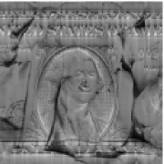
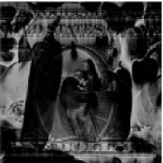
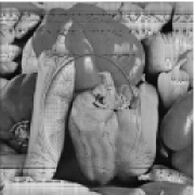
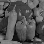
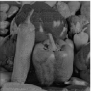
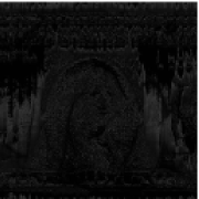
Figure 2: This panel shows the watermarked image on the left panel and the extracted watermark on the right panel for 2, 2 $\lambda=0.1$, 2, 2 $\lambda=0.01$, 2, 2 $\lambda=0.0018$, 2, 2 $\lambda=0.001$ and 2, 2 $\lambda=0.0001$.

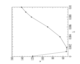
Figure 3: Mean square error versus $\lambda$ plot.

V Robustness of the algorithm

An important property of the watermarking algorithms is that they should be robust against various possible attacks. In this section, we will first embed the watermark in the host. The watermarked image will then be subjected to some attacks. After the attack has been carried out, the extraction algorithm is applied. We will subject our algorithm to the following major attacks (i) robustness against Additive Noise (ii) Cropping (iii) Gaussian Noise (iv) JPEG and JPEG 2000 compression (v) Median Filter (vi) Rotation (vii) Gamma Correction (viii) Intensity Adjustment (ix) Gaussian Blur (x) Contrast Enhancement (xii) Dilation (xiii) Scaling. The full list of attacks and their result is given in Table. (1). Before we proceed, at the very outset let us mention that all the images are taken to be of $512\times 512$ and the scaling factor is chosen to be $0.0018$ (optimal value). In particular, all the attacks are done on Fig. 2.

V.1 Additive Noise

Our first attack will be the addition of uniformly distributed noise to Fig. 2 resulting in the corrupted image shown in Fig. 4. Figure 4 shows the result of extracting the watermark. As can be noticed visually and also from the $p$ and $\epsilon$ values, the quality of the extracted watermark is quite good.

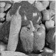
Figure 4: 4 Noise added watermarked image and 4 Extracted watermark.

V.2 Cropping

Cropping is the process of removing a portion of the image. In the present case we will remove a portion of the watermarked image and check if our extraction algorithm is able to extract the watermark. Figures 5 and 5 show the cropped watermarked images and the extracted watermark respectively. Though there is some residual effect of the host in the extracted image, it is worth noting that it appears only in the cropped portion of the image. The extracted image is unaffected by this residual effect of the host. We would also like to mention that we have carried out cropping for various percentages ($10\%$, $20\%$, $30\%$, $40\%$, $50\%$) of Fig. 2 and the extracted image is good.

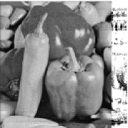
Figure 5: 5 Cropped watermarked image and 5 Extracted watermark.

V.3 Gaussian Noise

When Gaussian distributed noise is added to the watermarked image we obtain Fig. 6. The extracted image from this is shown in Fig. 6. Once again our extraction algorithm performs well and yields the watermark.

Figure 6: 6 Gaussian noise watermarked image and 6 Extracted watermark.

V.4 JPEG and JPEG 2000 Compression

JPEG compression jpegbook is one of the popular standards for encoding of digital images. This is also an important test that any watermarking algorithm has to defend itself against. We subject Fig. 2 to various percentages of JPEG compression and consequently extract the watermark from it. Figures 7, 7, 7, and 7 are JPEG compressed at $20\%$, $40\%$, $60\%$, and $80\%$ respectively. The extracted watermarks from the aforementioned compressed images are shown in Figs. 7, 7, 7, and 7 respectively. From the PSNR values indicated in the table, it is clear that the quality of the images extracted as well as the embedded is better when the compression is less. This seems normal since JPEG is a lossy compression method, the higher the compression, the more is the loss in information of the image and vice versa.

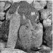
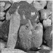
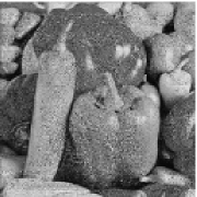
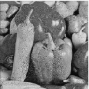
Figure 7: This panel shows the watermarked image on the left panel and the extracted watermark on the right panel for 7, 7 JPEG compressed $20\%$ watermarked image and Extracted watermark 7, 7 JPEG compressed $40\%$ watermarked image and Extracted watermark 7, 7 JPEG compressed $60\%$ watermarked image and Extracted watermark 7, 7 JPEG compressed $80\%$ watermarked image and Extracted watermark.

Now we focus on JPEG 2000 standard jp2book and show the results of attacks using JPEG 2000. This is a more recent standard for image compression and is based on wavelets and is much more efficient in reducing the size of images. Figures 8 and 8 show, the compressed watermarked image and the result of the extraction from it respectively at a JPEG 2000 ratio valued at two. The PSNR and RMSE plot for the watermarked image for various JPEG 2000 compression ratios is given in Fig. 9. Similarly the plot for the extracted watermark is given in Fig. 9. Just like the JPEG case, the results show a deterioration in the quality of the watermarked as well as of the extracted watermark images as the compression ratio is increased. However, the watermark can still be obtained even for very high compression ratios which could be attributed to the robustness of the algorithm.

Figure 8: 8 Watermarked image after JPEG 2000 compression (Compression Ratio 2) and 8 Extracted watermark.

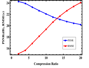
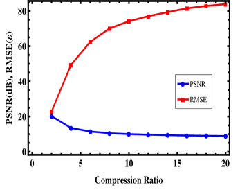
Figure 9: Graph depicting the variation of $p$ and $\epsilon$, for various compression ratios taken in the $x$ axis, 9 Between the original and the watermarked images and 9 Between the watermark and the extracted images.

V.5 Median Filter

Median filtering is used to remove outliers without reducing the sharpness of the image. It is similar to an averaging filter in which the value of the output pixel is the mean of the pixel values in the neighborhood of the corresponding input pixel. However, in the present method of median filtering, as one might have guessed, the value of an output pixel is determined by the median of the neighborhood pixels. The extracted watermark, Fig. 10, from the median filtered Fig. 10 shows that the proposed scheme is robust to such an attack.

Figure 10: 10 Median filtered watermarked image and 10 Extracted watermark.

V.6 Rotation

Figure 11 shows the result of rotating the watermarked image, Fig. 2, through one degree in the anti-clockwise direction. After this has been done we crop the four corners of the rotated image in order to keep the same size as the original image. Now when the extraction algorithm is applied, the resulting extracted watermark is shown in Fig. 11. Tests have been done for rotations by $2$ and $3$ degrees too. In these cases we are able to retrieve more than $50\%$ of the watermark after extraction.

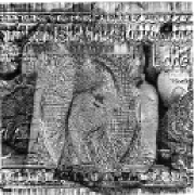
Figure 11: 11 $1$ Degree rotated watermarked image and 11 Extracted watermark.

V.7 Gamma Correction

In general many output devices, say computer displays, have a nonlinear response to that of the input signal. Gamma correction is applied to compensate for this effect. Typically, the response follows a power law; $x^{\gamma}$. In the case of images, a gamma correction to it has the effect of compressing and expanding the pixel value. When $\gamma<1$ it is called compression and for $\gamma>1$ it is called expansion. Since, $\gamma$ is related to the value of the pixel, which in turn directly translates into visual quality of images, a gamma correction leads to brighter or darker images depending on the value of $\gamma$.

Figures 12 and 12 show the watermarked image and the extracted watermark respectively after gamma compression with $\gamma=0.95$. Figures 12 and 12 show the watermarked and extracted images respectively after gamma expansion with $\gamma=1.09$. In both the cases, the extracted watermark is clearly visible and PSNR value is within the acceptable limits.

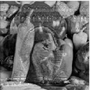
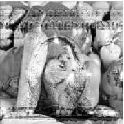
Figure 12: 12, 12 Gamma $0.95$ watermarked image and Extracted watermark 12, 12 Gamma $1.09$ watermarked image and Extracted watermark.

V.8 Intensity Adjustment

Intensity adjustment is a technique of mapping an image’s intensity values to a new range. In the present example, we have mapped the watermarked image’s intensity to the range 0.1-1.0. As shown in Fig. 13 and 13, the watermark recovered from the intensity adjusted image does not suffer much distortion.

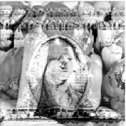
Figure 13: 13 Intensity adjusted watermarked image and 13 Extracted watermark.

V.9 Gaussian Blur

The Gaussian blur filter, as implied by its very name, blurs objects. This filter creates an output image after applying a Gaussian weighted average of the input pixels around the location of each corresponding output pixel. Figure 14 is the Gaussian blurred watermarked image and Fig. 14 is the watermark extracted from it.

Blurring can also be achieved by a simple low-pass filter. Its mainly applied to average out the rapid changes in the intensity of the image. This is achieved by calculating the average of a pixel and all of its eight immediate neighbors. This average is then used instead of the original value of the pixel. This process is repeated for every pixel of the image. Since, this is very similar to the Gaussian blur attack, already presented, we will not give the resulting images of this experiment. Suffice to say that the extraction of the watermark is possible.

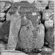
Figure 14: 14 Watermarked image after Gaussian blur and 14 Extracted watermark.

V.10 Contrast Enhancement

Contrast enhancement is the process by which the contrast of an image is modified. This can significantly improve the visual quality of the image. In this process the darker colors are made more dark and the lighter regions more light. This is achieved in the following way. We choose a particular cut off for the darker as well as the lighter regions and all the pixel values that are smaller and larger than this cut off are set to their mnimimum and maximum values respectively. For example, in the case of a greyscale image all pixel values that are smaller than the lower bound, chosen apriori, are made black. Correspondingly all pixel values larger than the chosen upper bound are set to $255$, i.e., made white. The rest of the values that lie in between this minimum and maximum bound are spread linearly on a $0$ to $255$ scale.

The result of this attack on the watermarked image is shown in Fig. 15 and that of the extracted watermark is shown in Fig. 15. The enhancement value chosen in the present case is $0.75$. We have also checked it for another value $1.25$ and from the PSNR and RMSE values given in the table, the quality of the embedded and the extracted watermark actually improves with a higher value of enhancement.

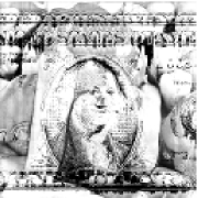
Figure 15: 15 Watermarked image after applying contrast enhancement and 15 Extracted watermark.

V.11 Dilation

Dilation in images can be thought of as a morphological operation. When it is applied to grayscale images, the bright regions that are surrounded by dark regions increase in size, whereas the dark regions having bright regions around it reduce in size. The effect is very prominent at places, in the image, where the intensity changes rapidly. Regions where the intensity is fairly uniform remain largely unaffected except at the edges. Thus the overall effect of this operation is to whiten the whole image. The results are shown in Figs. 16 and 16.

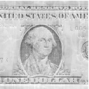
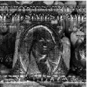
Figure 16: (a) Dilated watermarked image and (b) Extracted watermark.

V.12 Scaling

Scaling operation changes the size of images. This can be of two varieties, namely, uniform and non-uniform. When the horizontal and vertical directions are scaled by the same factor it is called uniform scaling. In contrast to this, non-uniform scaling uses different scaling factors for the horizontal and vertical directions. This latter type of scaling changes the aspect ratio of the image unlike the former. The watermarked and extracted images after uniform scaling are shown in Figs. 17 and 17 respectively. The watermarked image, Fig. 17, and the extracted watermark, Fig. 17, after non-uniform scaling show that our watermarking procedure performs quite well.

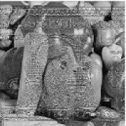
Figure 17: 17, 17 Uniformly rescaled watermarked image and Extracted watermark 17, 17 Non-uniformly rescaled watermarked image and Extracted watermark.

V.13 Image Difference

The absolute difference between the original image and the watermarked image, i.e, Fig. 1 and Fig. 2 is shown in Fig. 18 reveals that the embedded watermark is completely invisible and we only see a corrupted texture of the original image.

Figure 18: Image difference between Fig. 1 and Fig. 2

S.No.	Type of Attack	Software Used	Dollar		Pepper
			PSNR (dB)	RMSE ($\varepsilon$)	PSNR (dB)	RMSE ($\varepsilon$)
$1$.	Tune Sharpen (Directional)	Corel Graphics Suite 11	23.56	16.31	13.19	51.43
$2$.	Smoothing (50%)	Corel Graphics Suite 11	22.53	18.36	10.88	67.14
$3$	Lowpass Blur (Radius 1)	Corel Graphics Suite 11	19.82	25.09	9.30	80.47
$4$	Gaussian Noise	MATLAB R2010a	22.32	18.81	9.83	75.71
$5$.	Gaussian Blur (Radius 1)	Corel Graphics Suite 11	19.18	27.02	8.95	83.85
$6$.	Gamma correction $1.09$	MATLAB R2010a	22.64	18.13	11.59	61.81
$7$.	Gamma correction $0.95$	MATLAB R2010a	24.92	13.94	15.17	40.95
$8$.	Deinterlace (Even line, Interpolation)	Corel Graphics Suite 11	18.87	27.98	11.58	61.92
$9$.	Contrast Enhancement 0.75	Corel Graphics Suite 11	18.59	28.92	7.16	103.04
$10$.	Contrast Enhancement 1.25	Corel Graphics Suite 11	24.00	15.51	8.30	90.32
$11$.	Dilation	GIMP 2.6.10	13.86	49.85	8.28	90.48
$12$.	Erosion	GIMP 2.6.10	12.44	58.73	7.84	95.26
$13$.	Local equalization (80, 80)	Corel Graphics Suite 11	11.90	62.47	6.38	112.61
$14$.	Rotation 1 degree (Bilinear)	MATLAB R2010a	13.18	53.89	7.91	94.48
$15$.	Additive Noise	MATLAB R2010a	18.56	29.01	13.37	50.59
$16$.	Cropping	MATLAB R2010a	11.21	67.66	13.62	48.98
$17$.	Median Filter (3$\times$3)	MATLAB R2010a	18.86	28.04	9.8	75.85
$18$.	Intensity Adjustment	MATLAB R2010a	20.86	22.25	9.52	78.51
$19$.	Uniform Rescaling (512-256-512)	Xn View	19.17	27.05	9.06	82.75
$20$.	Non-uniform Rescaling (512-(320$\times$240)-512)	Xn View	5.78	126.37	9.10	82.38
$21$.	JPEG $20\%$	MATLAB R2010a	20.70	22.67	9.67	77.37
$22$.	JPEG $40\%$	MATLAB R2010a	21.98	19.57	10.47	70.85
$23$.	JPEG $60\%$	MATLAB R2010a	22.76	17.89	11.08	65.61
$24$.	JPEG $80\%$	MATLAB R2010a	23.63	16.18	12.66	54.68
$25$.	JPEG2000 (Compression ratio $2$)	MATLAB R2010a	24.26	15.05	20.23	22.88
$26$.	JPEG2000 (Compression ratio $4$)	MATLAB R2010a	23.92	15.66	13.55	49.33
$27$.	JPEG2000 (Compression ratio $6$)	MATLAB R2010a	23.26	16.88	11.50	62.51
$28$.	JPEG2000 (Compression ratio $8$)	MATLAB R2010a	22.64	18.14	10.50	70.11
$29$.	JPEG2000 (Compression ratio $10$)	MATLAB R2010a	22.07	19.36	10.01	74.17
$30$.	JPEG2000 (Compression ratio $12$)	MATLAB R2010a	21.51	20.65	9.68	77.06
$31$.	JPEG2000 (Compression ratio $14$)	MATLAB R2010a	21.09	21.69	9.42	79.36
$32$.	JPEG2000 (Compression ratio $16$)	MATLAB R2010a	20.72	22.63	9.19	81.56
$33$.	JPEG2000 (Compression ratio $18$)	MATLAB R2010a	20.43	23.40	9.05	82.89
$34$.	JPEG2000 (Compression ratio $20$)	MATLAB R2010a	20.19	24.06	8.93	83.96

Table 1: Table showing different types of attacks performed on the watermarked images. The PSNR and RMSE values of the watermarked as well as the extracted image are given.

VI Summary

In this paper we have introduced a new watermarking scheme based on the Hilbert transform of digital images. Due to inherent ambiguities with the definitions of two-dimensional Hilbert transform, we apply the one-dimensional Hilbert transforms column-wise to any image matrix in which information is sought to be embedded. The Hilbert transformed digital image is defined through its matrix of phase and amplitude values. The main idea behind the proposed technique is that the phase of the analytic signal associated with typical digital images is generally a sparse matrix and hence offers large space for hiding information in a highly imperceptible manner.

We have described embedding and extraction algorithms. The embedding is performed in the Hilbert transformed domain. The Hilbert transform of a watermark image is embedded in the Hilbert transformed domain of the host image, after suitable scaling by a factor $\lambda$. An efficient algorithm for computing the optimal scaling factor $\lambda$ has been derived. The quality of the watermarked image and extracted watermark have been shown to be good when measured in terms of PSNR and RMSE. In addition, we have performed a large number of attacks to study the robustness of our algorithm. The results are summarised in Table (1). The proposed method is shown to be robust against additive noise, cropping, gaussian noise, JPEG/JPEG 2000 compression, median filtering, rotation, gamma correction, intensity adjustment, gaussian blur, contrast enhancement, dilation, rescaling and image difference. We would like to emphasise that calculating Hilbert transforms can be efficiently done on personal computers too. It is not computationally exacting. Thus, we believe that our algorithm can also be modified to suit real-time applications in an efficient manner.

References

- (1) G. Langelaar, I. Setyawan, and R. L. Lagendijk, “Watermarking digital image and video data. A state-of-the-art overview,” IEEE Signal Processing Magazine. 17(5), 20-46 (2000).
- (2) I. J. Cox, M. L. Miller, and J. A. Bloom, Digital watermarking, Morgan Kaufmann Publishers, Inc., San Francisco (2001).
- (3) W. Zeng, “Digital watermarking and data hiding: technologies and applications,” Proc. of ICISAS. 3, 223-229 (1998).
- (4) F. A. P. Petitcolas, R. J. Anderson, and M. G. Kuhn, “Information Hiding: A Survey,” Proc. of the IEEE. 87(7), 1062-1078 (1999).
- (5) S. Craver, N. Memon, B. -L. Yeo, and M. M. Yeung, “Resolving rightful ownerships with invisible watermarking techniques: limitations, attacks, and implications,” IEEE Journal on Selected areas in Communications. 16(4), 573-586 (1998).
- (6) A. Piva, M. Barni, and F. Bartolini, “Copyright protection of digital images by means of frequency domain watermarking,” Proceedings of the Conference on Mathematics of Data/Image Coding, Compression and Encrypyion, SPIE. 3456, 25-34 (1998).
- (7) W. Zeng and B. Liu, “A statistical watermark detection technique without using original images for resolving rightful ownerships of digital images,” IEEE Trans. Image Processing. 8(11), 1534-1548 (1999).
- (8) I. J. Cox, J. Kilian, T. Leighton, and T. Shamoon, “Secure Spread Spectrum Watermarking for Multimedia,” IEEE Transactions on Image Processing. 6(12), 1673-1687 (1997).
- (9) C. I. Podilchuk and E. J. Delp, “Digital Watermarking: Algorithms and Applications,” IEEE Signal Processing Magazine., 18(4), 33-46 (2001).
- (10) M. Kallel, M. S. Bouhlel, and J. C. Lapayre, “A new Multiple Watermarking Scheme for Medical Image in Spatial Field,” GVIP Journal. 7(1), 37-42 (2007).
- (11) M. S. Raval and P. P. Rege, “Scalar Quantization Based Multiple Patterns Data Hiding Technique for Gray Scale Images,” GVIP Journal. 5(9), 55-61 (2005).
- (12) M. Barni, F. Bartolini, V. Cappellini, and A. Piva, “A DCT domain system for robust image watermarking,” IEEE Transactions on Signal Processing. 66(3), 357-372 (1998).
- (13) W. C. Chu, “DCT based image watermarking using subsampling,” IEEE Trans Multimedia. 5, 34-38 (2003).
- (14) J. R. Hernandez, M. Amado, and F. Perez-Gonzalez, “DCT-Domain Watermarking Techniques for Still Images: Detector Performance Analysis And a New Structure,” in IEEE Trans. Image Processing. 9, 55-68 (2000).
- (15) T. B. Dickinson, “Adaptive watermarking in the DCT domain” IEEE ICASSP. 4, 2985 (1997).
- (16) A. Piva, M. Barni, F. Bartolini, and V. Capellini, “DCT-based watermark recovering without resorting to the uncorrupted original image,” IEEE-ICIP. 1, 520-523 (1997).
- (17) D. Kundur and D. Hatzinakos, “A Robust Digital Image Watermarking Scheme using Wavelet-Based fusion,” IEEE - ICIP. 1, 544-547 (1997).
- (18) M. Barni, F. Bartolini, V. Cappellini, and A. Piva, “Improved wavelet based watermarking through pixel-wise masking,” IEEE Trans Image Processing. 10(5), 783-791 (2001).
- (19) Y. Wang, J. F. Doherty, and R. E. Van Dyck, “A wavelet based watermarking algorithm for ownership verification of digital images,” IEEE Transactions on Image Processing. 11(2), 77-88 (2002).
- (20) D. A. Karras, “A Second Order Spread Sprectrum Modulation Scheme for Wavelet Based Low Error Probability Digital Image Watermarking,” ICGST International Journal on Graphics, Vision and Image Processing. 5(3), 19-28 (2005).
- (21) G. S. El-Taweel, H. M. Onsi, M. Samy, and M. G. Darwish, “Secure and Non-Blind Watermarking Scheme for Color Images Based on DWT,” GVIP Journal. 5(4), 1-5 (2005).
- (22) D. Kundur and D. Hatzinakos, “Digital Watermarking using Multiresolution Wavelet Decomposition” IEEE ICASSP. 5, 2969-2972 (1998).
- (23) C. C. Chang, P. Tsai, and C. C. Lin, “SVD based digital image watermarking scheme,” Pattern Recognition Letters. 26, 1577-1586 (2005).
- (24) K. L. Chung, C. H. Shen, and L. C. Chang, “A Novel SVD and VQ-based image hiding scheme,” Pattern Recognition Letters. 22, 1051-1058 (2001).
- (25) R. Liu and T. Tan, “An SVD-based watermarking scheme for protecting rightful ownership,” IEEE Trans. Multimedia. 4(1), 121-128 (2002).
- (26) V. I. Gorodetski, L. J. Popyack, V. Samoilov, and V. A. Skormin, “SVD-based Approach to Transparent Embedding Data into Digital Images,” International Workshop on Mathematical Methods, Models and Architectures for Computer Network Security (MMM-ACNS 2001), St. Petersburg, Russia (2001).
- (27) D. V. S. Chandra, “Digital Image Watermarking Using Singular Value Decomposition,” Proceedings of 45th IEEE Midwest Symposium on Circuits and Systems, 264-267 (2002).
- (28) R. Sun, H. Sun, and T. Yao, “A SVD and quantization based semi-fragile watermarking technique for image authentication,” Proc. IEEE International Conf. Signal Process. 2, 1592-95 (2002).
- (29) Y. Wu, “On the Security of an SVD-Based Ownership Watermarking,” IEEE transactions on Multimedia. 7(4), 624-627 (2005).
- (30) R. Agarwal and M. S. Santhanam, “Digital watermarking using SVD in the singular vector domain, International Journal of Image and Graphics 8, 351-368 (2008).
- (31) J. M. Shieh, D. C. Lou, and M. C. Chang, “A semi-blind digital watermarking scheme based on singular value decomposition,” Computer Standards and Interfaces. 28, 428-440 (2006).
- (32) H. C. Andrews and C. L. Patterson, “Singular value Decomposition (SVD) Image Coding,” IEEE Trans. on communications. 24, 425-432 (1976).
- (33) P. C. Su and C.-C. Jay Kuo, “Spatial-frequency composite watermarking for digital image copyright protection,” Proc. SPIE. 3971, 295 (2000).
- (34) E. Ganic and A. M. Eskiciogulu et. al., “Robust SVD-DCT domain Image Watermarking for copyright Protection: Embedding data in All Frequencies,” 13th European Signal Processing Conference (EUSIPCO 2005) Antalya, Turkey, (2005).
- (35) E. Ganic and A. M. Eskiciogulu, “Robust embedding of Visual Watermarks using discrete wavelet transform and singular value decomposition,” J. Electron. Imaging. 14, 043004 (2005).
- (36) G. Bhatnagar, Q. M. Jonathan Wu, and B. Raman, “SVD-based robust watermarking using fractional cosine transform,” Proc. SPIE 7708, 77080 O (2010).
- (37) H. L. Stefan, Hilbert transforms in signal processing, Artech House Inc., Boston (1996).
- (38) W. B. Pennebaker and J. L. Mitchell, JPEG still image compression standard, Kluwer acadmic publishers group, Dordrecht (2004).
- (39) D. Taubman and M. Marcellin, JPEG2000 image compression fundamentals, standards and practice, Kluwer acadmic publishers group, Dordrecht (2001).