The Effect of the Disorder on the Longitudinal Resistance of a Graphene p-n Junction in Quantum Hall Regime

Abstract

The longitudinal resistances of a six-terminal graphene p-n junction under a perpendicular magnetic field are investigated. Because of the chirality of the Hall edge states, the longitudinal resistances on top and bottom edges of the graphene ribbon are not equal. In the presence of suitable disorder, the top-edge and bottom-edge resistances well show the plateau structures in the both unipolar and bipolar regimes and the plateau values are determined by the Landau filling factors only. These plateau structures are in excellent agreement with the recent experiment. For the unipolar junction, the resistance plateaus emerge in the absence of impurity and they are destroyed by strong disorder. But for the bipolar junction, the resistances are very large without the plateau structures in the clean junction. The disorder can strongly reduce the resistances and leads the formation of the resistance plateaus, due to the mixture of the Hall edge states in virtue of the disorder. In addition, the size effect of the junction on the resistances is studied and some extra resistance plateaus are found in the long graphene junction case. This is explained by the fact that only part of the edge states participate in the full mixing.

I Introduction

The successful fabrication of graphene, a monolayer of carbon atoms arranged hexagonally, sci306-666 ; nat438-197 ; nat438-201 had fueled many experimental and theoretical works. For undoped 2-D graphene sheet, Fermi energy is located at the Dirac neutral point. Around the Dirac point, the graphene has a linear dispersion relation, which leads to quasiparticles obeying the massless Dirac-like equation and presents extraordinary properties.rmp81-109 ; rmp80-1337 ; prb53-2449 For example, for a graphene under a strong perpendicular magnetic field, its Hall plateaus assume half-integer values,nat438-197 ; nat438-201 ; natmat6-183 $h/[g(n+1/2)e^{2}]$, where $g=4$ is the spin and valley degeneracy and $n$ an integer. By varying the gate voltage, both carrier type and concentration of the graphene sheet can be tuned.prl98-236803 A graphene p-n junction is formed by connecting up one p-type graphene and one n-type graphene. Many exciting phenomena closely related to the massless Dirac character of carriers,natphys2-620 ; prl102-026807 ; sci315-1252 ; natphy3-172 ; natphy3-192 such as relativistic Klein tunneling natphys2-620 ; prl102-026807 and Veselago lensing sci315-1252 , are predicted for graphene p-n junctions.

Recently, the electron transport through the graphene p-n or p-n-p junctions was extensively investigated both experimentally and theoretically.sci317-638 ; nanolett9-1973 ; prl99-166804 ; prb79-195327 ; sci317-641 In quantum Hall regime, Williams et al. sci317-638 experimentally found that the two-terminal conductance exhibits plateaus with half-integer values, $g(|n|+1/2)e^{2}/h$, in the case of unipolar junctions and fractional values for bipolar junctions. At about the same time, the theoretical works by Abanin and Levitov sci317-641 explained the appearance of the fractional plateaus by means of the mixture of the electron-like and hole-like Hall edge states in the vicinity of the junction boundary. There were some subsequent investigations on graphene junctions. Using Anderson short-range disorder potentials, Long et al. prl101-166806 and Li et al. prb78-205308 numerically computed and analysed the transport behavior of graphene junctions. They found that conductance plateaus emerge in the case of suitable disorder strength. Also, T. Low prb80-205423 considered the long-range interface and edge disorders in the armchair, zigzag, and antizigzag edge graphene ribbons, and numerically simulated the result of the conductance plateaus.

Very recently, Lohmann et al. nanolett9-1973 measured the Hall and longitudinal resistances in a six-terminal graphene junction device. In their experiment, the difference of carrier concentrations between two adjacent regions (the left and right regions) is introduced by chemical doping, and a global gate voltage controls the carrier concentrations in the two regions. By tuning the gate voltage and doping densities, the graphene ribbon can be of p-p, p-n, n-p, or n-n type. They found that Hall resistances of the left and right regions exhibit half-integer plateaus, as usual. Furthermore, the longitudinal resistances also exhibit plateau structures. In particular, the longitudinal resistances at opposite edges are not equal. For instance, with the filling factors $(\nu_{L},\nu_{R})=(2,-2)$ (here $\nu_{L/R}$ is the Landau filling factor in the left/right region), the longitudinal resistance at one edge is $h/e^{2}$ but it is zero at the other edge. By using the concept of the mixture of Hall edge states near the p-n junction boundary, they explained the appearance of these plateaus and the difference between the longitudinal resistances at the opposite edges. So far, there is not any theoretical investigation which gives quantitative and numerical result to explain Lohmann’s experimental result. More effort needs to be done in order to find out how disorders affect the resistance plateaus and how the plateaus depend on disorder strength.

In this paper, we theoretically and numerically study electron transport through graphene junctions. Following the experiment by Lohmann et al., we consider the six-terminal graphene junction device [shown in Fig. 1(a)]. A perpendicular magnetic field $B$ is applied to the graphene sheet. By using the tight-binding Hamiltonian and the Landauer-Büttiker formulism in the framework of non-equilibrium Green’s function method, the longitudinal and Hall resistances are calculated. The numerical results show that the longitudinal resistances $R_{t}$ and $R_{b}$ of the top and bottom edges, respectively, are usually different in the presence of the magnetic field, as expected from the property of the chirality of Hall edge states. There is an essential difference in the transport behavior between unipolar and bipolar graphene junctions. For unipolar (n-n and p-p) junctions, the longitudinal resistances have plateau structures in the case of clean (no disorder) graphene. The resistance plateaus can keep in the moderate disorder strength, and they are destroyed until the very strong disorder. On the other hand, for bipolar (n-p and p-n) graphene junctions, the longitudinal resistances $R_{t}$ and $R_{b}$ are very large in the clean case. But in the presence of disorder, they are strongly decreased even when the disorder strength is weak. For n-p junctions, the top-edge resistance $R_{t}$ reduces to a moderate positive value, but the bottom-edge resistance $R_{b}$ drops to zero or even turns negative. In a suitable range of disorder strength, the resistances $R_{t}$ and $R_{b}$ of bipolar junctions also have plateau structures due to the full mixing of Hall edge states. For the lowest filling factors, the resistance plateaus exist in a very broad range of disorder strength. Hence, they are produced easily in experiment. But for high filling factors, the plateau only emerges in a narrow disorder range, if it exists. Furthermore, for moderate disorder, the plots of the longitudinal resistances versus the gate voltage exhibit plateau structures in both cases of unipolar and bipolar junctions and the plateau values are only determined by the filling factors $(\nu_{L},\nu_{R})$, which are in excellent agreement with the recent experiment by Lohmann et al.. In addition, we also find some extra resistance plateaus in long graphene junctions. This is explained by the suggestion that only part of edge states participate in the mixing mechanism.

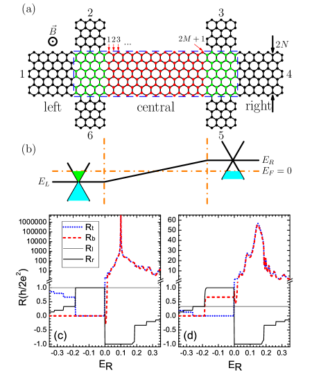
Figure 1: (Color online) The panel (a) is the schematic diagram for the six-terminal graphene p-n junction device and the panel (b) is for the Dirac energy $\epsilon_{i}$ in the left, central and right regions. The panels (c) and (d) show the resistances vs. $E_{R}$ at the clean graphene junction ($W=0$) with $E_{L}=-0.1$ (c) and $-0.2$ (d) , respectively. The other parameters are the width $N=50$, the length $M=20$, and $\phi=0.01$.

The rest of the paper is organized as follows. In Section II, we describe the model and give the details of our calculations. In Section III, the numerical results are given. Finally, a brief conclusion is presented in Section IV.

II Model and calculation

We consider the six-terminal graphene junction device which is illustrated in Fig. 1(a). The six terminals are labelled by the terminal-$i$ ($i=1,2,...,6$). Terminals 1 and 4 are the current source and drain, respectively, and other terminals are used as the voltage probes. The whole graphene device is basically divided into three regions: the left, central and right regions as shown in Fig. 1(a). Each of the left and right regions includes three terminals. The dimension of the central region is described by the integers $N$ and $M$ [see the red-site (dark gray) region in Fig. 1(a)]. There are totally $2N\times(2M+1)$ carbon atoms in the central region. The width and length of the central region are $a(3N-1)$ and $\sqrt{3}a(M+1)$, respectively. The width of voltage terminals is chosen as $\sqrt{3}aN$, where $a\approx 0.142$ nm is the distance between two neighboring carbons. Fig. 1(a) shows the case $N=3$ and $M=10$.

The whole system is subjected to a perpendicular magnetic field which leads to the formation of Landau levels. In quantum Hall regime, bulk states are compressible, and the chiral edge states flow along the edges. This behavior is independent of the type of the edges if the graphene ribbon is wide enough. So we choose wide zigzag-graphene ribbon for our simulation. Compared to the hopping term, both Zeeman splitting and spin-orbit coupling are very small and hence they are negligible. Furthermore, we adopt Anderson on-site disorder. In fact, other types of disorders (e.g. the interface disorder and the long-range disorder) may exist in the experimental device and also lead to the edge state mixing. But from the point of the edge state mixing, these other types of disorders should have the similar effect. Here we can assume Anderson disorder only exists in the central region based on the fact that the effect of disorder in the left and right regions is suppressed by edge states when the ribbon is wide enough.note1

In the tight-binding representation, the Hamiltonian of the six-terminal graphene junction is given byprl101-166806 ; prb78-205308 ; prb73-233406

$$H=\sum_{i}{\epsilon_{i}a_{i}^{\dagger}a_{i}}-\sum_{<ij>}{(te^{i\phi_{ij}}a_{i}^{\dagger}a_{j}+\emph{h.c.})},$$ (1)

where $a_{i}^{\dagger}$ and $a_{i}$ are respectively the creation and annihilation operators at site $i$, and $\epsilon_{i}$ the energy of Dirac point (i.e., the on-site energy). In the left and right regions, $\epsilon_{i}$ is equal to $E_{L}$ and $E_{R},$ respectively [Fig. 1(b)], which can be controlled by the gate voltage in the experiment. In the central region, $\epsilon_{i}=k(E_{R}-E_{L})/(2M+2)+E_{L}+w_{i}$, where the column index $k=1,2,...,2M+1$ [see Fig. 1(a)] and $w_{i}$ is the on-site disorder energy. $w_{i}$ is assumed to be randomly distributed in the range $[-W/2,W/2],$ where $W$ is the disorder strength. The second term in the Hamiltonian stands for the nearest-neighbor hopping. The effect of the magnetic field $B$ is addressed by the phase $\phi_{ij}=\int_{i}^{j}\vec{A}\cdot d\vec{l}/\phi_{0}$ in the hopping interaction Hamiltonian where $\vec{A}=(-By,0,0)$ is the vector potential and $\phi_{0}=\hbar/e$. The magnetic field $B$ is applied to the whole device (including the six terminals and central region) along the perpendicular direction.

The multi-terminal resistance prb38-9375 is defined as $R_{ij,kl}=(V_{k}-V_{l})/I_{i\leftarrow j}$, where the contacts $i$ and $j$ are terminals used to draw and input current, and the two contacts $k$ and $l$ are used to measure the voltage difference. We introduce two longitudinal resistances $R_{t}=R_{14,23}$ (on the top edge) and $R_{b}=R_{14,65}$ (on the bottom edge) and two Hall resistances $R_{l}=R_{14,26}$ (in the left region) and $R_{r}=R_{14,35}$ (in the right region). These four resistances obey the relation,

$$R_{t}+R_{r}=R_{b}+R_{l}.$$ (2)

From the Landauer-Büttiker formula at zero temperature, the current flowing into terminal-$i$ is given by $I_{i}=(2e^{2}/h)\sum_{j(\neq i)}T_{ij}(E_{F})(V_{i}-V_{j})$.datta Here, $T_{ij}(E_{F})=\text{Tr}[\mathbf{\Gamma}_{i}\mathbf{G^{r}\Gamma}_{j}\mathbf{G^{a}}]$ $(i,j=1,2,...,6$ and $i\neq j)$ is the transmission coefficient from terminal-$j$ to terminal-$i$ at Fermi energy $E_{F}$, $\mathbf{\Gamma}_{i}(E_{F})=i{[\mathbf{\Sigma}_{i}^{r}(E_{F})-\mathbf{\Sigma}_{i}^{a}(E_{F})]}$ the line width functions, $\mathbf{G}^{r}(E_{F})=[\mathbf{G}^{a}]^{\dagger}=1/[E_{F}-\mathbf{H}_{cc}-\sum_{i=1}^{6}\mathbf{\Sigma}_{i}^{r}]$ the retarded and advanced Greens functions, and $\mathbf{H}_{cc}$ the Hamiltonian of the dashed-box region which includes two green-site (light gray) regions and the red-site (dark gray) central region [see Fig. 1(a)]. The retarded self-energy ${\mathbf{\Sigma}}_{i}^{r}(E_{F})$ due to the coupling to the terminal-$i$ can be calculated numerically.jpf15-851 To determine the longitudinal and Hall resistances mentioned above, we applied a bias $V$ across terminal-1 and terminal-4, and the currents in the voltage probes (terminals 2, 3, 5, and 6) are set to zero. Then from the Landauer-Büttiker formula, the voltages $V_{2}$, $V_{3}$, $V_{5}$ and $V_{6}$ of the voltage probes and the currents $I_{1}$ and $I_{4}$ can be calculated. We should have $I_{1}=-I_{4}\equiv I_{14}$. Finally, the longitudinal and Hall resistances are given by $R_{t}\equiv(V_{2}-V_{3})/I_{14}$, $R_{b}\equiv(V_{6}-V_{5})/I_{14}$, $R_{l}\equiv(V_{2}-V_{6})/I_{14}$ and $R_{r}\equiv(V_{3}-V_{5})/I_{14}$.

The recursive Green’s function technique jpf15-851 is used for the computation of the transmission coefficient. The Fermi energy $E_{F}$ is set equal to zero as the energy reference point. The hopping energy $t\approx$ 2.75 eV is used as the energy unit, which corresponds to $3\times 10^{4}$ K. It is reasonable to assume zero temperature condition in our calculations because the temperature in the experiment is only of several Kelvin or sub-Kelvin. Taking into account the spin degeneracy, we will use $h/2e^{2}$ as the resistance unit. The corresponding filling factors $\nu_{L}$ and $\nu_{R}$ are taken as odd integers ( $\pm 1,\pm 3,\pm 5,...)$ instead of even integers ($\pm 2,\pm 6,\pm 10,...)$. The effect of the constant magnetic field is addressed by appropriate Peierls phase prb77-115408 : $2\phi\equiv(3\sqrt{3}/2)a^{2}B/\phi_{0}$, where $a\approx 0.142$ nm is the distance between two neighboring carbons. We will take $\phi=0.01$ which corresponds to the magnetic length $l_{B}=\sqrt{\hbar/(eB)}\approx 1.6$ nm.note2 We will consider the case $N=50$ and $M=20$, where the area of the central region is $21.2\times 5.2$ nm² and the width of the voltage terminals is $12.3$ nm. The reason for using a width of the graphene ribbon far larger than the magnetic length is that edge states can not mix except near the boundary of the junction. Finally, the disorder is averaged over 2000 random configurations except in Fig. 4(a) and (b), where 500 configurations are taken.

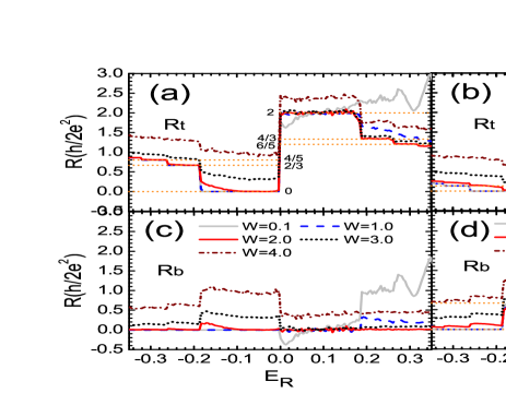
Figure 2: (Color online) The longitudinal resistances $R_{t}$ and $R_{b}$ vs. $E_{R}$ for the different disorder strength $W$ at the energy $E_{L}=-0.1$ [panels (a) and (c)] and $-0.2$ [panels (b) and (d)]. The panels (a) and (b) are for $R_{t}$ and the panels (c) and (d) are for $R_{b}$. The other parameters are the same as in Fig. 1(c) and (d).

III Numerical results and analysis

We first study the resistances in the clean graphene junction under a strong magnetic field with $\phi=0.01$. In Fig. 1 (c) and (d), the Hall and longitudinal resistances ($R_{l}$, $R_{r}$, $R_{t}$, and $R_{b}$) versus the Dirac energy $E_{R}$ of the right region are shown. The Dirac energy $E_{L}$ of the left region is fixed at $-0.1$ [Fig. 1(c)] or $-0.2$ [Fig. 1(d)], which corresponds to $\nu_{L}=1$ and $3$, respectively. As usual, the Hall resistances $R_{l}$ and $R_{r}$ display quantized plateaus with plateau values $\pm 1,~{}\pm 1/3,~{}\pm 1/5,$ … [in units of $h/2e^{2}$], and Hall plateau of a region only depends on the filling factor of the region, $R_{l}=1/\nu_{L}$ and $R_{r}=1/\nu_{R}$. Furthermore, the Hall resistance plateaus are found to be unaffected by the sizes of the central region and the presence of the disorder in the central region, because that the Hall effect is very robust. We will then focus our study on the longitudinal resistances $R_{t}$ and $R_{b}$.

In the presence of the magnetic field, the longitudinal resistance $R_{t}$ of the top edge usually is not equal to $R_{b}$ of the bottom edge regardless of the junction type and disorder strength $W$, because Hall edge states have the chirality which breaks the symmetry of the top and bottom edges. With $E_{R}<0$, both $R_{t}$ and $R_{b}$ of the clean n-n junction device exhibit perfect plateau structures [Fig. 1(c) and (d)]. By considering the carrier transport along the edges, the plateau values can be analytically obtained:

$$R_{t}=\left(\frac{1}{|\nu_{L}|}-\frac{1}{|\nu_{R}|}\right)\frac{h}{2e^{2}}\quad\mathrm{\ and}\quad R_{b}=0$$ (3)

for the n-n⁺ regime ($0<\nu_{L}\leq\nu_{R}$) and

$$R_{t}=0\quad\mathrm{\ and}\quad R_{b}=\left(\frac{1}{|\nu_{R}|}-\frac{1}{|\nu_{L}|}\right)\frac{h}{2e^{2}}$$ (4)

for the n⁺-n regime ($0<\nu_{R}\leq\nu_{L}$). The plateau values can be understood from the following simple argument. It is well known that, for the n-n regime the carriers are electron-like and they move clockwise. For the case $0<\nu_{L}\leq\nu_{R}$ (the n-n⁺ regime), all edge states at the bottom edge are from the right reservoir (i.e. terminal-4), so the voltages $V_{6},V_{5}$ and $V_{4}$ are all equal and this leads to $R_{b}=(V_{6}-V_{5})/I_{14}=0$. According to Eq. (2), $R_{t}$ is then equal to $(1/|\nu_{L}|-1/|\nu_{R}|)h/2e^{2}$. The numerical results in Fig. 1(c) and (d) are consistent with the plateau values given in Eqs.(3) and (4). For example, in Fig. 1(c) where $\nu_{L}=1$, the resistance $R_{b}$ is zero and $R_{t}$ can be equal to $0$, $(2/3)h/2e^{2}$, $(4/5)h/2e^{2}$, … for $\nu_{R}=1$, $3$, $5$, …. And in Fig. 1(d) where $\nu_{L}=3$, $R_{b}$ is $0$ or $(2/3)h/2e^{2}$ and $R_{t}$ can be $0$, $(2/15)h/2e^{2}$, $(4/21)h/2e^{2}$, and so on.

When $E_{R}>0$ the device becomes a n-p junction. There is no plateau structure for $R_{t}$ and $R_{b}$, according to Fig. 1(c) and (d). Both $R_{t}$ and $R_{b}$ are very large and they are almost equal. Furthermore, the smaller the filling factors are, the larger the longitudinal resistances are. For some values of $E_{R}$, $R_{t}$ and $R_{b}$ can be over $1000h/2e^{2}$ (about $13M\Omega$). This is because for the case of clean n-p junction, the edge states in the left and right regions have different chiralities and they are well separated in space. Hence, edge states mixture can not occur and this leads to very large longitudinal resistances.

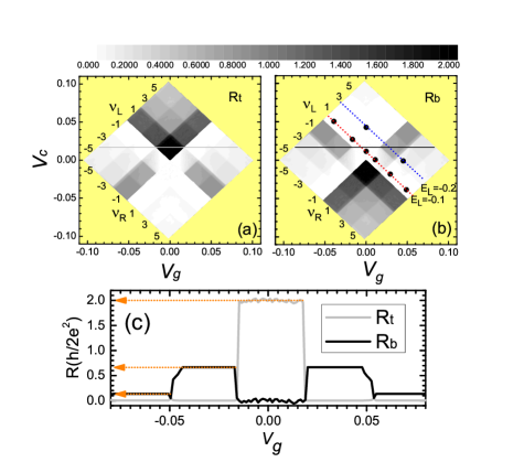
Figure 3: (Color online) The 2-D plots of the longitudinal resistance $R_{t}$ (a) and $R_{b}$ (b) as a function of $V_{g}$ and $V_{c}$, with the parameters $N=50$, $M=20$, $W=2$ and $\phi=0.01$. (c) The one-dimensional slices shown in (a) (gray solid) and (b) (black solid) are plotted to show the dependence of $R_{t}$ and $R_{b}$ on $V_{g}$ with $V_{c}$ fixed at 0.015 and $W=1$.

Next, we shall discuss how $R_{t}$ and $R_{b}$ are affected by disorder. Fig. 2 shows the dependence of $R_{t}$ and $R_{b}$ on the Dirac energy $E_{R}$ for different disorder strength $W$. $E_{L}$ is fixed at $-0.1$ ($\nu_{L}=1$) or $-0.2$ ($\nu_{L}=3$). For n-n regime ($E_{R}<0$), the plateau structures of $R_{t}$ and $R_{b}$ still exist for weak and moderate disorder strength. And the plateau values are the same as that of the clean graphene junction. However, in the case of strong disorder (e.g. $W>3$), $R_{t}$ and $R_{b}$ increase and the plateau structures disappear. This is expected as Hall edge states begin to be destroyed by strong disorder. For n-p regime ($E_{R}>0$), $R_{t}$ and $R_{b}$ are strongly reduced even when the disorder is weak. For example, when $W=0.1$ (very weak) $R_{t}$ and $R_{b}$ are smaller than $3h/2e^{2}$ for any $E_{R}$ (Fig. 2), though $R_{t}$ and $R_{b}$ can be over $1000h/2e^{2}$ at some values of $E_{R}$ for clean junction [Fig. 1(c)]. This significant decrease results from that the electron-like and hole-like Hall edge states start to mix in the vicinity of the n-p interface. It should be obvious from our numerical result that the top-edge and bottom-edge resistances $R_{t}$ and $R_{b}$ are not equal and $R_{b}$ can be negative at some specific values of the parameters [Fig. 2(c)]. For suitable disorder strength, the full edge-state mixture occurs and hence $R_{t}$ and $R_{b}$ exhibit plateau structures (see the curves of $W=2$ in Fig. 2). According to the Landauer-Büttiker formula under the condition of full edge-state mixture in the central region (junction), the plateau values can be analytically obtained:

$$R_{t}=(\frac{1}{|\nu_{L}|}+\frac{1}{|\nu_{R}|})\frac{h}{2e^{2}}\mathrm{\quad and\quad}R_{b}=0.$$ (5)

In Fig. 2, the plateau values for some low filling factors $(\nu_{L},\nu_{R})$ have been labeled and they are well consistent with the numerical results.

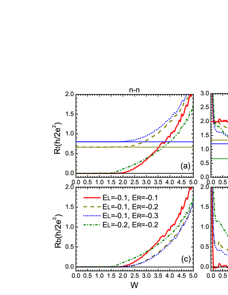
Figure 4: (Color online) The disorder dependence of longitudinal resistances $R_{t}$ and $R_{b}$ with selected $(\nu_{L},\nu_{R})$ [which are represented by the solid dots in Fig. 3(b)]. (a) and (b) are for $R_{t}$ and (c) and (d) are for $R_{b}$. The other parameters are the same as in Fig. 1(c).

In the following we shall base on our model to simulate the recent experimental results. In Ref. nanolett9-1973, , a difference of carrier concentrations between the left and right regions was introduced by chemical doping and a global gate voltage $V_{g}$ was used to control the carrier concentrations of the whole region. So in our theoretical work, we instead introduce two voltages $V_{g}$ and $V_{c}$ to control the carrier concentrations. Let $n_{L/R}$ be the carrier concentration in the left/right region. $n_{L}$ and $n_{R}$ are related to $V_{g}$ and $V_{c}$ in the following way: $n_{L}\propto-V_{g}-V_{c}$ and $n_{R}\propto-V_{g}+V_{c}$. Because of the linear dispersion relation of graphene, the carrier concentration $n_{L/R}$ is approximatively proportional to $\mathrm{sgn}(E_{L/R})E_{L/R}^{2}$.nanaores1-361 ; note3 So we have

$$\mathrm{sgn}(E_{L})E_{L}^{2}=\beta(-V_{g}-V_{c}),\mathrm{sgn}(E_{R})E_{R}^{2}=\beta(-V_{g}+V_{c}),$$ (6)

where $\beta$ is a constant. We assign $\beta$ to be 1 in order to simplify the expressions.

Figs. 3(a) and (b) are the 2-D plots of $R_{t}$ and $R_{b}$ as functions of $V_{g}$ and $V_{c}$ with the disorder strength $W=2$. The axes $E_{L}$ (or $\nu_{L}$) and $E_{R}$ (or $\nu_{R}$) shown in Figs. 3(a) and 3(b) are determined by Eq.(6). The dotted lines in Fig. 3(b) are identical to the curves plotted in Fig. 2. From the figure we see that $R_{t}$ and $R_{b}$ have the following symmetry properties: (i) a mirror symmetry with respect to the line $V_{g}=0$

$$R_{t}(\nu_{L},\nu_{R}) = R_{t}(-\nu_{R},-\nu_{L})$$ (7)

$$R_{b}(\nu_{L},\nu_{R}) = R_{b}(-\nu_{R},-\nu_{L}),$$ (8)

which reflects the inversion of the edge-state chiralities; (ii) an inversion symmetry

$$R_{t}(\nu_{L},\nu_{R})=R_{b}(\nu_{R},\nu_{L})$$ (9)

because of the interchange of $R_{t}$ and $R_{b}$ by rotating the angle $\pi$ round the center of the device. Furthermore, both resistances $R_{t}$ and $R_{b}$ exhibit the plateaus in the whole space of the parameters $V_{g}$ and $V_{c}$. $R_{t}$ and $R_{b}$ are approximatively constants at fixed filling factors $(\nu_{L},\nu_{R})$. But as $(\nu_{L},\nu_{R})$ varies, the jump of $R_{t}$ and $R_{b}$ occurs so that the borders of the filling factors $(\nu_{L},\nu_{R})$ are clearly seen in Fig. 3(a) and (b). Here the resistance plateau values in n-n and n-p regimes are coincidental with Eqs.(3), (4) and (5).

In Fig. 3(c), the variations of $R_{t}$ and $R_{b}$ along the horizontal solid lines in Fig. 3(a) and (b) are shown. With the range of the gate voltage $V_{g}$ from $-0.1$ to $0.1$, the corresponding filling factors $(\nu_{L},\nu_{R})$ are $(-3,-5)$, $(-1,-3)$, $(1,-1)$, $(3,1)$, and $(5,3)$. The figure shows that in unipolar (n-n and p-p) regime, the top-edge resistance $R_{t}$ is always equal to zero. But the bottom-edge resistance $R_{b}$ is $(2/3)h/2e^{2}$ at $(\nu_{L},\nu_{R})=(-1,-3)$ and $(3,1)$, and $(2/15)h/2e^{2}$ at $(\nu_{L},\nu_{R})=(-3,-5)$ and $(5,3)$. For the bipolar (n-p) regime, $(\nu_{L},\nu_{R})=(1,-1)$, the plateau of $R_{t}$ is $2h/2e^{2}$ and $R_{b}$ is zero. These resistance plateau values are well in agreement with the recent experiment results [see Fig.5(c) in Ref. nanolett9-1973, ].

The disorder strength dependence of the longitudinal resistances at the selected filling factors $(\nu_{L},\nu_{R})$ from Fig. 3(b) (represented by solid dots) is shown in Fig. 4. Because of the relation between $R_{t}$ and $R_{b}$ given in Eq. (2), $R_{t}$ and $R_{b}$ have similar characteristics with respect to the disorder strength $W$ even though $R_{t}\not=R_{b}$. For n-n regime (see the left panels of Fig. 4), $R_{t}$ and $R_{b}$ in the clean junction ($W=0$) have plateau structure. The plateau structure still exists when $W$ increases from zero. However, when $W$ increases beyond a critical value $W_{c}$, $R_{t}$ and $R_{b}$ start to increase from the plateau values. The critical value $W_{c}$ is found to be dependent on the filling factors $(\nu_{L},\nu_{R})$: $W_{c}\approx 2.0$ for $(\nu_{L},\nu_{R})=(1,1)$, $(1,3)$ and $(1,5)$, and $W_{c}\approx 1.5$ for $(\nu_{L},\nu_{R})=(3,3)$. However, for n-p regime (see the right panels of Fig. 4), $R_{t}$ and $R_{b}$ are very large in the clean junction. When $W$ increase from zero, $R_{t}$ and $R_{b}$ decrease sharply. For example, when $W$ increases from zero to 0.1, $R_{t}$ is reduced by two or three orders of magnitude to a finite value, while $R_{b}$ is reduced to zero. As $W$ continues to increase, both $R_{t}$ and $R_{b}$ decrease to certain plateau values. The plateau exists in a certain range of disorder strength, where the full mixing of the electron-like and hole-like edge state occurs. For the lowest filling factors $(\nu_{L},\nu_{R})=(1,-1)$, the plateau values $R_{t}=h/e^{2}$ and $R_{b}=0$ exist in a very broad range of disorder strength, from $0.1$ to $3.0$. For $(\nu_{L},\nu_{R})=(1,-3)$ and $(1,-5)$, the disorder range for the existence of resistance plateau are from 1.7 to 2.7 and from 1.9 to 2.7, respectively, which is narrower than that of $(1,-1)$. For higher filling factors [$(\nu_{L},\nu_{R})=(3,-3)$ or higher], the plateau does not exist, due to the fact that it is more difficult to completely mix all edge states in the case of high filling factors. This means that the resistance plateaus with lower filling factors are easier to be observed in experiment. Finally, when $W$ further increase to be large than 3, $R_{t}$ and $R_{b}$ start to increase for all cases of filling factors, which indicates that the edge states are destroyed by strong disorder.

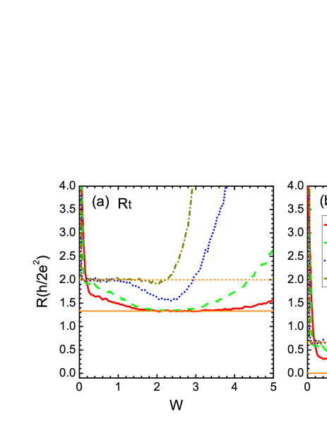
Figure 5: (Color online) The resistances $R_{t}$ (a) and $R_{b}$ (b) vs. the disorder strength $W$ for the different length $M$ of the center region. The parameters are $E_{L}=-0.1$, $E_{R}=0.2$, $\phi=0.01$, and $N=50$.

Now we study the size effect of the central region on $R_{t}$ and $R_{b}$. For unipolar graphene junction, the resistances $R_{t}$ and $R_{b}$ are almost unaffected by the length $M$ and width $N$ of central region, except for the case of very small $N$. In the following we focus on the bipolar junction case. Fig. 5 shows the dependence of $R_{t}$ and $R_{b}$ on disorder strength $W$ at different length $M$ for the filling factors $(\nu_{L},\nu_{R})=(1,-3)$. For other filling factors, the results are similar. From Fig. 5, we can see that when the central region is short (e.g. $M=10$), the full-mixing ideal plateaus [$R_{t}=(4/3)h/2e^{2}$ and $R_{b}=0$] exist in a wide disorder range $1.6<W<4$. This can be understood as the small size of the central region makes the edge states close to each other and hence the full mixing of the states occurs. With increasing length $M$, the full mixing is more difficult. Under this condition $R_{t}$ and $R_{b}$ are enhanced and the corresponding disorder range for the ideal plateaus narrows down or even disappears. For example, for $M=20$, the ideal plateau exists only in the disorder range $1.7<W<2.7$ which is much narrower than that of $M=10$. For larger $M$ such as $50$ and $100$, the ideal plateaus do not exist in any case of disorder strength. Although full-mixing plateaus disappear in the case of longer junction, extra plateaus [$R_{t}=2h/2e^{2}$ and $R_{b}=(2/3)h/2e^{2}$] emerge in a long enough junction (e.g. $M=100$). The existence of the extra plateaus can be explained by the partial mixing of edge states. The assumption of partial mixing of edge states in long enough junctions is reasonable, because part of the Hall edge states are near the junction boundary but the other Hall edge states are far away from the boundary. Let us assume that there are $(x_{L},x_{R})$ edge states taking part in the full mixing [i.e., the residual $(|\nu_{L}|-x_{L},|\nu_{R}|-x_{R})$ edge states in the left and right regions do not participate in any mixing], the plateau values can be analytically obtained by Landauer-Büttiker formalism:

$$R_{t} = (\frac{1}{x_{L}}+\frac{1}{x_{R}})\frac{h}{2e^{2}}$$

$$R_{b} = (\frac{1}{x_{L}}+\frac{1}{x_{R}}-\frac{1}{|\nu_{L}|}-\frac{1}{|\nu_{R}|})\frac{h}{2e^{2}}$$ (10)

If $x_{L}=|\nu_{L}|$ and $x_{R}=|\nu_{R}|$ (i.e. full mixing), the result of Eq.(III) reduces to Eq.(5). By taking $x_{L}=1$, $x_{R}=1$ and $(\nu_{L},\nu_{R})=(1,-3)$, the plateau values given by Eq.(III) are $R_{t}=2h/2e^{2}$ and $R_{b}=(2/3)h/2e^{2}$, which are well consistent with the numerical results in Fig. 5.

Finally, we simply discuss how the width $N$ of a graphene junction affects $R_{t}$ and $R_{b}$. With increasing $N$ at fixed length $M$, the resistances $R_{t}$ and $R_{b}$ decrease, the resistance plateaus exist in broader disorder range regardless of the type of the junction (unipolar or bipolar). Also, for the large $N$, some high-filling-factors resistance plateaus emerge. This is expected as Hall edge states in a wider junction have more chance to mix with each other.

IV Conclusion

In summary, we have investigated the longitudinal resistances at the two edges of a six-terminal graphene junction in the presence of a perpendicular magnetic field. By considering the presence of disorder in the vicinity of the junction interface, the longitudinal resistances at opposite edges exhibit different plateaus structures. It is found that the plateau values are only determined by the Landau filling factors. The numerical results are in excellent agreement with the recent experiment by Lohmann et al.. Furthermore, for unipolar junctions, resistance plateaus exist in clean junctions. The plateau structure can be kept in the presence of weak and moderate disorder, and they are destroyed by very strong disorder. However, for bipolar junctions, the longitudinal resistances are very large and do not have any plateau structure in the clean case. In the presence of disorder, the resistances sharply drop even in the case of very weak disorder and they exhibit plateau structures for suitable disorder strength. In addition, we study the effect of the size of a graphene junction on the resistances and find that some extra resistance plateaus emerge in long graphene junctions. We explain this by proposing that only part of edge states participate in the mixing.

References

- (1) Email address: sunqf@aphy.iphy.ac.cn
- (2) K. S. Novoselov, A. K. Geim, S. V. Morozov, D. Jiang, Y. Zhang, S. V. Dubonos, I. V. Grigorieva, and A. A. Firsov, Science 306, 666 (2004).
- (3) K. S. Novoselov, A. K. Geim, S. V. Morozov, D. Jiang, M. I. Katsnelson, I. V. Grigorieva, S. V. Dubonos, and A. A. Firsov, Nature (London) 438, 197 (2005).
- (4) Y. Zhang, Y.-W. Tan, H. L. Stormer, and P. Kim, Nature (London) 438, 201 (2005).
- (5) A. H. Castro Neto, F. Guinea, N. M. R. Peres, K. S. Novoselov, and A. K. Geim, Rev. Mod. Phys. 81, 109 (2009).
- (6) C.W.J. Beenakker, Rev. Mod. Phys. 80, 1337 (2008).
- (7) G. W. Semenoff, Phys. Rev. Lett. 53, 2449 (1984).
- (8) A. K. Geim and K. S. Novoselov, Nature Mat. 6, 183 (2007).
- (9) B. Huard, J. A. Sulpizio, N. Stander, K. Todd, B. Yang, and D. Goldhaber-Gordon, Phys. Rev. Lett. 98, 236803 (2007).
- (10) M. I. Katsnelson, K. S. Novoselov, and A. K. Geim, Nature Phys. 2, 620 (2006).
- (11) N. Stander, B. Huard, and D. Goldhaber-Gordon, Phys. Rev. Lett. 102, 026807 (2009).
- (12) V. V. Cheianov, V. Fal’ko, and B. L. Altshuler, Science 315, 1252 (2007).
- (13) A. Rycerz, J. Tworzydło, and C. W. J. Beenakker, Nature Phys. 3, 172 (2007).
- (14) B. Trauzettel, D. V. Bulaev, D. Loss, and G. Burkard, Nature Phys. 3, 192 (2007).
- (15) B. Özyilmaz, P. Jarillo-Herrero, D. Efetov, D. A. Abanin, L. S. Levitov, and P. Kim, Phys. Rev. Lett. 99, 166804 (2007).
- (16) D.-K. Ki and H.-J. Lee, Phys. Rev. B 79, 195327 (2009).
- (17) T. Lohmann, K. v. Klitzing, and J. H. Smet, Nano Lett. 9, 1973 (2009).
- (18) J. R. Williams, L. DiCarlo, and C. M. Marcus, Science 317, 638 (2007).
- (19) D. A. Abanin and L. S. Levitov, Science 317, 641 (2007).
- (20) W. Long, Q.-f. Sun, and J. Wang, Phys. Rev. Lett. 101, 166806 (2008).
- (21) J. Li and S.-Q. Shen, Phys. Rev. B 78, 205308 (2008).
- (22) T. Low, Phys. Rev. B 80, 205423 (2009).
- (23) If the disorder region is extended to the whole dashed-box region, including the red-site (dark gray) central region and two green-site (light gray) regions as shown in Fig. 1(a), the numerical results are almost unchanged. This is because the Hall edge states are robust against the disorder.
- (24) D. N. Sheng, L. Sheng, and Z. Y. Weng, Phys. Rev. B 73, 233406 (2006).
- (25) M. Büttiker, Phys. Rev. B 38, 9375 (1988).
- (26) S. Datta, Electronic transport in Mesoscopic Systems (Cambridge University Press, Cambridge, 1995).
- (27) M. P. L. Sancho, J. M. L. Sancho, and J. Rubio, J. Phys. F: Met. Phys. 15, 851 (1985).
- (28) A. Cresti, G. Grosso, and G. P. Parravicini, Phys. Rev. B 77, 115408 (2008).
- (29) corresponds T, which is quite a large magnetic field. Due to the small size of the present system, we have to take a strong magnetic field to ensure the magnetic length far smaller than the width of graphene ribbon. For a large system, the magnetic field can be greatly decreased and the numerical results remain the same.
- (30) A. Cresti, N. Nemec, B. Biel, G. Niebler, F. Triozon, G. Cuniberti, and S. Roche, Nano Res. 1, 361 (2008).
- (31) Due to the lateral confinement of the system and the presence of the magnetic field, the carrier concentration is not strictly proportional to . But it still is a good approximation because the carrier concentrations only are the slight fluctuations around sgn. In addition, this approximation does not change the value of the resistance plateaus, except for slightly changing the width of the resistance plateaus.