Glueball masses with exponentially improved statistical precision

Abstract:

We briefly review the computational strategy we have recently introduced for computing glueball masses and matrix elements, which achieves an exponential reduction of statistical errors compared to standard techniques. The global symmetries of the theory play a crucial role in the approach. We show how our previous work on parity can be generalized to other symmetries. In particular we discuss how to extract the mass of the $0^{++}$, $2^{++}$ and $0^{-+}$ lightest glueballs avoiding the exponential degradation of the signal to noise ratio. We present new numerical results and update the published ones.

MKPH-H-10-27

1 Introduction

The self-coupling of gluons in quantum chromodynamics suggests the existence of glueballs, bound states of mainly gluons. A clear experimental evidence for their existence remains however elusive. On the theoretical side predictions for the glueball masses are very difficult to obtain. They require a detailed knowledge of the QCD vacuum, which cannot be obtained by standard perturbative techniques. The most reliable approach is provided by numerical simulations of the theory on a space-time lattice. In general, the mass of the lightest asymptotic state with a given set of quantum numbers can be extracted from the Euclidean time dependence of a suitable two-point correlation function computed on the lattice via Monte-Carlo simulations. The contribution of the lightest state can be disentangled from those of other states by inserting the source fields at large-enough time distances. The associated statistical error can be estimated from the spectral properties of the theory [1, 2]. Very often the latter grows exponentially with the time separation, and in practice it is not possible to find a window where statistical and systematic errors are both under control. This is the major limiting factor in numerical computations of the glueball masses in the Yang–Mills theory. In the following we will review the “symmetry constrained” approach we have introduced in [3] and present numerical applications, showing that it indeed solves the exponential noise to signal problem and it allows for a complete computation, in principle, of the glueball spectrum.

2 Symmetry Constrained Monte Carlo

The exponential noise to signal problem affects the standard procedure since for any given gauge configuration all asymptotic states of the theory are allowed to propagate in the time direction, regardless of the quantum numbers of the source fields. The correct quantum numbers are recovered in the gauge average only and as a result of large cancellations. Inspired by the transfer matrix formalism, we have designed a multilevel algorithm in which the propagation in time of states with a given set of quantum numbers only is permitted. The exponential problem is removed in the same way as originally proposed in [4] for the correlator of Polyakov loops. For the sake of simplicity we will here discuss again the case of the Parity-Symmetry Constrained algorithm and generalize it to all lattice symmetries in the following. Hierarchical (or multilevel) integration schemes are usually designed for specific (classes of) observables. In our case we want to compute

$$Z^{-}(T)=\,\hbox{\rm Tr}\left\{\hat{\rm T}^{T}\left({{1+\hat{\wp}}\over{2}}\right)\hat{{\rm P}}_{\rm G}\right\}\;,$$ (1)

i.e. the contribution of the parity odd states to the partition function. In the above equation $\hat{\rm T}$ is the Transfer matrix, and T is the temporal extent of the lattice, $\hat{{\rm P}}_{\rm G}$ is the projector on gauge invariant states and $\hat{\wp}$ is the parity transformation operator. In order to build a hierarchical integration scheme starting form a local update procedure one needs to bring the observable in a factorized form. We consider an obvious factorized form of $Z$ and generalize it to $Z^{-}$. If we introduce thick time-slices of temporal extent $d$ then in the configuration basis $Z$ can be written as

$$Z(T)=\int\prod_{i=0}^{T/d-1}{\bf D}_{3}[V_{id}]{\rm T}^{d}[V_{(i+1)d},V_{id}]\;,$$ (2)

with

$${\rm T}^{d}[V_{x_{0}+d},V_{x_{0}}]=\langle V_{x_{0}+d}|\hat{\rm T}^{d}\hat{{\rm P}}_{\rm G}|V_{x_{0}}\rangle\;.$$ (3)

By introducing

$$({\rm T}^{-})^{d}[V_{x_{0}+d},V_{x_{0}}]={{1}\over{2}}\left\{{\rm T}^{d}[V_{x_{0}+d},V_{x_{0}}]-{\rm T}^{d}[V_{x_{0}+d},V^{\wp}_{x_{0}}]\right\}$$ (4)

where the superscrit $\wp$ means that the state has been parity transformed, equation 2 gets immediately generalized to $Z^{-}(T)$. It is easy to see that the modified transfer matrix elements $({\rm T}^{-})^{d}[V_{x_{0}+d},V_{x_{0}}]$ vanish whenever either one of the states $V_{x_{0}}$ and $V_{x_{0}+d}$ is invariant under parity, in other words only parity odd states are transfered. The details of the numerical implementation of the resulting multilevel algorithm are discussed in [3]. Aiming at the ratio $Z^{-}/Z$, the basic quantity to be computed for each $sub$-lattice of time extent $d$ with Dirichlet boundary conditions is the ratio of partition functions

$${{{\rm T}^{d}\Big{[}V_{x_{0}+d}^{\wp},V_{x_{0}}\Big{]}}\over{{\rm T}^{d}\Big{[}V_{x_{0}+d},V_{x_{0}}\Big{]}}}\,.$$

The product over the thick time-slices of a simple linear combination of those ratios is then integrated numerically over the boundary configurations $V_{x_{0}=id}$ generated with the usual Boltzmann weight. An exponential error reduction is achieved because for large enough values of $d$, say $d$ of the order of the inverse critical temperature, each factor is of the right size $e^{-E^{-}d}$, with $E^{-}$ the energy of the lightest parity odd state, on any gauge configuration and its fluctuations are reduced to the same level.

2.1 Results from the parity constrained Monte Carlo

We have tested this strategy in the Wilson regularization of the SU(3) Yang–Mills theory [5] by determining the relative contribution to the partition function of the parity-odd states on lattices with a spacing of roughly $0.17$ fm, spatial volumes up to $8.5\,\mbox{fm}^{3}$, and time extents up to $2.7\,\mbox{fm}$ [3, 6]. We show in Fig. 1 the results for the ratio $Z^{-}/Z$ as a function of $T/a$ for lattices of different size, namely $L/a=8,10$ and $12$. After tuning the parameters of the algorithm we found 50 to 100 measurements to be enough to reach the accuracy shown. We have used a two level algorithm for $T/a\leq 10$ and a higher, three level, scheme for $T/a\geq 12$.

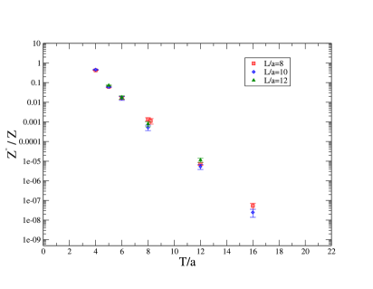
Figure 1: The ratio $Z^{-}/Z$ as a function of $T/a$ for different lattice sizes. The lattice spacing is always $a\simeq 0.17$ fm.

These results demonstrate that the algorithm behaves as expected, and that the multi-level integration scheme indeed achieves an exponential reduction of the numerical effort with respect to the standard procedure. We find quite remarkable that we could follow an exponential decay over almost 7 orders of magnitude and for time separations of about 3 fm. In addition the agreement among the results for different values of $L/a$ shows that at these volumes torelon contributions, if at all present, are negligible.

3 Generalization to the complete set of lattice symmetries

Without fixing a complete set of quantum numbers particle identification is very difficult, even if $T$ is large enough for the partition function restricted to a given sector to be dominated by a single state. For example, in the parity odd sector a superposition of states as

$${{1}\over{\sqrt{2}}}\left(|0^{++},\vec{p}\rangle-|0^{++},-\vec{p}\rangle\right)\;,\quad|\vec{p}|=2\pi/L$$

is contributing and its energy may be smaller than the mass of the lowest parity odd glueball. Such a contribution could of course be removed by projecting on zero spatial momentum. The example shows that for a precision study of the glueball spectrum it is necessary to fix several quantum numbers. The symmetry groups of the lattice SU(3) Yang-Mills theory are

• Charge and Parity conjugation. These are Abelian groups composed by 2 elements each.

• Spatial translations. This is again an Abelian group with $(L/a)^{3}$ elements.

• Central Charge conjugation. This is a symmetry group of the pure gauge theory in a finite volume with periodic boundary conditions [7]. The group is Abelian and is made of 27 elements.

• The Octahedral group of lattice spatial rotations. It is a non-Abelian group composed by 24 transformations.

In general elements from different groups do not commute and therefore only a subset of the associated quantum numbers can be simultaneously fixed. In the following we will show how projectors on irreducible representations of each of the above groups can be introduced in the formalism presented in the previous section [8].

Let us consider one symmetry group of order $g$. The phase space of the theory can be factorized into regular representations constructed by starting from a state $|V\rangle$ and by applying on it all group transformations to obtain the “vectors” $|V^{\Gamma_{i}}\rangle=\hat{\Gamma}_{i}|V\rangle$, $\;i=1\dots g$. Group theory then tells us how to construct the projector $\hat{P}^{(\mu)}$ on the irreducible representation $\mu$ of the group, namely

$$\hat{P}^{(\mu)}={{n_{\mu}}\over{g}}\sum_{i=1}^{g}\chi^{(\mu)*}_{i}\hat{\Gamma}_{i}\;,$$ (5)

where $n_{\mu}$ is the dimension of the irreducible representation, and $\chi^{(\mu)}_{i}$ is the character of the $i$th group element in that representation. The contribution $Z^{(\mu)}$ to the partition function coming from the states transforming in the irreducible representation $\mu$

$$Z^{(\mu)}(T)=\,\hbox{\rm Tr}\left\{\hat{\rm T}^{T}\hat{P}^{(\mu)}\hat{{\rm P}}_{\rm G}\right\}\;,$$ (6)

can be re-written, in fully analogy to what has been done for the case of the partition function restricted to the parity odd states, as (cf eqs. 2-4)

$$Z^{(\mu)}(T)=\int\prod_{i=0}^{T/d-1}{\bf D}_{3}[V_{id}]\left({\rm T}^{(\mu)}\right)^{\!\!d\!}[V_{(i+1)d},V_{id}]\;,$$ (7)

where

$$\left({\rm T}^{(\mu)}\right)^{\!\!d\!}[V_{x_{0}+d},V_{x_{0}}]={{n_{\mu}}\over{g}}\sum_{i=1}^{g}\chi^{(\mu)*}_{i}{\rm T}^{d}[V_{x_{0}+d},V^{\Gamma_{i}}_{x_{0}}]\;,$$ (8)

which extends eq. 4 and reproduces it in the case of the non-singlet representation of the parity group. The basic quantities to be computed in the multilevel algorithm are now the ratios

$${{{\rm T}^{d}\Big{[}V_{x_{0}+d}^{\Gamma_{i}},V_{x_{0}}\Big{]}}\over{{\rm T}^{d}\Big{[}V_{x_{0}+d},V_{x_{0}}\Big{]}}}\;,\quad i=1\dots g\;,$$

and the product over the thick time-slices of proper linear combinations of such quantities is then again integrated over the boundary configurations. When several quantum numbers are fixed the number of ratios to be computed grows as the product of the dimensions of the associated groups. The numerical cost of the algorithm however does not increase accordingly, basically because the accuracy on each single ratio can be relaxed as their number becomes larger [8].

4 Numerical Results

As an explicit example we consider the projector on a given spatial momentum $\vec{p}$. That will be used in most of the cases to project to zero momentum except for the computation of the mass of the lightest $0^{++}$ glueball, where by projecting on a finite momentum we will get rid of the otherwise dominating vacuum contribution. The relative contribution of states with momentum $\vec{p}$ in the system with Dirichlet boundary conditions is given by ($\hat{P}(\vec{x})$ representing translations by $\vec{x}$)

$${{(T^{\vec{p}})^{d}\Big{[}V_{x_{0}+d},V_{x_{0}}\Big{]}}\over{T^{d}\Big{[}V_{x_{0}+d},V_{x_{0}}\Big{]}}}={{1}\over{\sqrt{(L/a)^{3}}}}\sum_{\vec{x}}e^{-i\vec{p}\cdot\vec{x}}{{T^{d}\Big{[}V^{P(\vec{x})}_{x_{0}+d},V_{x_{0}}\Big{]}}\over{T^{d}\Big{[}V_{x_{0}+d},V_{x_{0}}\Big{]}}}\;.$$ (9)

We have implemented the above projection together with the projection on the charge conjugation even sector for some of the $L/a=8$ runs discussed in Section 2. This serves as a test of part of the strategy we plan to follow to eventually compute the mass of the lowest $0^{++}$ glueball state. Results are shown in Fig. 2. We plot the square of an effective energy, defined as $-(\ln(Z^{\vec{p},C=+}/Z))/T$ averaged over the number of momenta $\vec{p}$ with the same $|\vec{p}|^{2}$, versus $|\vec{p}|^{2}$ for different values of $T/a$.

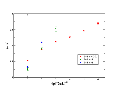
Figure 2: Effective energy from the ratio $Z^{\vec{p},C=+}/Z$ (see text) versus $|\vec{p}|^{2}$ for different $T/a$.

As $T$ becomes large enough for $Z^{\vec{p},C=+}/Z$ to be dominated by a single one-particle state the plot should reproduce a linear dispersion relation and the slope should approach the speed of light value $c^{2}=1$. We see that such a situation is realized for $T/a=6$ and larger values of $T$ produce consistent results tough with larger errors. By extrapolating the $T/a=6$ data to zero momentum we could estimate the mass of the corresponding state with a few percent accuracy. To claim that this state is the $0^{++}$ glueball we however need additional computations in order to exclude parity odd- and higher spin-glueballs [8].

5 Conclusions and outlook

The exponential growth of the noise to signal ratio is one of the main obstructions to precise computations in lattice QCD of observables defined beyond the mesonic sector. In the pure gauge theory this problem can be cured by moving away from importance sampling and the standard approach relying on the computation of two-point functions. We have proposed an algorithm where projectors can be introduced which allow the propagation in time of states with selected quantum numbers only on each gauge configuration. The approach has been tested numerically in the four-dimensional SU(3) Yang-Mills theory by computing the relative contribution of parity odd states to the partition function. In this way we could follow an exponential decay over 7 orders of magnitude and up to time-separations of $3$ fm and verify that the algorithm scales as a power of the time separation for a fixed precision on the rate of the exponential decay.

We are now performing a glueball spectroscopy study in this setup. To this end we have extended the approach to include projectors on all lattice quantum numbers. As a feasibility study of a strategy for the computation of the mass of the lightest $0^{++}$ glueball we have tested the projector on a finite spatial momentum. The results are encouraging, however such a projector is too expensive to be treated exactly and we are currently exploring the efficiency of stochastic implementations [8].

Finally, compared to other approaches, the one we are following offers the possibility to compute in addition the multiplicity of a state, and even more interestingly, to numerically prove the existence of a mass gap in the pure gauge theory [8].

Acknowledgements. The simulations were performed on PC clusters at CERN, at CILEA, at the Swiss National Supercomputing Centre (CSCS) and at the Jülich Supercomputing Centre (JSC). We thankfully acknowledge the computer resources and technical support provided by all these institutions and their technical staff.

References

- [1] G. Parisi, Phys. Rept. 103 (1984) 203.
- [2] G.P. Lepage, TASI 89 Summer School, Boulder, CO, Jun 4-30, 1989.
- [3] M. Della Morte and L. Giusti, Comput. Phys. Commun. 180 (2009) 819.
- [4] M. Lüscher and P. Weisz, JHEP 09 (2001) 010.
- [5] K.G. Wilson, in ”New developments in quantum field theory and statistical mechanics”, Cargèse 1976, Eds. M. Lévy and P. Mitter, Plenum (NY 1977).
- [6] M. Della Morte and L. Giusti, PoS LATTICE2009 (2009) 29, arXiv:0910.2455 [hep-lat].
- [7] G. ’t Hooft, Nucl. Phys. B153 (1979) 141.
- [8] M. Della Morte and L. Giusti, arXiv:1012.2562 [hep-lat].