Hamiltonian Determination with Restricted Access in Transverse Field Ising Chain

Abstract

We propose a method to evaluate parameters in the Hamiltonian of the Ising chain under site-dependent transverse fields, with a proviso that we can control and measure one of the edge spins only. We evaluate the eigenvalues of the Hamiltonian and the time-evoultion operator exactly for a 3-spin chain, from which we obtain the expectation values of $\sigma_{x}$ of the first spin. The parameters are found from the peak positions of the Fourier transform of the expectation value. There are four assumptions in our method, which are mild enough to be satisfied in many physical systems.

1 Introduction

Quantum information processing has been studied for a long time since Feynman’s pioneering work[1, 2, 3]. Many researchers are working toward physical realizations of a practical quantum computer. We have to overcome several obstacles, however, to physically realize a working quantum information processor. One of the main issues is to synthesize a high-quality qubit with a long coherence time. If we prepare a set of high-quality qubits, we have to identify the interaction strengths among qubits with a high degree of accuracy. Without knowing the inter-qubit interactions, it is impossible to control the qubit state at our disposal. In some cases, the majority of the qubits must be isolated from the environment to suppress decoherence, in which case we have an access to a single qubit only. Then we need to find the parameters in the total system, such as the coupling constants, through the single qubit.

There are existing works on evaluation of spin-spin interactions with such a restricted access[4, 5, 6, 7, 8, 9, 10]. Burgarth, Maruyama and Nori[7, 8, 9], studied the Hamiltonian determination in the Heisenberg and the XXZ models with $N$ spins. They took advantage of the fact that the excited states in these systems are classified according to the eigenvalues of a conserved quantity and each excited state belongs to an $N$-dimensional subspace of the total Hilbert space. As a result, it is sufficient to work with this $N$-dimensional subspace in evaluating the parameters in the Hamiltonian.

The purpose of this paper is to extend their analysis to more challenging cases in which the whole $2^{N}$ basis vectors are required to construct an eigenvector. Our particular example studied here is the Ising chain in site-dependent transverse fields. We restrict ourselves mostly within a three-spin chain, the shortest nontrivial chain, to make our analysis concrete. It also turns out that the result is extremely lengthy for a longer spin chain so that it is impossible to write down the results in compact forms.

We introduce our model Hamiltonian and quantum dynamics in the next section. Section 3 is devoted to Hamiltonian determination. Discussion and conclusion are given in Section 4. Details of the calculation are summarized in Appendix.

2 Hamiltonian and Time-Evolution

We investigate, in this paper, how to determine the spin-spin interaction strengths and the external magnetic field strengths in a $3$-spin Ising chain with site-dependent transverse fields. The Hamiltonian is given by

$${\cal H}(h_{i},J_{i})=\sum_{i=1}^{2}J_{i}\sigma_{i}^{z}\sigma_{i+1}^{z}-\sum_{i=1}^{3}h_{i}\sigma_{i}^{x},$$ (1)

where $\sigma_{i}^{x}$ and $\sigma_{i}^{z}$ denote the $x$-component and the $z$-component of the Pauli spin matrices at the $i$-th site, respectively. It is assumed, without loss of generality, that the magnetic field is applied along the $x$-axes of spins 2 and 3 by employing local gauge transformations. This is due to the fact that the dynamics of $\sigma_{1}^{x}$ is independent of the direction of the magnetic fields $h_{2}$ and $h_{3}$ in the $xy$-plane at the sites 2 and 3, respectively. This can be explicitly seen by the identity

$$V^{\dagger}\sigma_{1}^{x}V=\sigma_{1}^{x},$$ (2)

where $V=e^{-i(\alpha_{2}\sigma_{2}^{z}+\alpha_{3}\sigma_{3}^{z})}$ is a transformation which rotates the spins 2 and 3 in the $xy$-plane by angles $\alpha_{2}$ and $\alpha_{3}$, respectively. We take $h_{2}$ and $h_{3}$ to be positive by making use of this freedom from now on.

Our purpose is to evaluate the parameters in the Hamiltonian by controlling and measuring the first spin only. We assume the following four mild conditions to this end:

• It is possible to prepare the fully polarized state $|\uparrow\uparrow\uparrow\rangle$ as an initial state.

• We can control the first spin only. We may prepare the states such as $(\alpha|\uparrow\rangle+\beta|\downarrow\rangle)|\uparrow\uparrow\rangle$ by making use of this assumption.

• Once the initial state is set up, we can control the magnetic field $h_{1}$ at the first site only. Other fields $h_{2}$ and $h_{3}$ are fixed but unknown to us.

• We can measure the spin dynamics of $\sigma_{1}^{x}$ only.

Our proposed scheme is summarized as follows:

Step 1

We prepare an initial state.

Step 2

The dynamics of the $x$-component of the first spin $\langle\sigma_{1}^{x}(t)\rangle$ is measured.

Step 3

The Fourier transform $\hat{\sigma}_{1}^{x}(\omega)$ of $\langle\sigma_{1}^{x}(t)\rangle$ is evaluated.

Step 4

We determine $h_{2},h_{3}$, $|J_{1}|$ and $|J_{2}|$ from the peak positions of $\hat{\sigma}_{1}^{x}(\omega)$ as functions of $h_{1}$.

Step 5

There are four combinations of the signs of $J_{1}$ and $J_{2}$. We evaluate the short time behavior of $\sigma_{1}^{x}(t)$ numerically for each of the four cases and compare the results with that obtained experimentally to determine the signs. (The dynamics is independent of the signs of $h_{2}$ and $h_{3}$ as remarked previously.)

Let $\{\epsilon_{i}\}_{1\leq i\leq 8}$ be the eigenenergies of the Hamiltonian, whose explicit forms in terms of the parameters $\{h_{i},J_{i}\}$ are given by Eq. (31) in Appendix. The eigenenergies of this Hamiltonian satisfy the following symmetry relations:

$$\begin{cases}\epsilon_{5}=-\epsilon_{4}\equiv\epsilon_{\bar{4}}\\ \epsilon_{6}=-\epsilon_{3}\equiv\epsilon_{\bar{3}}\\ \epsilon_{7}=-\epsilon_{2}\equiv\epsilon_{\bar{2}}\\ \epsilon_{8}=-\epsilon_{1}\equiv\epsilon_{\bar{1}}\end{cases}$$ (3)

$$\begin{cases}\epsilon_{1}+\epsilon_{4}=\epsilon_{2}+\epsilon_{3}=-(\epsilon_{\bar{1}}+\epsilon_{\bar{4}})=-(\epsilon_{\bar{2}}+\epsilon_{\bar{3}})\\ \epsilon_{1}-\epsilon_{3}=\epsilon_{2}-\epsilon_{4}=-(\epsilon_{\bar{1}}-\epsilon_{\bar{3}})=-(\epsilon_{\bar{2}}-\epsilon_{\bar{4}})\\ \epsilon_{1}-\epsilon_{2}=\epsilon_{3}-\epsilon_{4}=-(\epsilon_{\bar{1}}-\epsilon_{\bar{2}})=-(\epsilon_{\bar{3}}-\epsilon_{\bar{4}})\end{cases}$$ (4)

Let us choose the fully polarized state $|\uparrow\uparrow\uparrow\rangle$ as an initial state. The state of the chain at time $t>0$ is $|\psi(t)\rangle=U(t)|\uparrow\uparrow\uparrow\rangle$, where $U(t)$ is the time evolution operator

$$U(t) = \exp(-i{\mathcal{H}}t)=\sum_{j=1}^{8}e^{-i\epsilon_{j}t}{\mathcal{P}}_{j}.$$ (5)

Here

$${\mathcal{P}}_{j}=\prod_{\begin{subarray}{c}k=1\\ k\neq j\end{subarray}}^{8}\frac{{\mathcal{H}}-\epsilon_{k}I}{\epsilon_{j}-\epsilon_{k}}$$ (6)

is the projection operator to the eigenspace with the eigenenergy $\epsilon_{j}$. The real-time dynamics $\langle\sigma_{1}^{x}(t)\rangle$ of the first spin is calculated with respect to $|\psi(t)\rangle$ as

$$\left\langle\sigma_{1}^{x}(t)\right\rangle=\langle\psi(t)|\sigma_{1}^{x}|\psi(t)\rangle=C+\sum_{\begin{subarray}{c}m=1\\ m>n\end{subarray}}^{4}\left[A_{mn}\cos\left(\epsilon_{m}+\epsilon_{n}\right)t+B_{mn}\cos\left(\epsilon_{m}-\epsilon_{n}\right)t\right],$$ (7)

where the coefficients $C$, $A_{mn}$ and $B_{mn}$ are functions of $\{J_{i}\}$ and $\{h_{i}\}$. For example, $C$ is explicitly written as

$$C=\langle\uparrow\uparrow\uparrow|\sum_{i=1}^{8}{\mathcal{P}}_{i}\sigma_{1}^{x}{\mathcal{P}}_{i}|\uparrow\uparrow\uparrow\rangle,$$ (8)

while $A_{21}$ and $B_{41}$ are

$$A_{21}=\langle\uparrow\uparrow\uparrow|\left({\mathcal{P}}_{1}\sigma_{1}^{x}{\mathcal{P}}_{7}+{\mathcal{P}}_{2}\sigma_{1}^{x}{\mathcal{P}}_{8}+{\mathcal{P}}_{7}\sigma_{1}^{x}{\mathcal{P}}_{1}+{\mathcal{P}}_{8}\sigma_{1}^{x}{\mathcal{P}}_{2}\right)|\uparrow\uparrow\uparrow\rangle,$$ (9)

and

$$B_{41}=\langle\uparrow\uparrow\uparrow|\left({\mathcal{P}}_{1}\sigma_{1}^{x}{\mathcal{P}}_{4}+{\mathcal{P}}_{4}\sigma_{1}^{x}{\mathcal{P}}_{1}+{\mathcal{P}}_{8}\sigma_{1}^{x}{\mathcal{P}}_{5}+{\mathcal{P}}_{5}\sigma_{1}^{x}{\mathcal{P}}_{8}\right)|\uparrow\uparrow\uparrow\rangle,$$ (10)

respectively.

It is found from Eq. (7) that the peak positions of the Fourier transform $\hat{\sigma}_{1}^{x}(\omega)$ are potentially at $\epsilon_{m}\pm\epsilon_{n}$ for all combinations of $m$ and $n$ ($1\leq m,n\leq 4,m\neq n$). It should be noted, however, that some combinations of $m$ and $n$ have vanishing amplitudes $A_{mn}^{x},B_{mn}^{x}$, for which case the corresponding peaks do not exist. In the present case, it can be shown exactly that

$$A_{41}^{x}=A_{32}^{x}=B^{x}_{21}=B^{x}_{31}=B^{x}_{42}=B^{x}_{43}=0.$$ (11)

These amplitudes satisfy the sum rule

$$C+\sum_{\begin{subarray}{c}m=1\\ m>n\end{subarray}}^{4}(A_{mn}+B_{mn}) = \langle\uparrow\uparrow\uparrow|\left(\sum_{j=1}^{8}{\mathcal{P}}_{j}\right)\sigma_{1}^{x}\left(\sum_{k=1}^{8}{\mathcal{P}}_{k}\right)|\uparrow\uparrow\uparrow\rangle$$ (12)

$$= \langle\uparrow\uparrow\uparrow|\sigma_{1}^{x}|\uparrow\uparrow\uparrow\rangle=0,$$

where use has been made of the completeness relation

$$\sum_{j=1}^{8}{\mathcal{P}}_{j}=I.$$

3 Hamiltonian Determination

Suppose we conducted an experiment and measured $\left\langle\sigma_{1}^{x}(t)\right\rangle$, or equivalently $\hat{\sigma}_{1}^{x}(\omega)$. Now our task is to identify which peak corresponds to which $\epsilon_{m}\pm\epsilon_{n}$ in order to evaluate the parameters $\{J_{i}\}$ and $\{h_{i}\}$. Figure 1 shows $\epsilon_{m}\pm\epsilon_{n}$ with non-vanishing $A_{mn}$ and $B_{mn}$ as functions of the transverse field $h_{1}$, which is assumed to be controllable. Other parameters are arbitrarily chosen as $h_{2}=6$, $h_{3}=7$, $J_{1}=4$ and $J_{2}=5$.

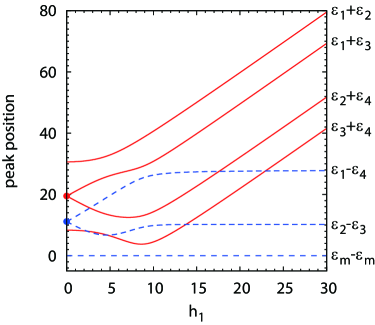
Figure 1: (Color online) Red solid and blue broken curves denote $\epsilon_{m}+\epsilon_{n}$ and $\epsilon_{m}-\epsilon_{n}$, respectively, as functions of the transverse field $h_{1}$ with $h_{2}=6$, $h_{3}=7$, $J_{1}=4$ and $J_{2}=5$. We have plotted the first quadrant part of the graph for simplicity. The peaks in the other quadrants are obtained by mirror reflections of this diagram with respect to the horizontal and/or the vertical axes. The red (blue) dot at $h_{1}=0$ shows the nonvainshing amplitude $A_{\rm II,I}^{0}$ ($B_{\rm II,I}^{0}$).

The red solid curves and blue broken curves in Fig. 1 depict $\epsilon_{m}+\epsilon_{n}$ and $\epsilon_{m}-\epsilon_{n}$, respectively. It should be clear from this diagram that the curves cross intricately for intermediate $h_{1}$, while the behaviors of the curves for small $h_{1}$ and large $h_{1}$ are regular. Then identification of the curves and $\epsilon_{m}\pm\epsilon_{n}$ in these regions is easy. It should be noted here that the case $h_{1}=0$ is singular: $\sigma_{1}^{x}(t)$ remains zero for any $t\geq 0$ for $h_{1}=0$ and $|\psi(0)\rangle=|\uparrow\uparrow\uparrow\rangle$. This case will be treated separately below.

In principle, we may also use the heights (amplitudes) $A_{mn}$ and $B_{mn}$ of theses peaks to determine the parameters. In practice, however, it is rather difficult to use the data for this purpose due to the following reason. First, the analytical expressions for $A_{mn}$ and $B_{mn}$ are extremely lengthy and we need to employ extensive numerical optimization to determine the parameters which fit with the data. Second, the peak has finite width in actual experiment due to various reasons, such as relaxation. We must integrate the peak profile with respect to $\omega$ to find the amplitude, which always suffers from error. In addition, reading off the frequency can be done with much better precision than measuring the amplitude. Figure 2 shows non-vanishing amplitudes as functions of $h_{1}$ for $h_{2}=6$, $h_{3}=7$, $J_{1}=4$ and $J_{2}=5$.

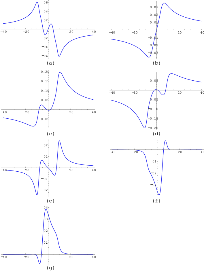
Figure 2: (Color online) Peak amplitudes (a) $C$, (b) $A_{21}$, (c) $A_{31}$, (d) $A_{42}$, (e) $A_{43}$, (f) $B_{41}$ and (g) $B_{32}$ as functions of $h_{1}$. Other parameters are $h_{2}=6$, $h_{3}=7$, $J_{1}=4$ and $J_{2}=5$. All other amplitudes vanish identically.

Peak amplitudes $C$, $A_{21}$ and $A_{43}$ are odd functions of $\omega$ while others are apparently not. Note, however, that the positive-$h_{1}$ (negative-$h_{1}$) part of $A_{31}$ and the negative-$h_{1}$ (positive-$h_{1}$) part of $A_{42}$ combined together define an odd function. The loss of antisymmetry in these amplitudes is due to our choice of the energy eigenvalues (31). If we demand that the eigenvalues be defined uniquely by Eq. (31) for all parameters, we must give up the antisymmetry of the amplitudes $A_{mn}$ and $B_{mn}$. This also happens to the pair $B_{41}$ and $B_{32}$. Figure 2 demonstrates that the sum rule (12) holds for any $h_{1}$.

Let us first consider the limit of a strong magnetic field $h_{1}$, that is, the parameters satisfy $|h_{1}|\gg h_{2},h_{3},|J_{1}|,|J_{2}|$. The non-vanishing Fourier peak positions $\epsilon_{m}+\epsilon_{n}$ $(1\leq m,n\leq 4)$ diverge linearly as $h_{1}\to\infty$. In contrast, the peak positions $\epsilon_{m}-\epsilon_{n}$ converge to constant values. We obtain the asymptotic behavior of $\epsilon_{m}\pm\epsilon_{n}$ for $|h_{1}|\gg h_{2},h_{3},|J_{1}|,|J_{2}|$ from the explicit forms of $\epsilon_{m}$ given in Eq. (31) as

$$\epsilon_{1}+\epsilon_{2}\to 2h_{1}+\left[\sqrt{\left(h_{2}+h_{3}\right)^{2}+J_{2}^{2}}+\sqrt{\left(h_{2}-h_{3}\right)^{2}+J_{2}^{2}}\right]+{\cal O}\left(\frac{1}{h_{1}}\right),$$ (13)

$$\epsilon_{1}+\epsilon_{3}\to 2h_{1}+\left[\sqrt{\left(h_{2}+h_{3}\right)^{2}+J_{2}^{2}}-\sqrt{\left(h_{2}-h_{3}\right)^{2}+J_{2}^{2}}\right]+{\cal O}\left(\frac{1}{h_{1}}\right),$$ (14)

$$\epsilon_{2}+\epsilon_{4}\to 2h_{1}-\left[\sqrt{\left(h_{2}+h_{3}\right)^{2}+J_{2}^{2}}-\sqrt{\left(h_{2}-h_{3}\right)^{2}+J_{2}^{2}}\right]+{\cal O}\left(\frac{1}{h_{1}}\right),$$ (15)

$$\epsilon_{3}+\epsilon_{4}\to 2h_{1}-\left[\sqrt{\left(h_{2}+h_{3}\right)^{2}+J_{2}^{2}}+\sqrt{\left(h_{2}-h_{3}\right)^{2}+J_{2}^{2}}\right]+{\cal O}\left(\frac{1}{h_{1}}\right)$$ (16)

and

$$\epsilon_{1}-\epsilon_{4}\to 2\sqrt{\left(h_{2}+h_{3}\right)^{2}+J_{2}^{2}}+{\cal O}\left(\frac{1}{h_{1}^{2}}\right),$$ (17)

$$\epsilon_{2}-\epsilon_{3}\to 2\sqrt{\left(h_{2}-h_{3}\right)^{2}+J_{2}^{2}}+{\cal O}\left(\frac{1}{h_{1}^{2}}\right).$$ (18)

From these results, we find the ordering of the peak positions for a large $h_{1}$ as

$$\epsilon_{1}+\epsilon_{2}>\epsilon_{1}+\epsilon_{3}>\epsilon_{2}+\epsilon_{4}>\epsilon_{3}+\epsilon_{4}$$ (19)

and

$$\epsilon_{1}-\epsilon_{4}>\epsilon_{2}-\epsilon_{3}.$$ (20)

Once the peak positions are identified with particular $\epsilon_{m}\pm\epsilon_{n}$, we may easily find $\sqrt{\left(h_{2}+h_{3}\right)^{2}+J_{2}^{2}}$ and $\sqrt{\left(h_{2}-h_{3}\right)^{2}+J_{2}^{2}}$ numerically. Clearly these two numbers are not sufficient to determine the four parameters in the Hamiltonian and we need to examine the peaks at other values of $h_{1}$, such as $h_{1}=0$, to acquire sufficient data to completely determine the parameters.

We note en passant that the asymptotic behavior of the peaks does depend on $J_{2}$ but not on $J_{1}$. This counter-intuitive character is understood if we study the perturbation theory at $h_{1}\to\infty$. Let us separate the Hamiltonian as

$${\cal H}={\cal H}_{0}+{\cal H}_{\rm 1},$$ (21)

$${\cal H}_{0}=-h_{1}\sigma_{1}^{x},$$ (22)

$${\cal H}_{\rm 1}=\sum_{i=1}^{2}J_{i}\sigma_{i}^{z}\sigma_{i+1}^{z}-\sum_{i=2}^{3}h_{i}\sigma_{i}^{x}.$$ (23)

The eigenvectors of the unperturbed Hamiltonian ${\cal H}_{0}$ are $\frac{1}{\sqrt{2}}(|\!\uparrow\rangle\pm|\!\downarrow\rangle)|s_{2}s_{3}\rangle$, where $s_{2},s_{3}\in\{\uparrow,\downarrow\}$. The first order perturbation of the eigenvalues is independent of $J_{1}$, which is why the asymptotic eigenenergies are independent of $J_{1}$. This behavior is also understood from the spin dynamics. When the magnetic field $h_{1}$ is much larger than the other parameters, the characteristic time $\tau$ of the motion of the first spin is very short compared to other characteristic times. Then the effect of the spin-spin interaction $J_{1}$ is averaged to vanish over the time interval $t\gg\tau$ and the $J_{1}$ interaction is ignored in this limit. Clearly this remains true for any number of spins in the chain.

Next we consider the case when $h_{1}=0$ to acquire sufficient data to fix all the parameters. The eigenenergies in this case are $\pm\epsilon_{\rm I},\pm\epsilon_{\rm II}$, each of which is doubly degenerate. Here we take $\epsilon_{\rm I}>\epsilon_{\rm II}>0$. The explicit forms of $\epsilon_{\rm I,II}$ are given by Eq. (48) in Appendix. It is easy to show that

$$\langle\uparrow\uparrow\uparrow|U(t)^{\dagger}\sigma_{1}^{x}U(t)|\uparrow\uparrow\uparrow\rangle=0$$

for $h_{1}=0$. This is an artifact of the initial state chosen above. Note that $\sigma_{1}^{x}$ does not commute with the Hamiltonian and a proper initial condition introduces a nontrivial expectation value of the observable. Let us take an initial state $|+\uparrow\uparrow\rangle$, where

$$|+\rangle=\frac{1}{\sqrt{2}}(|\!\uparrow\rangle+|\!\downarrow\rangle).$$

Then the real-time dynamics $\langle\sigma_{1}^{x}(t)\rangle$ is calculated as

$$\left\langle\sigma_{1}^{x}(t)\right\rangle=C+A_{\rm II,I}^{0}\cos\left(\epsilon_{\rm I}+\epsilon_{\rm II}\right)t+B_{\rm II,I}^{0}\cos\left(\epsilon_{\rm I}-\epsilon_{\rm II}\right)t,$$ (24)

where the coefficients $C$, $A_{\rm II,I}^{0}$ and $B_{\rm II,I}^{0}$ are functions of $\{J_{i}\}$ and $\{h_{i}\}$, whose explicit forms are given in Eq. (53).

The peak positions with nonvanishing amplitudes at $h_{1}=0$ are

$$\omega=\epsilon_{\rm I}\pm\epsilon_{\rm II}=\sqrt{S_{0}+2\sqrt{C_{0}}}\pm\sqrt{S_{0}-2\sqrt{C_{0}}},$$ (25)

and $\omega=0$, where

$$S_{0}=h_{2}^{2}+h_{3}^{2}+J_{1}^{2}+J_{2}^{2},\ C_{0}=h_{2}^{2}h_{3}^{2}+h_{3}^{2}J_{1}^{2}+J_{1}^{2}J_{2}^{2}.$$ (26)

Since peak positions $\epsilon_{\rm I}\pm\epsilon_{\rm II}$ produce only two numbers $\sqrt{S_{0}\pm 2\sqrt{C_{0}}}$, which are essentially the same as $S_{0}$ and $C_{0}$, we should combine the data acquired for the case of a large $h_{1}$ to determine all the parameters $h_{2}$, $h_{3}$, $|J_{1}|$ and $|J_{2}|$. Once all the non-vanishing peak positions are identified, the measurement of the peaks of $\hat{\sigma}_{1}^{x}(\omega)$ for additional finite $h_{1}$ helps us determine the parameters with higher precision. Figure 2 shows that all the peak amplitudes decay as $h_{1}\to\infty$. It may happen that the peaks are not observable at large enough $h_{1}$ since their amplitudes vanish in this region. If this is the case, we need to identify peaks at $h_{1}=0$ first and then sweep $h_{1}$ to acquire sufficient data to determine the parameters.

For the parameter choice, $h_{1}=0,h_{2}=6,h_{3}=7,J_{1}=4$ and $J_{2}=5$, we obtain the amplitudes numerically as

$$C=0.5984,\ A_{\rm II,I}^{0}=0.05525,\ B_{\rm II,I}^{0}=0.3464.$$ (27)

They do not agree with the $h_{1}\to 0$ limit in Fig. 2 since their initial states are different. These amplitudes satisfy a sum rule different from Eq. (12),

$$C+A_{\rm II,I}^{0}+B_{\rm II,I}^{0}=\langle+\uparrow\uparrow|\sigma_{1}^{x}|+\uparrow\uparrow\rangle=1.$$ (28)

Now that $h_{2}$, $h_{3}$, $|J_{1}|$ and $|J_{2}|$ are determined, our next task is to find the signs of $J_{1}$ and $J_{2}$. Figure 3 shows the dynamics of $\sigma_{1}^{x}$ for $|J_{1}|=4$, $|J_{2}|=5$, $h_{1}=1$, $h_{2}=6$, and $h_{3}=7$ for the four combinations of the signs of $J_{1}$ and $J_{2}$. The signs are $({\rm sign}(J_{1}),{\rm sign}(J_{2}))=(+,+)$, $(-,+)$, $(+,-)$, and $(-,-)$ from top to bottom. We immediately note that $\sigma_{1}^{x}(t)$ is positive (negative) for small time limit if ${\rm sign}(J_{1})$ is negative (positive). This is because the molecular field at the first site is approximately $(-h_{1},0,J_{1})$ for small $t$. Thus sign($J_{1}$) is fixed by inspecting the short time dynamics of $\langle\sigma_{1}^{x}(t)\rangle$. Unfortunately, sign($J_{2}$) cannot be determined in this way. We also note that the dynamics $\langle\sigma_{1}^{x}(t)\rangle$ changes the sign under the transformation $(J_{1},J_{2})\to(-J_{1},-J_{2})$ as seen from Fig. 3. This is due to the following identities,

$$X_{2,\pi}(-\sum_{i=1}^{3}h_{i}\sigma_{i}^{x}+\sum_{i=1}^{2}J_{i}\sigma_{i}^{z}\sigma_{i+1}^{z})X_{2,\pi}^{\dagger}=-\sum_{i=1}^{3}h_{i}\sigma_{i}^{x}-\sum_{i=1}^{2}J_{i}\sigma_{i}^{z}\sigma_{i+1}^{z}$$ (29)

and

$$\langle\uparrow\uparrow\uparrow|e^{i{\mathcal{H}}(h_{i},-J_{i})t}\sigma_{1}^{x}e^{-i{\mathcal{H}}(h_{i},-J_{i})t}|\uparrow\uparrow\uparrow\rangle$$ (30)

$$= \langle\uparrow\uparrow\uparrow|X_{2,\pi}^{\dagger}e^{i{\mathcal{H}}(h_{i},J_{i})t}X_{2,\pi}\sigma_{1}^{x}X_{2,\pi}^{\dagger}e^{-i{\mathcal{H}}(h_{i},J_{i})t}X_{2,\pi}|\uparrow\uparrow\uparrow\rangle$$

$$= -\langle\uparrow\uparrow\uparrow|e^{i{\mathcal{H}}(h_{i},J_{i})t}\sigma_{1}^{x}e^{-i{\mathcal{H}}(h_{i},J_{i})t}|\uparrow\uparrow\uparrow\rangle,$$

where $X_{2,\pi}=\exp(-i\sigma_{2}^{x}\pi/2)$ is a unitary matrix corresponding to a rotation of the spin 2 around the $x$-axis by an angle $\pi$.

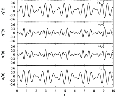
Figure 3: Dynamics of $\sigma_{1}^{x}(t)$ for $({\rm sign}(J_{1}),{\rm sign}(J_{2}))=(+,+)$, $(-,+)$, $(+,-)$, and $(-,-)$, where the Hamiltonian parameters are $h_{1}=1$, $h_{2}=6$, $h_{3}=7$, $|J_{1}|=4$ and $|J_{2}|=5$.

4 Summary and Discussion

In this paper, we propose a method to evaluate the spin-spin interaction strengths and the site-dependent magnetic field strengths only through one of the edge spins. We consider a three-spin Ising model with site-dependent transverse fields $h_{i}$. Since the Ising model with transverse fields has no good quantum number such as the total $S^{z}$, which the Heisenberg and the XXZ models have, it is considerably more difficult to evaluate the parameters in the Hamiltonian in this case.

First a fully polarized state $|\uparrow\uparrow\uparrow\rangle$ (when $h_{1}\neq 0$) or $\frac{1}{\sqrt{2}}(|\uparrow\rangle+|\downarrow\rangle)|\uparrow\uparrow\rangle$ (when $h_{1}=0$) is prepared and the time-dependence of the $x$-component of the first spin is measured. The peak positions of the Fourier transform $\hat{\sigma}_{1}^{x}(\omega)$ are at $\{\epsilon_{m}\pm\epsilon_{n}\}$, where $\epsilon_{n}$ is the first four eigenvalues of the Hamiltonian. The identification of each peak position with a particular $\epsilon_{m}\pm\epsilon_{n}$ is easy for $h_{1}=0$ and $h_{1}\to\infty$, while it is difficult for a finite $h_{1}$ in general. Of course, it is possible to identify the peaks for a finite $h_{1}$ if $h_{1}$ is swept from $0$ to a large value continuously.

We determine $\{h_{i}\}$ and $\{|J_{i}|\}$ completely from the peak positions of $\sigma_{1}^{x}(\omega)$. It was shown that some possible peaks are not observable since they have vanishing amplitudes. Some combinations of the parameters are read off from the peak positions at large $h_{1}$ and $h_{1}=0$. The combined data is sufficient to fix all the parameters completely. Additional data obtained for finite $h_{1}$ improves accuracy of the estimated parameters. The signs of the spin-spin interactions are found by comparing the experimentally obtained spin dynamics with numerical simulation.

In our proposed method, there are only four mild conditions which are satisfied in many experimental systems such as a liquid state NMR quantum computer, which is abbreviated as “an NMR quantum computer” hereafter. In fact, the Ising model with site-dependent transverse field is a typical system in an NMR quantum computer. It is possible to control the magnetic field strength $h_{i}$ of each spin independently by making coordinate transformation to a rotating frame of each spin rotating with the respective Lamour frequency, It should be noted, however, that there is a subtle problem in an NMR quantum computer associated with the initial state. The initial pure state is prepared as a pseudo-pure state, which is produced by the time-average or the space-average method, for example.[12, 13, 14, 15, 16] To produce a pseudo-pure state, however, we need to know the Hamiltonian in advance, which is “the chicken or the egg” causality dilemma. The best we can do is to prepare a pseudo-pure state with a molecule with a known Hamiltonian and then pretend as if we do not know the Hamiltonian and demonstrate our method. We believe our scheme can be experimentally demonstrated also with other physical systems with a pure state.

The authors are grateful to Daniel Burgarth and Koji Maruyama for valuable comments and discussions. This work is partially supported by ‘Open Research Center’ Project for Private Universities: matching fund subsidy from MEXT, Japan. The authors thank the Yukawa Institute for Theoretical Physics at Kyoto University. Discussions during the YITP workshop YITP-W-10-14 on “Duality and Scale in Quantum-Theoretical Sciences” were useful to complete this work. S.T. is partly supported by Grant-in-Aid for Young Scientists Start-up (21840021) from the JSPS and by MEXT Grant-in-Aid for Scientific Research (B) (22340111). The computation in the present work was performed on computers at the Supercomputer Center, Institute for Solid State Physics, University of Tokyo.

Appendix A Derivation of Physical Quantities

A.1 Eigenenergies

After straightforward but tedious calculation, eigenenergies of the Hamiltonian (1) are obtained explicitly as:

$$\begin{cases}\displaystyle\epsilon_{1}=\frac{\alpha}{2}+\frac{\left(\beta+\gamma\right)^{1/2}}{2}\\ \displaystyle\epsilon_{2}=\frac{\alpha}{2}+\frac{\left(\beta-\gamma\right)^{1/2}}{2}\\ \displaystyle\epsilon_{3}=\frac{\alpha}{2}-\frac{\left(\beta-\gamma\right)^{1/2}}{2}\\ \displaystyle\epsilon_{4}=\frac{\alpha}{2}-\frac{\left(\beta+\gamma\right)^{1/2}}{2}\\ \end{cases}\hskip 28.45274pt\begin{cases}\epsilon_{5}=-\epsilon_{4}\equiv\epsilon_{\bar{4}}\\ \epsilon_{6}=-\epsilon_{3}\equiv\epsilon_{\bar{3}}\\ \epsilon_{7}=-\epsilon_{2}\equiv\epsilon_{\bar{2}}\\ \epsilon_{8}=-\epsilon_{1}\equiv\epsilon_{\bar{1}}\\ \end{cases}$$ (31)

where

$$\alpha=\sqrt{\frac{1}{3}\left(4S+\frac{B}{A}+\frac{A}{2^{1/3}}\right)},\ \beta=\frac{1}{3}\left(8S-\frac{B}{A}-\frac{A}{2^{1/3}}\right),\ \gamma=\frac{16h_{1}h_{2}h_{3}}{\alpha},$$

$$S=h_{1}^{2}+h_{2}^{2}+h_{3}^{2}+J_{1}^{2}+J_{2}^{2},\ A=\left[X+\sqrt{-256\left(S^{2}+3\sqrt{{\rm det}{\cal H}}\right)^{3}+X^{2}}\right]^{1/3},$$

$$X=16\left[-S^{3}+9S\sqrt{{\rm det}{\cal H}}+108h_{1}^{2}h_{2}^{2}h_{3}^{2}\right],\ B=2^{7/3}\left[S^{2}+3\sqrt{{\rm det}{\cal H}}\right],$$ (32)

$$\sqrt{{\rm det}{\cal H}}=h_{1}^{4}+h_{2}^{4}+\left(h_{3}^{2}-J_{1}^{2}+J_{2}^{2}\right)^{2}$$

$$\qquad\qquad-2h_{1}^{2}\left(h_{2}^{2}+h_{3}^{2}-J_{1}^{2}+J_{2}^{2}\right)+2h_{2}^{2}\left(-h_{3}^{2}+J_{1}^{2}+J_{2}^{2}\right).$$

Figure 4 shows the eigenenergies as functions of the transverse field $h_{1}$ with $J_{1}=4$, $J_{2}=5$, $h_{2}=6$, and $h_{3}=7$. All eigeneneries are doubly degenerate when $h_{1}=0$.

The eigenenergies $\epsilon_{4}$ and $\epsilon_{5}$ cross when $\epsilon_{4}=\epsilon_{5}=0$, which seems to be in contradiction with the no-level crossing theorem [17]. Nonetheless this is allowed since the eigenvectors corresponding to these degenerate eigenenergies are symmetric and antisymmetric states with respect to the spin indices. The symmetric state and antisymmetric states are characterized by introducing the parity operator [18]:

$${\cal X}=\sigma_{1}^{x}\otimes\sigma_{2}^{x}\otimes\sigma_{3}^{x}.$$ (33)

The Hamiltonian and the parity operator commute:

$$[{\cal H},{\cal X}]=0.$$ (34)

Symmetric and antisymmetric functions are defined as follows:

$$|\Psi_{\rm s}\rangle={\sum_{\left\{s\right\}}}^{\prime}a_{s}\left(|s\rangle+{\cal X}|s\rangle\right),$$ (35)

$$|\Psi_{\rm as}\rangle={\sum_{\left\{s\right\}}}^{\prime}a_{s}\left(|s\rangle-{\cal X}|s\rangle\right),$$ (36)

where $|s\rangle=|s_{1}s_{2}s_{3}\rangle$ denotes a spin configuration, and $\sum_{\left\{s\right\}}^{\prime}$ denotes summation over all spin configurations with $s_{1}=+1$. Observe that ${\cal X}|\Psi_{\rm s}\rangle=|\Psi_{\rm s}\rangle$ while ${\cal X}|\Psi_{\rm as}\rangle=-|\Psi_{\rm as}\rangle$. The eigenstates with the eigenenergies $\epsilon_{4}$ and $\epsilon_{5}$ belong to different symmetry classes and their eigenenergies may cross as $h_{1}$ is changed.

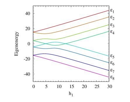
Figure 4: (Color online) Eigenenergies as functions of $h_{1}$ when $J_{1}=4$, $J_{2}=5$, $h_{2}=6$, and $h_{3}=7$.

A.2 $h_{1}=0$ Case

It was shown in the main text that the measurement of the peak positions of $\hat{\sigma}_{1}^{x}(\omega)$ at a large $h_{1}$ was not sufficient to determine the parameters in the Hamiltonian. Let us look at the spin dynamics at $h_{1}=0$ to obtain information required to determine the parameters. The initial condition $|\uparrow\uparrow\uparrow\rangle$ leads $\langle\sigma_{1}^{x}(t)\rangle=0$ for any $t$. Let us take the initial state $\frac{1}{\sqrt{2}}(|\uparrow\rangle+|\downarrow\rangle)|\uparrow\uparrow\rangle$l, instead, to avoid this problem.

The Hamiltonian is block-diagonalized when $h_{1}=0$ as

$${\cal H}=\left(\begin{array}[]{cc}{\cal H}_{u}&0\\ 0&{\cal H}_{d}\end{array}\right),$$ (37)

where

$${\cal H}_{u} = \left(\begin{array}[]{cccc}J_{1}+J_{2}&-h_{3}&-h_{2}&0\\ -h_{3}&J_{1}-J_{2}&0&-h_{2}\\ -h_{2}&0&-J_{1}-J_{2}&-h_{3}\\ 0&-h_{2}&-h_{3}&-J_{1}+J_{2}\end{array}\right),$$ (42)

$${\cal H}_{d} = \left(\begin{array}[]{cccc}-J_{1}+J_{2}&-h_{3}&-h_{2}&0\\ -h_{3}&-J_{1}-J_{2}&0&-h_{2}\\ -h_{2}&0&J_{1}-J_{2}&-h_{3}\\ 0&-h_{2}&-h_{3}&J_{1}+J_{2}\end{array}\right).$$ (47)

The Hamiltonian has four eigenvalues $\pm\epsilon_{\rm I},\pm\epsilon_{\rm II}$, each of which is doubly degenerate. Here

$$\epsilon_{\rm I}=\sqrt{S_{0}+2\sqrt{C_{0}}},\\ \ \epsilon_{\rm II}=\sqrt{S_{0}-2\sqrt{C_{0}}}$$ (48)

with

$$S_{0}=h_{2}^{2}+h_{3}^{2}+J_{1}^{2}+J_{2}^{2},\ C_{0}=h_{2}^{2}h_{3}^{2}+h_{3}^{2}J_{1}^{2}+J_{1}^{2}J_{2}^{2}.$$ (49)

By using projection operators, time-evolution operators are expressed as

$$U_{u} = {\rm e}^{-i{\cal H}_{u}t}=\sum_{k=1}^{4}{\cal P}^{(u)}_{k}{\rm e}^{-i\epsilon_{k}t}$$ (50)

$$= \sum_{\alpha\in\{\rm I,II\}}\left[{\cal P}^{(u)}_{\alpha}{\rm e}^{-i\epsilon_{\alpha}t}+{\cal P}^{(u)}_{\bar{\alpha}}{\rm e}^{-i\epsilon_{\bar{\alpha}}t}\right]$$

$$= \sum_{\alpha\in\{\rm I,II\}}\left[{\cal Q}_{\alpha}^{(u)}\cos(\epsilon_{a}t)+{\cal R}_{\alpha}^{(u)}\sin(\epsilon_{\alpha}t)\right],$$

$$U_{d} = {\rm e}^{-i{\cal H}_{d}t}=\sum_{k=1}^{4}{\cal P}^{(d)}_{k}{\rm e}^{-i\epsilon_{k}t}$$ (51)

$$= \sum_{\alpha\in\{\rm I,II\}}\left[{\cal P}^{(d)}_{\alpha}{\rm e}^{-i\epsilon_{\alpha}t}+{\cal P}^{(d)}_{\bar{\alpha}}{\rm e}^{-i\epsilon_{\bar{\alpha}}t}\right]$$

$$= \sum_{\alpha\in\{\rm I,II\}}\left[{\cal Q}_{\alpha}^{(d)}\cos(\epsilon_{a}t)+{\cal R}_{\alpha}^{(d)}\sin(\epsilon_{\alpha}t)\right],$$

where

$${\cal Q}_{\alpha}^{(u,d)}={\cal P}_{\alpha}^{(u,d)}+{\cal P}_{\bar{\alpha}}^{(u,d)},{\cal R}_{\alpha}^{(u,d)}={i}\left[{\cal P}_{\alpha}^{(u,d)}+{\cal P}_{\bar{\alpha}}^{(u,d)}\right].$$ (52)

Then, real-time dynamics of $x$-component of the first spin is obtained as

$$\langle\sigma_{1}^{x}(t)\rangle = \frac{h_{2}^{2}h_{3}^{2}}{C_{0}}+A_{\rm II,I}^{0}\cos[(\epsilon_{\rm I}+\epsilon_{\rm II})t]+B_{\rm II,I}^{0}\cos[(\epsilon_{\rm I}-\epsilon_{\rm II})t],$$ (53)

where

$$\begin{array}[]{c}\displaystyle A_{\rm II,I}^{0}=\frac{J_{1}^{2}[h_{2}^{2}(h_{3}^{2}-J_{2}^{2})-(h_{3}^{2}+J_{2}^{2})(h_{3}^{2}-J_{1}^{2}+J_{2}^{2})+(J_{2}^{2}+h_{3}^{2})\epsilon_{\rm I}\epsilon_{\rm II}]}{2\epsilon_{\rm I}\epsilon_{\rm II}C_{0}},\vspace{.3cm}\\ \displaystyle B_{\rm II,I}^{0}=\frac{J_{1}^{2}[h_{2}^{2}(-h_{3}^{2}+J_{2}^{2})+(h_{3}^{2}+J_{2}^{2})(h_{3}^{2}-J_{1}^{2}+J_{2}^{2})+(J_{2}^{2}+h_{3}^{2})\epsilon_{\rm I}\epsilon_{\rm II}]}{2\epsilon_{\rm I}\epsilon_{\rm II}C_{0}}.\end{array}$$ (54)

References

- [1] P.W. Shor: in Proceedings of the 35th Annual Symposium on Foundations of Computer Science (IEEE Press, Los Almaitos, 1994) 124.
- [2] M.A. Nielsen and I.L. Chuang: Quantum Computation and Quantum Information (Cambridge University Press, Cambridge, 2000).
- [3] M. Nakahara and T. Ohmi: Quantum Computing From Linear Algebra to Physical Realizations, (CRC Press, Boca Raton, 2008).
- [4] M. Mohseni and D.A. Lider, Phys. Rev. Lett. 97 170501 (2006).
- [5] R. Blume-Kohout, H.K. Ng, D. Poulin, and L. Viola, Phys. Rev. Lett. 100 030501 (2008).
- [6] A. Bendersky, F. Pastawski, and J.P. Paz, Phys. Rev. Lett. 100 190403 (2008).
- [7] D. Burgarth, K. Maruyama, and F. Nori, Phys. Rev. A 79 020305 (2009).
- [8] D. Burgarth and K. Maruyama, New. J. Phys. 11 103019 (2009).
- [9] D. Burgarth, K. Maruyama, and F. Nori, arXiv:1004.5018.
- [10] Y. Shikano and S. Tanaka, arXiv:1007.5370.
- [11] Y. Kondo, J. Phys. Soc. Jpn. 76 104004 (2007).
- [12] E. Knill, I. L. Chuang and R. Laflamme, Phys. Rev. A 81, 5672 (1998).
- [13] D. G. Cory, A. F. Fahmy and T. F. Havel, Proc. Natl. Acad. Sci. USA 94, 1634 (1997).
- [14] U. Sakaguchi, H. Ozawa and T. Fukumi, Phys. Rev. A 61, 042313 (2000).
- [15] N. A. Gershenfeld and I. L. Chuang, Science 275, 350 (1997).
- [16] L. M. K. Vandersypen et al., Phys. Rev. Lett. 83, 3085 (1999).
- [17] P. D. Lax: Linear Algebra and Its Applications, (Wiley-Interscience, Hoboken, New Jersey, 2007).
- [18] S. Tanaka, M. Hirano, and S. Miyashita, Phys. Rev. E 81 051138 (2010).