Abstract

A numerical study of the Faddeev equation for bosons is made with two-body interactions at or close to the Unitary limit. Separable interactions are obtained from phase-shifts defined by scattering length and effective range. In EFT-language this would correspond to NLO. Both ground and Efimov state energies are calculated. For effective ranges $r_{0}>0$ and rank-1 potentials the total energy $E_{T}$ is found to converge with momentum cut-off $\Lambda$ for $\Lambda>\sim 10/r_{0}$ . In the Unitary limit ($1/a=r_{0}=0$) the energy does however diverge. It is shown (analytically) that in this case $E_{T}=E_{u}\Lambda^{2}$. Calculations give $E_{u}=-0.108$ for the ground state and $E_{u}=-1.\times 10^{-4}$ for the single Efimov state found. The cut-off divergence is remedied by modifying the off-shell t-matrix by replacing the rank-1 by a rank-2 phase-shift equivalent potential. This is somewhat similar to the counterterm method suggested by Bedaque et al. This investigation is exploratory and does not refer to any specific physical system.

1 Introduction

Systems involving particles with 2-body interactions at or close to the Unitary limit have become of specific interest in the physics community during the last several years for reasons that have repeatedly been pointed out in numerous publications related to both atomic and sub-atomic problems. The Unitary limit is here defined as being that for which the scattering length $a$ and effective range $r_{0}$ are infinite and zero respectively. In that case the only scale left in a system of fermions of ’infinite’ extension would be the Fermi-momentum. The total energy would then have to be proportional to the Fermi-energy as that is the only scale left in this problem. Experimental results point to $E_{T}\sim 0.44E_{F}$ with $E_{F}$ being the kinetic energy of the ’unperturbed’ kinetic energy of the system. Theoretical determination of the this universal constant is a many-body problem. It should however only involve some simple constants and might aṕriori seem straightforward. It has however been found to be a theoretical challenge. Some calculations of the author using Brueckner methods show for example a very strong dependence on the effective range $r_{0}$. There is also in any theoretial calculation a necessary cut-off $\Lambda$ in momentum-space that renders the 2-body interaction a function of this $\Lambda$. This does introduce another length parameter into the theory. In the previous work of the author, and shown below, the rank-1 separable interaction is in the Unitary limit singular at the momentum $\Lambda$. This fact introduces another problem; the applicability of a many-body theory in this limit. The applicability of the Bruckner method was for example questioned after the realisation of the very large correlations and consequently, ”wound-integral” in this case. The ”model” space represented by a zero-temperature Fermi distribution is no longer adequate. A Green’s function method including spectral broadening would be more appropriate.

As opposed to the ’infinite’ system the three-body system is exactly solvable by the Faddeev method [1]. It therefore presents a more interesting project for a numerical study with interactions at and near the Unitary limit. Of specific interest here is also the phenomena first brought to the attention by Vitali Efimov. [2, 3] He found the surprising fact that bosons interacting with a resonance in the 2-body state (i.e. $1/a\sim 0$) would result in a strongly bound three-body system and with a spectrum of loosely bound excited states.

The inverse scattering method as applied here uses two-body on-shell data (scattering length and effective range) as input. Although on-shell properties of the t-matrix are fitted exactly, many-body calculations involve also off-shell t-matrix elements. These are not derivable from experimental two-body data. So even if a rank-1 potential is sufficient to fit the on-shell data as is often the case it leaves the off-shell undetermined. The extension to a rank-2 will allow for a phase-shift equivalent interaction with different off-shell t-matrix elements. This provides a practical tool for exploring off-shell or equivalently, three-body effects. This method will be used in some cases below. It was used by the author in earlier work. (see e.g. [11]) The on-shell data relate to the asymptotic form of the two-body scattering wave-function. These have to be preserved when increasing the rank which implies that the interaction should be modified at short range in coordinate space as shown below.

In the present report we focus only on the ground and Efimov state energies, as well as on the dependence on scattering lengths and effective ranges and on the questions of convergence as a function of cut-off in momentum-space.

In Section 2 is found a presentation of the necessary tools which are the Faddeev equation and the inverse scattering method. Section 3 show results of numerical calculations in 3 subsections wth 8 Figures. Section 4 is a summary and some discussion of the results.

2 Formalism

The Faddeev three-boson equation for a spin-independent rank-1 separable attractive potential $V(k,k^{\prime})=-v(k)v(k^{\prime})$ is given by

$$\chi(q)=\frac{2}{{\cal I}(E_{T}-\frac{3}{4}q^{2})}\int_{0}^{\Lambda}\frac{v(|{\bf k}+\frac{1}{2}{\bf q}|)v(|{\bf q}+\frac{1}{2}{\bf k}|)}{q^{2}+{\bf q}\cdot{\bf k}+k^{2}-E_{T}}\chi(q)d{\bf k}$$ (1)

with

$${\cal I}(s)=1+\frac{1}{2\pi^{2}}\int_{0}^{\Lambda}v^{2}(k)(s-k^{2})^{-1}k^{2}dk$$ (2)

The extension to the rank-2 potentials used below in Section 3.2 is straight-forward. [4, 5]

The separable interactions are calculated from phase-shifts by an inverse scattering method that dates back at least some 40 years. [6] Some recent applications by the author can be found in refs where details can be found.[7, 8, 9, 14, 10, 11] where some details of the method are also shown. The input are phase-shifts which in general can be either experimental or otherwise defined. For the purpose of this investigation they will be defined by a scattering length $a$ and and an effective range $r_{0}$. A rank-1 separable potential is then sufficient to reproduce the input phase-shifts exactly. (If the phase-shift were to changes sign such as in the nuclear ${}^{1}S_{0}$ case a rank two potential is necessary. [7]). As mentioned above a higher rank may be required in order to accomodate three-body data. The present work is not specific to any particular system other than that the 2-body interaction is close to the Unitary limit for which universality would apply. It is shown however that an off-shell correction (three-body force) via a rank-2 potential can be used to prevent the ultraviolet divergence and collapse of the three-boson system in that limit.

In the case of a rank-1 attractive potential one has

$$V(k,k^{\prime})=-v(k)v(k^{\prime})$$ (3)

Inverse scattering then yields (e.g. ref [7, 6])

$$v^{2}(k)=\frac{(4\pi)^{2}}{k}sin\delta(k)|D(k^{2})|$$ (4)

where

$$D(k^{2})=\frac{k^{2}+E_{B}}{k^{2}}exp\left[\frac{2}{\pi}{\cal P}\int_{0}^{\Lambda}\frac{k^{\prime}\delta(k^{\prime})}{k^{2}-k^{\prime 2}}dk^{\prime}\right]$$ (5)

where ${\cal P}$ denotes the principal value and $\delta(k)$ are the phaseshifts. $\Lambda$ provides a cut-off in momentum-space and the interaction is fully defined by the phase-shifts,the two-body binding energy $E_{B}$ and by $\Lambda$. The effect of the cut-off will be exploited below. $E_{B}$ is calculated from

$$\sqrt{(}E_{B})=\frac{1}{a}+\frac{1}{2}r_{0}E_{B}$$ (6)

It is set to zero for unbound states.

For the rank-2 potentials that are used in Sect. 3.2 the method of Chadan and Fiedeldey was applied.[12, 13] (see also ref. [7]). In this a set of initial phaseshifts is assumed to be provided. An arbitrary interaction $V_{1}$, is then assumed, defined either by another set of phases or explicitly. A second potential, $V_{2}$ can then be constructed so that the rank-2 potential given by $V_{1}$ and $V_{2}$ reproduce the initial phases. If the initial phases are, as in our case below, all of the same sign, they can be reproduced by a rank-1 potential from eq. (4). The extension to a rank-2 potential, allows for an arbitrary change of off-shell behaviour or in other words of the three-body term while preserving the fit to the initial two-body phase-shifts.

With $\delta(k)=\frac{\pi}{2}$, the unitary limit, these phases can be reproduced by a rank one-potential and one finds (e.g.[11])

$$v_{u}^{2}(k)=-\lambda\frac{(4\pi)^{2}}{(\Lambda^{2}-k^{2})^{\frac{1}{2}}}$$ (7)

where the factor $\lambda$ ($=1$ in the unitary limit) is introduced for later presentation of results where the three-boson binding is calculated as a function of this strength factor. Note that $v_{u}^{2}(k)$ $\rightarrow-\infty$ for $k\rightarrow\Lambda$.

Note also that for $\Lambda\gg k$ one finds

$$v_{u}^{2}(k)\rightarrow-\lambda\frac{(4\pi)^{2}}{\Lambda}$$ (8)

In this limit, but only in this limit , the unitary interaction will then be a $\delta$-function in coordinate space with the strength inversely proportional to the cut-off. But eq. (7) shows that a finite $\Lambda$ results in an abrupt increase in strength and a singularity at $k=\Lambda$ to preserve the condition $\delta=\frac{\pi}{2}$ for all $k\leq\Lambda$.

With the interaction (7) and with the momenta in units of the cut-off $\Lambda$ ($k_{\Lambda}=k/\Lambda$ and $q_{\Lambda}=q/\Lambda$) the Faddeev equation is:

$$\chi(q)=\frac{2\lambda}{{\cal I}(E_{u}(\lambda)-\frac{3}{4}q_{\Lambda}^{2})}\int_{0}^{1}\frac{v(|{\bf k_{\Lambda}}+\frac{1}{2}{\bf q_{\Lambda}}|)v(|{\bf q_{\Lambda}}+\frac{1}{2}{\bf k_{\Lambda}}|)}{q_{\Lambda}^{2}+{\bf q_{\Lambda}}\cdot{\bf k_{\Lambda}}+k_{\Lambda}^{2}-E_{u}(\lambda)}\chi(q_{\Lambda})d{\bf k_{\Lambda}}$$ (9)

where $E_{u}(\lambda)=E_{T}/{\Lambda}^{2}$.

The function ${\cal I}(s)$ is after a change of variables $[k_{\Lambda}=sin(\theta)]$ given by

$${\cal I}(s)=1+\frac{2\lambda}{\pi}{\cal P}\int_{0}^{\frac{\pi}{2}}sin^{2}(\theta)(s-sin^{2}(\theta))^{-1}d\theta$$ (10)

Note that any interaction for which $v^{2}(k)=F(k)/\Lambda$ would result in a similar universal equation with $E_{T}\propto\Lambda^{2}$.

It is also important to note that with $s=k_{\Lambda}^{2}$ and $\lambda=1$ one finds

$${\cal I}(s)=0$$

for ${\bf ALL}$ $0<s<1$. This leads to a Reactance matrix element

$$<k|{\cal R}|k>=\frac{1}{k}tan\delta(k)\rightarrow\infty$$

i.e. $\delta(k)=\frac{\pi}{2}$ for $0<k<\Lambda$ which is the condition for a Unitary interaction with a cut-off $\Lambda$ in momentum-space.

The associated resonance is of course also the origin og the Efimov-states in the three-body system. The number of such states were predicted to be[2]

$$N=(1/\pi)ln(|a|/r_{0})$$ (11)

The problem with the renormalisation of the three-boson system (i.e. the $\Lambda^{2}$ divergence) was addressed by Bedaque, Hammer and van Kolck.[16] They resolve it by introducing a three-body counter-term. Here this is done by extending the rank-1 potential to a rank-2 by the method described above. The ’arbitrary’ interaction $V_{1}$ is defined by repulsive phases $\delta{k}=-r_{c}*k$, $k$ being the relative momentum and $r_{c}$ a constant determined below. This simulates a short-ranged repulsion which effectively removes the ultra-violet divergence experienced with the rank-1 potential. The off-shell t-matrix elements in the Faddeev equation are affected by this modification of the interaction with results shown below.

3 Numerical Results

The energy of the three-boson system was calculated by solving the Faddeev equation numerically either by iteration or by matrix diagonalisation in the conventional fashion. The separable interaction was obtained by the inverse scattering method referred to above for a range of scattering lengths and effective ranges including the Unitary limit, In the results presented below the energies are in units of $\hbar^{2}/m$ and the lengths in units of $fm$, but are in general universal.

3.1 Ground States with rank-1 potential

It was verified numerically that the quantity $E_{u}(\lambda)$, defined above, is independent of the cut-off $\Lambda$. The dependence of $\lambda$ for the ground state is shown in Fig. 1 with $E_{u}(\lambda=1)=-0.108$ (i.e. the Unitary limit) while $E_{u}=0$ for $\lambda\sim 0.77$ with a nearly linear dependence on $\lambda$.

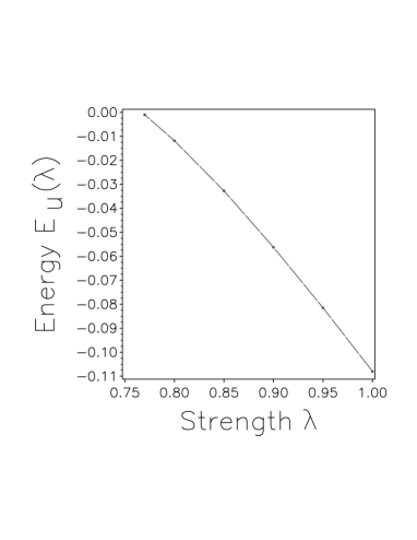
Figure 1: The energy $E_{u}$, defined in the text, as a function of the strength $\lambda$ of the Unitary interaction (7). The energy of the three-boson system would be $E_{T}=-E_{u}(\lambda)\times\Lambda^{2}$. The calculated values are indicated by points and connected by lines for clarity.

Fig. 2 shows the energy as a function of $1/a$ for three chosen values of effective ranges $r_{0}$. One notices a very strong dependence on the effective range.

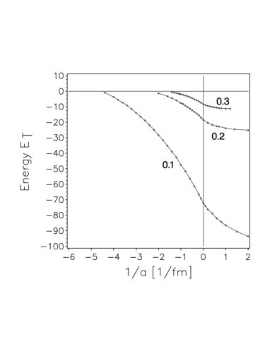
Figure 2: The energy of the three-boson system is shown as a function of the scattering length and three effective ranges that are the parameters defining the 2-body interaction as described in the text. The calculated values are indicated by points and connected by lines for clarity.

Fig. 3 shows energies $E_{T}$ as a function of cut-off $\Lambda$ for $1/a=0$ and some selected values of effective ranges $r_{0}$. It was shown above that for $1/a=0$ and $r_{0}=0$, i.e. the Unitary limit , $E_{T}=0.108\Lambda^{2}$. This is shown numerically by the curve labelled ”.0”. The figure shows that the convergence with $\Lambda$ improves as the effective-range is increased. The value of $\Lambda=\Lambda_{c}$ at which the asymptotic value is reached scales roughly as $10/r_{0}$.

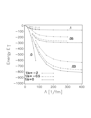
Figure 3: The energy $E_{T}$ of the three-boson system is shown as a function of momentum cut-off $\Lambda$ for three different values of scattering lenghts and four different effective ranges as indicated. See text for further discussion. The calculated values are indicated by points and connected by lines for clarity.

The size of the three-boson system in momentum-space scales roughly the same, consistent with that the size in coordinate space would be $\approx r_{0}$. Fig. 4 shows the rms radius $R_{rms}$ of the $\xi(q)$ function. It follows

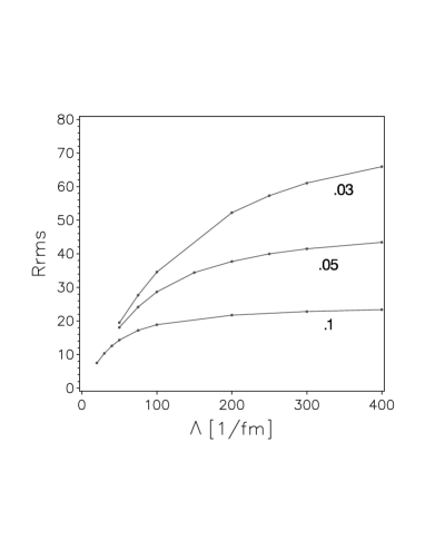
Figure 4: The ’size’ of the three-boson system in momentum-space is shown as a function of cut-off $\Lambda$ for the same effective ranges as in Fig. 3. Only the results for $1/a=0$ are shown. Note the similar $\Lambda$-dependence as is exhibited in Fig. 3. The calculated values are indicated by points and connected by lines for clarity.

closely the $\Lambda$-dependence of $E_{T}$ shown in Fig. 3. One concludes that the size of the system (in momentum-space) determines the minimum range $\Lambda_{c}$ of momenta that the interaction has to span. This is analogous to the situation found in nuclear matter Brueckner calculations where the minimum cut-off is found to be $2k_{f}$ i.e. twice the fermi-momemtum. [9] In the present work on the three-boson system we also find, quite naturally, that $R_{rms}$ is inversely proportinal to $r_{0}$. This is a difference from the Brueckner calculations where the effect of correlations on the momentum distribution is ignored and approximated by the non-interacting fermi-distribution. This is an approximation related to the quasi-particle approximation which is implicit in the Brueckner method. The Green’s function approach goes beyond this approximation including the finite width of the spectral-functions and the momentum-distribution is then wider.

3.2 Rank-2 potential in Unitary Limit

The renormalisation of the non-relativstic three-body problem with short ranged forces was addressed by Bedaque et al[16]. As shown above, the three-boson system with the two-body unitary interaction (7) collapses as $\Lambda^{2}$. Bedaque et al suggests to introduce a three-body counterterm for the renormalisation. One may alternatively choose to introduce a similar counterterm by changing the off-shell two-body t-matrix. As alreday announced in Sect 2 this is done by replacing the rank-1 by a rank-2 interaction with $V_{1}$ chosen so as to modify the short-ranged, ultraviolet, part of the interaction in order to prevent the collapse. With $\delta{k}=-r_{c}*k$ the related potential $V_{1}$ is obtained by inverse scattering. Fig. 5 shows the three-boson energy as a function of cut-off $\Lambda$ for three different values of $r_{c}$. The lowest curve is for $r_{c}=0$ i.e. the rank-1 potential and shows the $\Lambda^{2}$ divergence. The upper five curves are for increasing values of $r_{c}$ as shown in the figure caption. A drastic change is seen with $r_{c}=0.12$ showing convergence for large $\Lambda$.

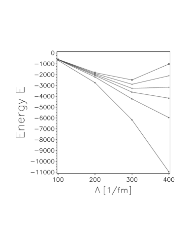
Figure 5: The three-boson energy as a fuction of $\Lambda$ for different values of $r_{c}$. From bottom and up: $r_{c}=0,.001,.0012,.0013,.0014.,0015$ [$fm$]. The calculated values are indicated by dots, connected by straight lines.

3.3 Efimov States

There are many publications related to the low-bound excited states found as solutions of the Faddeev equations, states first discoverd by and named after Vitali Efimov[2] Numerous calculations were done at and close to the unitary limit. Never was found more than one state that could be identified as an ’Efimov’ state although eq. (11) suggests several states should be found with $1/a=r_{0}\sim 0$. The search for these states was in general very elusive and in particular very sensitive to very small changes in the low momenta part of the interactions. The broken curve in Fig. 6 shows the excited state energy $E_{u}(\lambda)$ obtained from solving eq. (9). The solid line represents thw two-body bound state energy. The sole Efimov state is seen to coincide with the two-body at $\lambda=1.08$. The Faddeev equation also yields numerous three-boson energies located above the two-body curve. These represent dimers, two bound bosons, and a free boson. The ground state energies are some fifty times deeper.

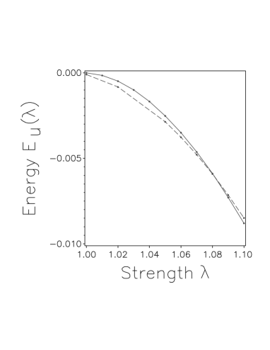
Figure 6: The broken line shows the Efimov state as a function of the strength $\lambda$ of the unitary interaction (7). The energy $E_{u}$ is given in units of $\Lambda^{2}$ as in eq. (9). The full line shows the two-body bound state energy.

Another example is shown in Fig. 7. The separable interaction is here defined by a rank-1 potential with scattering length $a=-2$ and an effective range $r_{0}=.03$. Solutions of the Faddeev equation are shown as a function of the strength multiplier $\lambda$. The solid line shows the two-boson bound state energies.(Not clearly shown is that they are unbound for $\lambda<1.04).$ The sole line below this is the Efimov state. The numerous lines above are dimer+1 states.

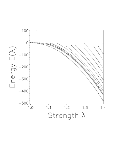
Figure 7: Energies as a function of the strength $\lambda$. The solid line shows the two-boson bound state energies. The sole line below this is the Efimov state. The numerous lines above are dimer+1 states and would not be classified as Efimov states.

Yet another example of the numerous calculations that were made is shown in Fig. 8. The effective range is here $r_{0}=0.1$ and the scattering length is allowed to vary over the range indicated. The dots connected with broken lines indicate solutions of Faddeev equations with the binding energy $E_{B}$ from eq. (6). According to other works these should with incresing $1/a$ approach the bound dimer line. This is not the case here. This may be a characteristic of the separable interaction. Humberston et al [17] show a comparison of separable (non-local) and local (Yukawa and exponential) interactions used in three-boson calculations. The energy increases much faster with the strength of the interaction for the separable than it does for the local interaction. In order to investigate the effect of the binding, another set of calculations were made shown by the broken line connecting squares. Here $E_{B}$ is set to zero in eq. (5). It does have a $1/a$ dependence similar to what was expected from the literature. Only one Efimov state is found here with $r_{0}=0.1$. From eq. (11) 2 states could be expected only for $1/a<.025$. It should be mentioned that expression (11) was tested by Huber [18]. Our result may be associated with the rank-1 potential.

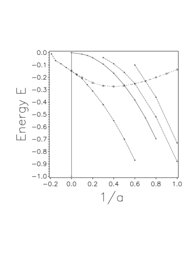
Figure 8: The energy as a function of $1/a$ ($a$ is scattering length) with $r_{0}=0.1$. The solid line shows the dimer bound state energy. The broken lines below this line show Efimov state energies, while those above are dimer+1 energies. The cut-off parameter is here $\Lambda=75$. (Cf Fig. 3). See text for further details. int

4 Summary and Comments

Fig. 2 shows that the energy of the bound system of three-bosons depend strongly on the range $r_{0}$ of the two-body interaction. This is consistent with earlier results for the infinite fermion-system.[8, 15] Fig. 3 shows that as a function of the momentum cut-off $\Lambda$, the energies converge toward asymptotic values $E_{T}$ that, as in Fig.2, are functions of the range $.03<r_{0}<.1$ but largely independent of the scattering length for $|a|\gg r_{0}$. Convergence was reached at $\Lambda_{c}\sim 10/r_{0}\sim 5\times R_{rms}$. The size of the trimer at equilibrium (saturation), the inverse of $R_{rms}$ scales as $r_{0}$ and the range $\Lambda$ has to scale with $R_{rms}$ consistent with our results.

For comparison the curve labelled by ”.0” in Fig. 3 shows the energy vs $\Lambda$ in the unitary limit. As shown above (eq. (9)) this limit has to be treated as a special case giving the analytic result $E_{T}=E_{u}(\lambda)\Lambda^{2}$. The numerical result shown by Fig. 1 is $E_{u}(\lambda=1)=-0.108$ while $E_{u}(\lambda)=0$ for $\lambda\sim 0.77$.

The quadratic divergence and simaltaneous collapse of the boson trimer in the Unitary limit was dampend by a renormalisation procedure consisting of a counter-term represented by a rank-2 potential with results shown in Fig. 5.

Efimov states were identified although not quite as expected which may be a consquence of the specific interactions.

References

- [1] L.D. Faddeev, Zh. Eksperim. Teor. Fiz. 39 (1960) 1459; Sov. Phys. JETP(transl.) 12 (1961) 1014.
- [2] V. Efimov, Phys. Lett. B33 (1970) 903.
- [3] H.D. Amado and J.V. Noble, Phys. Rev. D 5 (1972) 1992.
- [4] M.G. Fuda, Nucl.Phys. A116 (1968) 83.
- [5] R.W. Stagat, Nucl.Phys. A125 (1969) 654.
- [6] Frank Tabakin, Phys. Rev. 177 (1969) 1443.
- [7] N.H. Kwong and H.S. Köhler, Phys. Rev. C 55 (1997) 1650.
- [8] H.S. Köhler , nucl-th/0705.0944.
- [9] H.S. Köhler , nucl-th/0511030.
- [10] H.S. Köhler , nucl-th/0907.1539.
- [11] H.S. Köhler , nucl-th/1008.3884.
- [12] K. Chadan, Nuovo Cimento 10 (1958) 892; Nuovo Cimento A 47 (1967) 510.
- [13] H. Fiedeldey, Nucl.Phys. A 135 (1969) 353.
- [14] H.S. Köhler and S.A. Moszkowki, nucl-th/0703093.
- [15] H.S. Köhler , nucl-th/0801.1123.
- [16] P.F. Bedaque, H.-W. Hammer,U. van Kolck, Nucl. Phys. A646 (1999) 444.
- [17] J.W. Humberston, R.L. Hall and T.A.Osborn Phys. Lett. 27B (1968) 195.
- [18] Stephen Huber, Phys. Rev. a 31 (1985) 3981.