Generalized Bose-Einstein Condensation

Abstract

Generalized Bose-Einstein condensation (GBEC) involves condensates appearing simultaneously in multiple states. We review examples of the three types in an ideal Bose gas with different geometries. In Type I there is a discrete number of quantum states each having macroscopic occupation; Type II has condensation into a continuous band of states, with each state having macroscopic occupation; in Type III each state is microscopically occupied while the entire condensate band is macroscopically occupied. We begin by discussing Type I or “normal” BEC into a single state for an isotropic harmonic oscillator potential. Other geometries and external potentials are then considered: the “channel” potential (harmonic in one dimension and hard-wall in the other), which displays Type II, the “cigar trap” (anisotropic harmonic potential), and the “Casimir prism” (an elongated box), the latter two having Type III condensations. General box geometries are considered in an appendix. We particularly focus on the cigar trap, which Van Druten and Ketterle first showed had a two-step condensation: a GBEC into a band of states at a temperature $T_{c}$ and another “one-dimensional” transition at a lower temperature $T_{1}$ into the ground state. In a thermodynamic limit in which the ratio of the dimensions of the anisotropic harmonic trap is kept fixed, $T_{1}$ merges with the upper transition, which then becomes a normal BEC. However, in the thermodynamic limit of Beau and Zagrebnov, in which the ratio of the boundary lengths increases exponentially, $T_{1}$ becomes fixed at the temperature of a true Type I phase transition. The effects of interactions on GBEC are discussed and we show that there is evidence that Type III condensation may have been observed in the cigar trap.

I Introduction

Bose-Einstein condensation (BEC) has been intensely researched in recent years since the advent of laser and magnetic cooling of trapped alkaline atoms achieved that state Ketterle1 ; Stringari ; Leggett ; PethickSmith . In normal Bose-Einstein condensation (NBEC) a macroscopic number of particles populates a single quantum state (usually the ground state of the system) below a critical temperature. The state is often the lowest momentum state in a homogeneous system Einstein ; London ; Ziff (for an extensive review see Ref. Ziff ), or it could be the lowest harmonic oscillator state in a trapped gas. Many authors have considered alternative possibilities: for example, a number of states may simultaneously be macroscopically occupied, or a band of states is macroscopically occupied while no single state has a macroscopic number of particles. Either of these last two cases is called a “generalized Bose-Einstein condensation” (GBEC). The terminology “generalized” was first used by Girardeau Girar1 ; Girar2 ; Girar3 in considering a homogeneous interacting gas. (See also the work of Luban Luban ). An early description of the phenomenon was by Casimir Casimir in treating a uniform gas in an elongated box (the “Casimir prism”). Rehr and Mermin RehrMermin found that a rotating Bose gas had a GBEC. Other terminology has referred to “smeared” Girar1 and “fragmented” condensations Nozieres1 ; Nozieres2 . The most thorough analyses of GBEC have been done by Van den Berg and coworkers VDB80 ; VDB81 ; VDB82 ; VDB82A ; Pule ; VDB83 ; VDB84 ; VDB86 ; VDB86A and more recently by Zagrebnov et al Zag98-1Int ; Zag98-2Int ; Zag98-3Int ; Zag2000Int ; Zag2000-1Int ; Zag2004 ; Zag08Int ; BeauZag ; Beau . Ho and Yip Ho claim that the spin-1 Bose gas is an example of fragmentation.

However, there seem to be several schools of research on this topic who do not know of and do not quote the others’ work. For example, Van Druten and Ketterle VDK and more recently Beau and Zagrebnov BeauZag have theoretically discussed an example of GBEC. Ref. BeauZag has followed on the extensive work of the Van den Berg group and does not quote Ref. VDK . On the other hand, Ref. VDK , and many references in the literature to this paper, do not refer to the previous papers of the Van den Berg or Zagrebnov schools. A frequently quoted paper by Nozieres Nozieres2 presents a proof to show that fragmented BEC is ruled out for repulsive interacting systems; however, the proof holds only for one kind of GBEC; no proof or reference appears for the other kinds of GBEC. Thus we believe a pedagogic review of the subject is needed, to clarify the subject, make the details more widely known, and perhaps to stimulate experimental research to find cases of the phenomenon.

Van den Berg et al VDB82A have classified three general forms of BEC: There is condensation into

I) a discrete number of quantum states each having macroscopic occupation (of order $N$, the number of particles)—e.g., NBEC has a single condensed state;

II) a band of states with each state having macroscopic occupation.

III) a band of states each state having only microscopic occupation (the occupation number $n_{i}$ of each such state has $n_{i}/N\rightarrow 0$ in the thermodynamic limit), but with the entire band having a macroscopic number of particles.

We will present examples of each of these situations in the present paper. All of our examples will be of ideal gases. The question then arises whether a GBEC can be maintained in the case of interacting systems. Noziéres Nozieres2 showed that interactions would favor NBEC when there were repulsive interactions. Nevertheless there are several cases in the literature where interacting cases of GBEC have been given; we will discuss these later and how they avoid violating the Noziéres analysis.

The treatments of Refs. BeauZag and VDK are interesting in that they bear on BEC in ultra-cold gases; they have theoretically discussed a case of two-step GBEC with a first transition into the lowest band of states in a “cigar”-shaped harmonic trap followed at a lower temperature by a condensation into the lowest single-particle state. The latter transition, into a single state, occurred at a transition temperature $\sim 1/\ln(N)$, which would seem to disappear in the thermodynamic limit (TL). Each pair of authors considers an alternative TL in which the lower transition persists for large particle number. We will discuss these cases more fully below. Sonin Sonin was the first to note that there could be multiple BEC transitions in a parallelepiped geometry corresponding to a variety of way of taking the TL, although he did not discuss any associated GBEC. The original case of a GBEC associated with the double BEC transition was considered by Van den Berg and coworkers in a flat-plate geometry VDB83 ; VDB86 . There have been many experiments with gases in cigar traps; we comment on their relevance to the possible observation of GBEC.

We begin by discussing the normal BEC (NBEC) for an isotropic harmonic potential followed by a sample of Type II condensation. Then we give a detailed discussion of the anisotropic harmonic “cigar” trap, for which transitions are possible at two different temperatures. As discussed above the nature of the lower transition depends crucially on how the TL is taken. Such a result shows a secondary purpose of our paper: to show there is more than one way to go to the large-scale limit; the density of states will depend on the relative values of the respective dimensions of an ansiotropic container. We treat the “Casimir prism” to illustrate GBEC with box boundary conditions in all directions. The effects of interactions on GBEC and the implications of recent experiments are discussed in Sec. VI. A more abstract analysis of the three kinds of GBEC is given in the Appendix.

II The isotropic 3D oscillator

To illustrate NBEC, we use the three-dimensional (3D) isotropic oscillator potential rather than the usual 3D homogeneous ideal gas, because it can show a very interesting GBEC when the potential is made anisotropic. The harmonic potential is taken to be

$$V=\frac{1}{2}\frac{U}{L^{2}}\left(x^{2}+y^{2}+z^{2}\right),$$ (1)

where $U$ is the potential strength. Note that the harmonic potential has been written so it has an evident length scale $L$ and the frequency is

$$\omega=\sqrt{\frac{U}{m}}\frac{1}{L},$$ (2)

where $m$ is the particle mass. We insert this length since taking the thermodynamic limit in a harmonic potential involves increasing the number of particles while weakening the potential to maintain constant overall density $\rho$. Having this length scale is also necessary to see the relative sizes of the occupation numbers of various states Damle ; WJM1D3D . The harmonic length $a_{0}=\sqrt{\hbar/(m\omega)}$ is a measure of the rms deviation of a particle from the center of the well and is not the appropriate density length scale as we will see. The energy levels are

$$\varepsilon_{p_{x}p_{y}p_{z}}=\hbar\omega\left(p_{x}+p_{y}+p_{z}+\frac{3}{2}\right),$$ (3)

with $p_{i}$ taken over all positive integers.

The total number of particles in the system is given in terms of the usual Bose distribution function as

$$N=\sum_{p_{x},p_{y},p_{z}}\left\{\exp\left[\beta\left(\hbar\omega\left(p_{x}+p_{y}+p_{z}\right)-\mu\right)\right]-1\right\}^{-1},$$ (4)

where $\beta=1/(k_{B}T)$ with $T$ the temperature, $k_{B}$ the Boltzmann constant, and $\mu$ the chemical potential. We will always consider the ground-state energy to be incorporated into the chemical potential $\mu$ so that the ground state is effectively zero. We introduce a temperature parameter

$$T_{0}\equiv\frac{\hbar}{k_{B}}\sqrt{\frac{U}{m}}\frac{1}{a},$$ (5)

where $a=1/\rho^{1/3}$ is an average interparticle separation.

For high temperature $T$ we can replace the sums by integrals:

$$N = \int_{0}^{\infty}dp_{x}\int_{0}^{\infty}dp_{y}\int_{0}^{\infty}dp_{z}\frac{1}{\exp\left[\frac{T_{0}a}{TL}\left(p_{x}+p_{y}+p_{z}\right)-\beta\mu\right]-1}$$ (6)

$$= \frac{L^{3}}{a^{3}}\left(\frac{T}{T_{0}}\right)^{3}\int_{0}^{\infty}du_{1}\int_{0}^{\infty}du_{2}\int_{0}^{\infty}du_{3}\frac{1}{e^{\left(u_{1}+u_{2}+u_{3}+\alpha\right)}-1},$$

where $u_{i}=T_{0}ap_{i}/TL$ and

$$\alpha = -\beta\mu.$$ (7)

The integral is most easily done by expanding the integrand in inverse powers of the exponential to get

$$N = \frac{L^{3}}{a^{3}}\left(\frac{T}{T_{0}}\right)^{3}\int_{0}^{\infty}du_{1}\int_{0}^{\infty}du_{2}\int_{0}^{\infty}du_{3}\sum_{l=1}^{\infty}e^{-l\left(u_{1}+u_{2}+u_{3}+\alpha\right)}$$ (8)

$$= \frac{L^{3}}{a^{3}}\left(\frac{T}{T_{0}}\right)^{3}F_{3}(\alpha),$$

where the Bose integral Robinson is

$$F_{n}(\alpha)\equiv\sum_{l=1}^{\infty}\frac{e^{-l\alpha}}{l^{n}}.$$ (9)

We see that the way to define a density parameter (or any thermodynamic variable) so that it is scale independent Damle ; WJM1D3D is in terms of a volume $L^{3}$ with the parameter given by

$$\rho=\frac{1}{a^{3}}=\frac{N}{L^{3}}.$$ (10)

As the temperature decreases, Eq. (8) can be satisfied by decreasing $\alpha$ until the quantity $F_{3}(\alpha)$ has a maximum, $F_{3}(0)=\zeta(3)=1.202$ where $\zeta(n)$ is the Riemann zeta function. The temperature corresponding to this maximum is the critical temperature $T_{c}$ given by

$$T_{c}=\frac{T_{0}}{\zeta(3)^{1/3}}.$$ (11)

Below the transition temperature the non-condensed particle number, $N-N_{0},$ with $N_{0}$ the condensate number, is still given by the right side of Eq. (8) with $\alpha=0:$

$$N-N_{0} = \frac{L^{3}}{a^{3}}\left(\frac{T}{T_{0}}\right)^{3}\zeta(3)$$ (12)

$$= N\left(\frac{T}{T_{c}}\right)^{3},$$

from which we see that

$$N_{0}=N\left[1-\left(\frac{T}{T_{c}}\right)^{3}\right].$$ (13)

Assume that all the condensed particles fall into the ground state (as usual); the occupation number corresponding to the ground state is

$$n_{000} = \frac{1}{e^{\alpha}-1}$$ (14)

$$\approx \frac{1}{\alpha}=N_{0}=O\left(\frac{L^{3}}{a^{3}}\right),$$

where $O(x)$ means order of magnitude of $x$. Thus $\alpha$ is small, but not actually zero. The low excited states have occupation

$$n_{p_{x}p_{y}p_{z}} = \left\{\exp\left[\frac{T_{0}a}{TL}(p_{x}+p_{y}+p_{z})+\alpha\right]-1\right\}^{-1}$$ (15)

$$\approx \left[\frac{T_{0}a}{TL}(p_{x}+p_{y}+p_{z})+\alpha\right]^{-1}.$$

Since $\alpha$ is so small we can drop that term in Eq. (15) as long as some $p_{i}>0$. In that case the occupation number is $O(L/a)=O(N^{1/3}),$ which is small relative to the ground-state occupation, $O(N)$. Only the ground state is macroscopically occupied. All this is quite standard except here we have states of an oscillator potential rather than free particles in a box. The BEC considered here is Type I because only one state has macroscopic occupation.

Normal BEC might also include cases where there are a discrete number of states each having macroscopic occupation. For example, the well-know experiment MITInterf in which two condensates were brought together to form an interference pattern is such an example. One might also consider multiple condensates each having a different spin orientation Ho ; LMSpinLetter . Condensates trapped in multiple wells are sometimes said to be “fragmented” Alon .

III The channel potential

In a Type II condensation we have a band of states each with macroscopic occupation. Here we discuss a rather peculiar case VDB81 in which a spinless two-dimensional (2D) ideal gas has a harmonic potential in the $z$ direction and is free in the $x$ direction with periodic boundary conditions in that direction over a large distance $L$. The potential forms what might be called a channel or trough. The energy levels are

$$\varepsilon_{k_{x}p_{z}}=\frac{\hbar^{2}k_{x}^{2}}{2m}+\hbar\omega\left(p_{z}+\frac{1}{2}\right),$$ (16)

with the harmonic frequency given by Eq. (2); we use the same $L$ parameter in both momentum and harmonic dimensions. The total number of particles in the system is given in terms of the usual Bose distribution function as

$$N=\sum_{s_{x},p_{z}}\left\{\exp\left[\beta\left(\frac{h^{2}s_{x}^{2}}{2mL^{2}}+\hbar\sqrt{\frac{U}{m}}\frac{p_{z}}{L}-\mu\right)\right]-1\right\}^{-1}$$ (17)

with $s_{x}=0,\pm 1,\pm 2\cdots$ . We define two temperature parameters

$$T_{x}=\frac{h^{2}}{k_{B}2ma^{2}}$$ (18)

and

$$T_{z}=\frac{\hbar}{k_{B}}\sqrt{\frac{U}{m}}\frac{1}{a},$$ (19)

where the density is $\rho=1/a^{2}$. These temperatures are simply natural units expressed in terms of the parameters of the problem. For simplicity we assume the two parameters are the same: $T_{x}=T_{z}\equiv T_{0}$. For high temperature $T$ we can change the sums to integrals:

$$N = \int_{-\infty}^{\infty}ds_{x}\int_{0}^{\infty}dp_{z}\frac{1}{\exp\left[\frac{T_{0}a^{2}}{TL^{2}}s_{x}^{2}+\frac{T_{0}a}{TL}p_{z}-\beta\mu\right]-1}$$ (20)

$$= \frac{L^{2}}{a^{2}}\left(\frac{T}{T_{0}}\right)^{3/2}\int_{-\infty}^{\infty}du\int_{0}^{\infty}dw\frac{1}{e^{\left(u^{2}+w+\alpha\right)}-1}$$

$$= N\left(\frac{T}{T_{0}}\right)^{3/2}\sqrt{\pi}F_{3/2}(\alpha),$$

since the average density is $\rho=N/L^{2}$. $F_{3/2}(\alpha)$ has a maximum $\zeta(3/2)=2.61$ (as in the standard 3D homogeneous gas). The critical temperature is

$$T_{c}=T_{0}\left(\frac{1}{\sqrt{\pi}\zeta(3/2)}\right)^{2/3}.$$ (21)

For $T<T_{c}$ there is a condensate whose number $N_{0}$ is given by

$$N-N_{0} = N\left(\frac{T}{T_{0}}\right)^{3/2}\sqrt{\pi}F_{3/2}(0)$$ (22)

$$= N\left(\frac{T}{T_{c}}\right)^{3/2},$$

or the condensate fraction $f_{0}=N_{0}/N$ is

$$f_{0}=\left[1-\left(\frac{T}{T_{c}}\right)^{3/2}\right].$$ (23)

Assume that the ground state (that is, lowest $k-$state of the lowest harmonic level $p_{z}=0$) is macroscopically occupied with number

$$n_{00} = \frac{1}{e^{\alpha}-1}$$ (24)

$$\approx \frac{1}{\alpha}=O\left(\frac{L^{2}}{a^{2}}\right).$$

However, now the excited states cannot be neglected as in Sec. II. Consider the entire band of $k$ states corresponding to the lowest harmonic level $p_{z}=0$. The low excited states have occupation

$$n_{s_{x},0}\approx\left[\beta\left(\frac{h^{2}s_{x}^{2}}{2mL^{2}}\right)+\frac{a^{2}\gamma}{L^{2}}\right]^{-1},$$ (25)

where we have written $\gamma=\alpha L^{2}/a^{2}$. Obviously $n_{s_{x},0}=O(L^{2}/a^{2})$ for all $k$. On the other hand, we can easily see that the harmonic bands of states with $p_{z}>0$ do not contribute macroscopically, being of order $L/a\ll N.$ We must sum up the contribution $N_{b}$ of the first harmonic band ($p_{z}=0)$. We then have for the band number

$$N_{0}=N_{b} \equiv \sum_{s_{x}=-\infty}^{\infty}\frac{1}{\exp\left[\frac{1}{N}\left(\frac{T_{0}}{T}s_{x}^{2}+\gamma\right)\right]-1}$$ (26)

$$\cong \sum_{s_{x}=-\infty}^{\infty}\frac{1}{\left[\frac{1}{N}\left(\frac{T_{0}}{T}s_{x}^{2}+\gamma\right)\right]}$$

$$= N\pi\sqrt{\frac{T}{T_{0}\gamma}}\coth\left(\pi\sqrt{\frac{T\gamma}{T_{0}}}\right).$$

The sum in the last line is exact; replacing the sum in the first line by an integral is not sufficiently accurate for all $T$ (it sets the coth factor equal to one). Setting the temperature dependent result found in Eq. (23) to $N_{b}/N$ from Eq. (26) gives us an equation for $\gamma$, which can be used to evaluate the individual energy-state occupation fractions $n_{s_{x},0}/N$. The results are shown in Fig. 1.

Figure 1: The condensate distributions for the channel potential versus temperature. The solid line is the entire condensate distribution $f_{0};$ the dashed line is the that of the lowest momentum state $f_{0,0}=n_{0,0}/N$ of the condensate band; the dotted lines are the distributions of the next higher momentum levels.

Near the condensation temperature the number of macroscopic states involved is clearly very large. Only near $T=0$ does the lowest state become dominant. All these occupation numbers are of order $N.$

IV The Cigar Trap

For another, and most detailed, example of GBEC we consider the anisotropic harmonic trap. A few years ago Van Druten and Ketterle (VDK) VDK suggested an unusual BEC that would take place in a cigar-shaped harmonic trap (one long dimension with a weak harmonic potential, plus two short dimensions with much stronger transverse potentials). More recently Beau and Zagrebnov (BZ) BeauZag independently treated the same problem. In each treatment there is a GBEC into a band of states, and a second transition at a lower temperature. In these treatments we learn that there are two ways to take the thermodynamic limit (TL); in one the transition disappears (that is, it is a pseudo-transition), while in the other it persists in the infinitely large system. This peculiarity illustrates some interesting unexpected features of the statistical mechanics of BEC. The approach used by BZ to fix this second transition was originally invented by Van den Berg and co-workers VDB83 ; VDB86 for an anisotropic square well potential.

The energy levels of the cigar trap are

$$\varepsilon_{p_{x}p_{y}p_{z}}=\hbar\omega_{\perp}(p_{x}+p_{y})+\hbar\omega_{\|}p_{z},$$ (27)

where $\omega_{i}=\sqrt{U/m}/L_{i}$ corresponding to the two lengths $L_{\perp}$ and $L_{\|}$, with $L_{\|}\gg L_{\perp}$. The density parameter of the gas is then taken to be

$$\rho=\frac{N}{L_{\perp}^{2}L_{\|}}.$$ (28)

We again define a characteristic temperature $T_{0}$ just as in Eq. (5). With this notation the particle number must satisfy

$$N=\sum_{p_{x},p_{y},p_{z}}\frac{1}{\exp\left[\frac{T_{0}a}{T}\left(\frac{p_{x}+p_{y}}{L_{\perp}}+\frac{p_{z}}{L_{\|}}\right)+\alpha\right]-1}.$$ (29)

Change the sum to an integral for $T$ large to give

$$N = \int_{0}^{\infty}dp_{x}\int_{0}^{\infty}dp_{y}\int_{0}^{\infty}dp_{z}\frac{1}{\exp\left[\frac{T_{0}a}{T}\left(\frac{p_{x}+p_{y}}{L_{\perp}}+\frac{p_{z}}{L_{\|}}\right)+\alpha\right]-1}$$ (30)

$$= \left(\frac{T}{T_{0}}\right)^{3}\frac{L_{\perp}^{2}L_{\|}}{a^{3}}\int_{0}^{\infty}du\int_{0}^{\infty}dv\int_{0}^{\infty}dw\frac{1}{\exp\left[u+v+w+\alpha\right]-1}$$

$$= \left(\frac{T}{T_{0}}\right)^{3}N\sum_{l=1}^{\infty}e^{-\alpha l}\int_{0}^{\infty}du\int_{0}^{\infty}dv\int_{0}^{\infty}dwe^{-l(u+v+w)}$$

$$= \left(\frac{T}{T_{0}}\right)^{3}N\sum_{l=1}^{\infty}\frac{e^{-\alpha l}}{l^{3}}=N\left(\frac{T}{T_{0}}\right)^{3}F_{3}(\alpha).$$

Thus the chemical potential parameter $\alpha$ has to satisfy

$$\left(\frac{T}{T_{0}}\right)^{3}F_{3}(\alpha)=1.$$ (31)

If $T$ becomes too small, the equation can no longer be satisfied. The condensation temperature is

$$T_{c} = \frac{T_{0}}{\zeta(3)^{1/3}}$$ (32)

$$= \frac{\hbar}{k_{B}}\sqrt{\frac{U}{m}}\left(\frac{\rho}{\zeta(3)}\right)^{1/3},$$

where the density $\rho$ is given by Eq. (28).

The number of noncondensate particles now satisfies the relation

$$N-N_{0}=N\left(\frac{T}{T_{c}}\right)^{3},$$ (33)

with $N_{0}$ the condensate number or

$$f_{0}(T)\equiv\frac{N_{0}}{N}=1-\left(\frac{T}{T_{c}}\right)^{3}.$$ (34)

When the temperature is below $T_{c}$ the condensation is in a band of states, as we will show explicitly below. The band occupation number is

$$N_{b} = \sum_{p_{z}=0}^{\infty}\frac{1}{\exp\left[\frac{T_{0}a}{T}\frac{p_{z}}{L_{\|}}+\alpha\right]-1}.$$ (35)

If we change the sum to an integral we find

$$N_{b} = \frac{TN}{T_{0}K}\int_{0}^{\infty}dw\frac{1}{\exp\left[w+\alpha\right]-1},$$ (36)

in which we have made the substitution

$$\frac{L_{\|}}{a}=\left(\frac{N}{L_{\perp}^{2}L_{\|}}\right)^{1/3}L_{\|}=\frac{N}{K},$$

where

$$K\equiv\left(N\frac{L_{\perp}}{L_{\|}}\right)^{2/3}.$$ (37)

Note the assumption (to be corrected later) in this replacement of the sum by an integral, that the ground state occupation remains as small as that of the rest of the states. Carrying out the integration gives

$$f_{b}\equiv\frac{N_{b}}{N}=-\frac{T}{T_{0}K}\ln\left(1-e^{-\alpha}\right).$$ (38)

If indeed the ground-state occupation is negligible, then the band occupation is the whole condensate, $f_{b}=f_{0}$ and, since $\alpha$ is very small below the transition temperature, we have $\ln(1-e^{-\alpha})\approx\ln\alpha$; we can solve for $\alpha$ to find

$$\alpha=e^{-f_{0}\frac{T_{0}}{T}K}.$$ (39)

The band states are analogous to a one-dimensional (1D) gas of Bose particles in the long harmonic trap. Does this 1D gas also have its own condensation into its lowest-energy state, which is, of course, the overall ground state? Subsequent treatment now depends on the boundary conditions used in taking the TL.

IV.1 Standard boundary conditions

Under normal thermodynamic limit conditions, the ratio

$$\Delta\equiv\frac{L_{\|}}{L_{\perp}}$$ (40)

is held constant, while $N,L_{\|,}$ and $L_{\perp}$ are increased. In the present TL, $K=\left(N/\Delta\right)^{2/3}$ (Eq. (37)) would be increasingly large as $N$ increases ($\sim N^{2/3})$ and, for $T\lesssim T_{c}$, $\alpha$ would be increasingly small going as $\alpha\sim e^{-N^{2/3}}$from Eq. (39).

The occupation numbers of the low-lying band levels are

$$n_{00p_{z}}\cong\frac{1}{\frac{T_{0}K}{T}\frac{p_{z}}{N}+\alpha}.$$ (41)

The first term in the denominator being of order $N^{-1/3}$ dominates $\alpha$ giving $n_{00p_{z}}=O(N^{1/3})$ and $n_{00p_{z}}/N\rightarrow 0$ in the TL (microscopic occupation); the condensation is then of Type III as listed in Sec. I. The $p_{z}=0$ term is the exception; when $n_{000}/N$ is microscopic, the condensation remains of Type III. However, the ground state occupation can become $O(N)$ when

$$n_{000}\cong\frac{1}{\alpha}=e^{f_{0}\frac{T_{0}}{T}K}=cN,$$ (42)

where $c\lesssim 1.$ This occurs at a temperature $T_{1}$ given by

$$\frac{T_{1}}{f_{0}(T_{1})}=T_{0}\frac{K}{\ln cN},$$ (43)

or, assuming $N$ large and $T_{1}$ is sufficiently smaller than $T_{c}$ that $f_{0}\approx 1,$ we have

$$T_{1}=\frac{\hbar}{k_{B}}\sqrt{\frac{U}{m}}\frac{N}{L_{\|}\ln N},$$ (44)

which might be considered the condensation temperature of the 1D band. In the TL, $T_{1}$ would go to zero as $1/\ln N$ if the 1D density $N/L_{\|}$ were held constant. Such a behavior is indeed characteristic of a 1D pseudo-phase-transition WJM1D3D ; VDK1D3D , which does not exist except in a finite system. While it is possible to consider a 3D TL such that $L_{\perp}$ is held constant while $N$ and $L_{\|}$ increase, it is $\rho=N/(L_{\perp}^{2}L_{\|})$ and $\Delta$ that are held constant in the standard 3D TL while the two lengths increase. In Eq. (43), when the right side becomes very large, $\sim N^{2/3}/\ln N$, the only way the equation can be satisfied is to have $T_{1}\approx T_{c}$ so that the denominator on the left, $f_{0}(T_{1}),$ almost vanishes (See Eq. (34)). Thus in the TL, $T_{1}\rightarrow T_{c}$ and the “1D” transition coincides with the condensation into the band of states, that is, the band then collapses to just the ground state and the system reverts to the normal BEC rather than a GBEC. Such a result is rather surprising and has not been noted before in the literature. See below for a numerical example.

When the ground state occupation becomes large, the analysis of Eq. (36) is no longer valid, and we need to be a bit more careful to find an expression for the ground-state occupation number. In the sum of Eq. (35) we should split off the ground state term $n_{g}$ to write

$$N_{0} = n_{g}+N_{b}$$ (45)

$$= n_{g}+\sum_{p_{z}^{\prime}=0}^{\infty}\frac{1}{\exp\left[\frac{T_{0}K}{T}\frac{p_{z}^{\prime}}{N}+\alpha^{\prime}\right]-1},$$

where we have redefined the summation index $p_{z}^{\prime}=p_{z}-1$ and let

$$\alpha^{\prime}=\alpha+\frac{T_{0}K}{NT}.$$ (46)

The ground-state occupation fraction is

$$f_{g}=\frac{1}{N\left(e^{\alpha}-1\right)}.$$ (47)

Replace the sum by an integral as before to give

$$f_{0}=\frac{1}{N}\frac{1}{e^{\alpha}-1}-\frac{T}{T_{0}K}\ln\left[1-e^{-\left(\frac{T_{0}K}{NT}+\alpha\right)}\right],$$ (48)

Since the total condensate $f_{0}$ is given by Eq. (34), this is a transcendental equation for $\alpha.$

A formula to solve self-consistently for $f_{g}$ for all situations is gotten from Eq. (48) by solving Eq. (47) for $e^{\alpha}$ in terms of $f_{g}$:

$$f_{g}=f_{0}+\frac{T}{T_{0}K}\ln\left[1-e^{-\frac{T_{0}K}{NT}}\frac{1}{1+1/(Nf_{g})}\right].$$ (49)

In the TL the factor in front of the logarithm in Eq. (49) dominates the behavior and the second term goes to zero so $f_{g}\rightarrow f_{0}$ as we stated above.

IV.2 Numerics

Generally we have

$$\frac{T_{c}}{T_{0}}=\frac{1}{\zeta(3)^{1/3}}=0.94.$$ (50)

VDK considered a set of parameters with $N=10^{6}$ and $\Delta=5.6\times 10^{4}$. In the this case we have

$$K \equiv \left(N\frac{L_{\perp}}{L_{\|}}\right)^{2/3}=\left(\frac{10^{6}}{5.6\times 10^{4}}\right)^{2/3}=6.8,$$ (51)

$$\frac{T_{1}}{T_{c}} = f_{0}(T_{1})\frac{K\zeta(3)^{1/3}}{\ln N}=0.47\quad.$$ (52)

The numerical result in Eq. (52) was gotten by iteration; if we set $f_{0}=1$ in the $T_{1}$ formula we get $T_{1}/T_{c}=0.52$; putting that back on the right in $f_{0}(T_{1})$ gives a new value of $T_{1}$, etc. In Fig. 2 we plot the results for $f_{0}$ and $f_{g}$, where we have solved Eq. (49) by simple iteration.

Figure 2: The condensate distributions in the standard boundary limiting case (the ratio of boundary lengths $\Delta=L_{\|}/L_{\perp}$is a fixed constant) and for $N=10^{6},$ $\Delta=5.6\times 10^{4}$. The solid curve represents the full condensate $f_{0}$ (the fraction of particles in the lowest band of states), while the dotted curve is the ground-state pseudo-condensate $f_{g}$ (the fraction in the lowest state of the lowest band).

In the case where we keep the same length ratio, but increase the number of particles to $N=10^{8}$ we have

$$K = \left(\frac{10^{8}}{5.6\times 10^{4}}\right)^{2/3}=147,$$ (53)

$$\frac{T_{1}}{T_{c}} = \frac{f_{0}(T_{1})K\zeta(3)^{1/3}}{\ln N}=0.961\quad.$$ (54)

Fig. 3 shows the plots of the two condensate fractions for $N=10^{8}$. The ground-state transition almost coincides with the band condensate as expected from the analytic argument.

Figure 3: The condensate distributions in the standard boundary limiting case (the ratio of boundary lengths $\Delta=L_{\|}/L_{\perp}$is a fixed constant) and for $N=10^{8},$ $\Delta=5.6\times 10^{4}$. The solid curve represents the full condensate $f_{0}$, while the dotted curve is the ground-state pseudo-condensate $f_{g}$.

$T_{1}$ approaches $T_{c}$ because in Eq. (43) the right side becomes very large with $K\sim N^{2/3}\rightarrow\infty$, requiring increasingly large $1/f_{0}(T_{1})$ on the left as explained above. The question then arises whether there is a TL such that the right side does not become large, that is, in which $K\sim\ln N$. In the next section we will find such a case.

IV.3 Exponential boundary conditions

Here we consider how the above discussion is changed if we now take the length ratio to obey

$$\Delta=\frac{L_{\|}}{L_{\perp}}=e^{gL_{\perp}^{2}},$$ (55)

a boundary condition that certainly forces the system to become more 1D as $L_{\perp}$ increases. Similar exponential boundary relations were first proposed by Van den Berg and co-workers VDB83 ; VDB86 for an anisotropic square well potential. But these explicit conditions for the anisotropic harmonic oscillator, in which the length factor in the exponent is squared were given by Beau and Zagrebnov BeauZag ; Beau and we designate them as BZ conditions. That they fit the requirement that $K\sim\ln N$ will be verified below. It becomes useful to use a unitless notation here. Let

$$\ell_{\perp} = \rho^{1/3}L_{\perp},$$

$$\ell_{\|} = \rho^{1/3}L_{\|},$$

$$\gamma = \frac{g}{\rho^{2/3}}.$$ (56)

Then, from the density relation Eq. (28), we have

$$N = \ell_{\perp}^{2}\ell_{\|}=\ell_{\perp}^{3}e^{\gamma\ell_{\perp}^{2}}=\ell_{\perp}^{3}\Delta,$$

$$K = \ell_{\perp}^{2},$$

$$\gamma = \frac{\ln\Delta}{\ell_{\perp}^{2}}.$$ (57)

The VDK parameters $N=10^{6}$ and $\Delta=5.6\times 10^{4}$ can be considered a special case (one particular $N$ value) of a BZ set. Then $N$ and $\Delta$ give the corresponding $\gamma$ value. From the above formulas we have $\ell_{\perp}=2.61$ and $\gamma=1.60,$ which is the $\gamma$ value we will use later for larger $N$ values at the same density. For the original VDK parameters, the curves for $f_{0}$ and $f_{g}$ are obviously identical to those shown in Fig. 2; however, with the condition Eq. (55) and a larger $N$ value, $f_{g}$ will no longer merge with the $f_{0}$ as we will see. We consider a much larger $N$ value and solve Eq. (49) for $f_{g}$. We show the comparison of the $f_{g}$ curves for $N=10^{6}$ and $N=10^{16}$ in Fig. 4.

Figure 4: The ground-state condensate distributions $f_{g}$ in the BZ boundary limiting case (the ratio of boundary lengths $L_{\|}/L_{\perp}=e^{gL_{\perp}^{2}}$ is not a fixed constant in the thermodynamic limit). The dotted curve is for $N=10^{6}$ while the solid curve is for $N=10^{16}$.

We can understand the behavior of the large $N$ curve by approximating Eq. (49): For large $N$ (any we have used here) we can expand the exponential and the fraction inside the logarithm to find

$$f_{g}=f_{0}+\frac{T}{T_{0}K}\ln\left[\frac{T_{0}K}{NT}+\frac{1}{Nf_{g}}\right]\approx f_{0}-\frac{T}{T_{0}K}\ln\left[N\right],$$ (58)

where the last approximation holds because $N$ is much larger than the other factors in the logarithm. The parameter $K=\ell_{\perp}^{2}$ can be expressed approximately as well. From Eq. (57) we write

$$\gamma\ell_{\perp}^{2}=\ln N-\frac{3}{2}\ln\ell_{\perp}^{2}.$$ (59)

By iterating this formula once, we see that the second term is much smaller than the first and so

$$K=\ell_{\perp}^{2}\approx\frac{\ln N}{\gamma}.$$ (60)

Putting this in Eq. (58) gives

$$f_{g}(T)=f_{0}(T)-\frac{T\gamma}{T_{c}\zeta(3)^{1/3}}.$$ (61)

We plot this result in comparison with the $N=10^{16}$ result in Fig. 5.

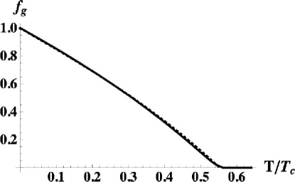
Figure 5: The ground-state condensate distributions $f_{g}$ in the BZ boundary limiting case for $N=10^{16}$ (solid curve) and the thermodynamic limiting value, Eq. (61) (dotted curve).

The lower transition temperature is gotten by setting the left side of Eq. (61) to zero:

$$T_{1}=\frac{T_{c}f_{0}(T_{1})\zeta(3)^{1/3}}{\gamma},$$ (62)

which must be solved self-consistently. We find $T_{1}=0.552T_{c}.$ Clearly this approximation is very good and the system has two distinct phase transitions as BZ have claimed. Perhaps we should not be too surprised that this was possible. In the VDK case having $T_{1}\thickapprox 0.5T_{c}$ was arranged by a judicious choice of $\Delta$ for $N=10^{6}$. The question then is whether it is possible, for a larger value of $N,$ to find a $\Delta$ such that $T_{1}$ and $\rho$ are both unchanged. Such a value is given by Eq. (55). VDK also numerically treated a case in which $T_{1}$ was fixed while $N$ increased, although they did not specify how this was done; they apparently used a form equivalent to Eq. (55).

There is a case of box boundary conditions (square-well potential) that is isomorphic to the harmonic system treated in this section. This is the flat plate geometry in which two large square plates of length $L$ on a side are separated by a much smaller distance $D.$ This problem was treated by Van den Berg and coworkers VDB83 ; VDB86 in the 1980’s. A third analogous case involves having two free dimensions and one harmonic dimension BeauZag .

Sonin Sonin gave an analysis of multi-step quasi-condensations in finite systems for anisotropic free-particle boundary conditions and showed that a second transition could be preserved in the thermodynamic limit by an appropriate thermal limiting procedure. Deng Deng and Shiokawa Shiokawa treated multi-step transitions in finite anisotropic harmonic potentials; the extra transitions disappear in the normal TL.

V GBEC in a box: The Casimir prism

We consider one more Type III GBEC where there is again a macroscopic condensation into a band number of states while the occupation of any single quantum state remains microscopic. With this geometry there is no second transition at a lower temperature. The case considered here was treated by Casimir Casimir and later by others VDB82A ; VDB86 ; Zag2004 ; BeauZag ; Beau . It was one of the first known theoretical cases of GBEC. The geometry is shown in Fig. 6. The length $L$ is much larger than the side $D$ of the square cross section.

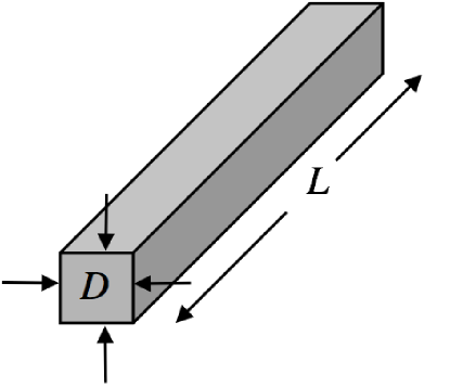
Figure 6: Casimir Prism. A box with one side $L$ much greater than the square end face dimension $D.$

The free-particle states in this system are given by

$$\varepsilon_{s_{x}s_{y}s_{z}}=\frac{h^{2}}{2m}\left[\frac{(s_{x}^{2}+s_{y}^{2})}{D^{2}}+\frac{s_{z}^{2}}{L^{2}}\right],$$ (63)

where the $s_{i}$ are again positive or negative integers. The total number of particles is a sum

$$N=\sum_{s_{x}s_{y}s_{z}}\frac{1}{\exp\left\{\beta\left[\frac{h^{2}}{2m}\left(\frac{(s_{x}^{2}+s_{y}^{2})}{D^{2}}+\frac{s_{z}^{2}}{L^{2}}\right)-\mu\right]\right\}-1}.$$ (64)

Above any transition we can change the sum to an integral:

$$N = \int_{-\infty}^{\infty}ds_{x}\int_{-\infty}^{\infty}ds_{y}\int_{-\infty}^{\infty}ds_{z}\frac{1}{e^{\beta\left[\frac{h^{2}}{2m}\left(\frac{(s_{x}^{2}+s_{y}^{2})}{D^{2}}+\frac{s_{z}^{2}}{L^{2}}\right)-\mu\right]}-1}$$ (65)

$$= \frac{LD^{2}}{h^{3}}\left(\frac{2m}{\beta}\right)^{3/2}\int_{-\infty}^{\infty}du_{1}\int_{-\infty}^{\infty}du_{2}\int_{-\infty}^{\infty}du_{3}\frac{1}{e^{\left(u_{1}^{2}+u_{2}^{2}+u_{3}^{2}+\alpha\right)}-1}$$

$$= \left(\frac{2\pi m}{\beta h^{2}}\right)^{3/2}LD^{2}F_{3/2}(\alpha).$$

$F_{3/2}(\alpha)$ has a maximum of $\zeta(3/2)$ at $\alpha=0$ so the transition temperature is given by

$$T_{c}=\frac{h^{2}}{2\pi mk_{B}}\left(\frac{\rho}{\zeta(3/2)}\right)^{2/3}.$$ (66)

For $T<T_{c}$, Eq. (65) is no longer valid, and below $T_{c}$ the condensed particle number $N_{0}$ satisfies

$$N_{0}=N\left[1-\left(\frac{T}{T_{c}}\right)^{3/2}\right].$$ (67)

Because of the anisotropy of the boundary conditions, a band of states with $s_{x}=0,$ $s{}_{y}=0$ fills at the transition. To see how this occurs, we examine the density of low excited states. There are various ways to take the thermodynamic limit, but here we hold $D$ constant while we take $L\rightarrow\infty$. (The arguments presented here also hold if we let $L,D\rightarrow\infty$ with $L$ approaching infinity faster than $D^{2}.$ Compare with Appendix A.3.) Let us first hypothesize that the ground state is macroscopically occupied so that $\alpha\sim O(1/(D^{2}L))$ (which we will see is incorrect); the occupation of the low states would then be

$$n_{s_{x},s_{y},s_{z}} \approx \frac{1}{\left[\frac{h^{2}\beta}{2m}\left(\frac{(s_{x}^{2}+s_{y}^{2})}{D^{2}}+\frac{s_{z}^{2}}{L^{2}}\right)+\alpha\right]}.$$ (68)

Under our hypothesis, the first term would dominate the other two, which could be dropped and the state density would be $O(1)$ unless $s_{x}=s_{y}=0.$ In that case, the $s_{z}$ term would still be negligible and we would find $n_{0,0,s_{z}}\sim O(N)$ for all values of $s_{z}$. Clearly we need to sum up the entire band of $s_{z}$ states to find the true behavior. The number of particles in the band is

$$N_{b} = \sum_{s_{z}}\frac{1}{\exp\left[\frac{\beta h^{2}}{2m}\frac{s_{z}^{2}}{L^{2}}+\alpha\right]-1}$$ (69)

$$= \left(\frac{2m}{\beta h^{2}}\right)^{1/2}L\int_{-\infty}^{\infty}dw\frac{1}{\exp\left\{w^{2}+\alpha\right\}-1}$$

$$= \left(\frac{2\pi m}{\beta h^{2}}\right)^{1/2}LF_{1/2}(\alpha).$$

Below the transition temperature, $\alpha$ is small and $N_{b}$ equals the condensate number of particles $N_{0}$. Further, since Robinson for small $\alpha$, $F_{1/2}(\alpha)\approx\sqrt{\pi/\alpha}$, one gets

$$N_{0}=\left(\frac{2\pi^{2}m}{\beta h^{2}}\right)^{1/2}\frac{L}{\sqrt{\alpha}}$$ (70)

or

$$\alpha = \frac{2\pi^{2}m}{\beta h^{2}}\left(\frac{L}{N_{0}}\right)^{2}$$ (71)

$$= \frac{2\pi^{2}m}{\beta h^{2}}\frac{1}{\rho_{0}^{2}D^{4}},$$

where $\rho_{0}=N_{0}/LD^{2}$. This result is quite different from what it would have been if the ground state were macroscopically occupied as in our initial hypothesis of $\alpha\sim 1/(D^{2}L)$.

The condensate number is macroscopic, but the numbers in the single-particle states are not. The density corresponding to low quantum numbers $\left\{0,0,s_{z}\right\}$ is

$$\rho_{0,0,s_{z}} \approx \frac{1}{LD^{2}\left[\frac{h^{2}\beta}{2m}\frac{s_{z}^{2}}{L^{2}}+\frac{\gamma(T)}{D^{4}}\right]}$$ (72)

$$= \frac{1}{\left[\frac{h^{2}\beta}{2m}s_{z}^{2}\frac{D^{2}}{L}+\frac{\gamma L}{D^{2}}\right]},$$

where $\gamma=\alpha D^{4}$. The term in $\gamma$ always dominates so the occupation of each of these states is microscopic and approaches zero as $1/L$, including the ground state with $s_{z}=0$. Of course, at $T=0$ the ground state must finally have all the particles in it, but the temperature at which this occurs can be estimated by using $\alpha$ from Eq. (71) in $\rho_{0,0,0}\approx 1/(N\alpha)$ to see that the onset temperature for macroscopic occupation of the ground state is $T\sim T_{c}$$\rho^{1/3}D^{2}/L$, which is zero in the TL or very small in a real experiment.

There is an alternative way to take the limit in which all three dimensions of the box become infinite. This way can also be used to distinguish the three kinds of GBEC. We discuss this in the Appendix.

VI The effects of interactions on GBEC

VI.1 GBEC and interactions in the literature

The purpose of this paper has been to outline the possible kinds of GBEC by using ideal gases. It is not our purpose to make a complete analysis of the existence of GBEC with arbitrary interactions. Nevertheless it makes sense to ask whether GBEC would disappear with interactions. Noziéres Nozieres2 has shown, in the Hartree-Fock approximation in a homogeneoous scalar Bose gas that repulsive exchange interactions favor condensation into a single state. He ignored the case of attractive interactions, because they would cause the homogeneous system to collapse. More importantly, he also assumed that each condensate state is macroscopically occupied, which applies only to Type I or II condensation. However, in a trap a small degree of attraction does not necessarily lead to collapse BaymPethick ; the kinetic energy stablizes the system. The literature also contains examples of GBEC’s in interacting systems Zag98-1Int ; Zag98-2Int ; Zag98-3Int ; Zag2000Int ; Zag2000-1Int ; Schroder90Int ; MichVerbeureInt , involving repulsions and Type III band occupation. Girardeau Girar3 considered an attractive interaction in a uniform system, which showed macroscopic occupation of each condensate state, but he did not take into account the possible collapse of the system.

A common type of interacting model showing GBEC has diagonal interactions. These interactions are a function only of the number of particles $N_{k}$ in the $k$th momentum state. Then the Hamiltonian is a function of a set of mutually commuting operators with a particularly simple spectrum. (See for example, Ref. Zag98-1Int and references therein.) While one finds Type III GBEC in the interacting case, interactions also introduce yet another type of BEC called non-convential or dynamic condensation. The conventianal condensation occurs when there is a kind of saturation: the total particle number becomes larger than some critical value as in the NBEC or even Type III. A dynamic condensation occurs only when induced by attractive interactions.

VI.2 The Hohenberg theorem

We treated only one case of a 2D system, that of Sec. III where we found a Type II condensation, that is, having a band of macroscopically occupied states. However, the Hohenberg theorem Hohenberg states that no macroscopic condensation can occur into a zero-momentum state in two dimensions in the thermodynamic limit. Since the theorem refers to condensation into a momentum state it might not seem to apply to the condensation discussed in Sec. III, since one dimension, at least, involves a harmonic potential. However, a theorem developed by Chester Chester based on work by Penrose and Onsager PenroseOnsager states that there can be no condensation into any state unless there is one into the $k=0$ state. The loophole relative to the trapped gas is the condition assumed by the Chester derivation that the density be finite everywhere in the thermodynamic limit. As we show below, the gas studied in Sec. III has a divergent density at the origin in the TL. If, however, the system has repulsive interactions, no such divergence would be allowed and then the Hohenberg theorem would apply and the transition studied in that section would disappear. A similar situation has been discussed for a rotating Bose gas RehrMermin and with the 2D completely trapped gas WJM1D3D .

To see the divergence at the origin for the system in Sec. III we consider just the ground state contribution to the density. If $\psi_{0}(z)$ is the ground-state harmonic wave function, then

$$\rho_{0}(0) = \frac{1}{L}\left|\psi_{0}(0)\right|^{2}n_{00}=\left(\frac{m\omega}{\pi\hbar}\right)^{1/2}\frac{n_{00}}{L}$$ (73)

$$= \left(\frac{\sqrt{mU}}{\pi\hbar}\right)^{1/2}\frac{n_{00}}{L^{3/2}}=O(N^{1/4}),$$

since $n_{00}=O(N)$ and $L=\sqrt{N/\rho}$. In the TL, the density diverges, and the Chester theorem does not apply.

The next question then is whether a Hohenberg-like theorem forbids a 2D transition of Type III, in which a band of microscopically occupied states condenses. This subject has been addressed WJMHohenTheorem and the usual derivation was shown not to forbid such a transition. However, the derivation in this reference does not tell us whether some other theoretical approach might not reveal such an alternative theorem forbidding the 2D transition. The question of whether a Type III GBEC is possible in 2D seems still an open question. Recently an analysis Fernadez of an interacting 2D trapped gas showed no fragmentation. In 1D an analysis similar to that in Ref. WJMHohenTheorem shows that no GBEC can occur in the standard type of thermodynamic limit.

VI.3 The 3D transition to 1D

One of our prime examples of GBEC in Sec. IV involved the crossover between a 3D and a 1D gas in a cigar trap. The literature on bosons in cigar traps is much too large to summarize here and no definitive GBEC has yet been seen experimentally. A good review is the paper of Bouchoule et al BouchouleVD and a recent relevant experiment is described by Armijo et al ArmijoBouchoule . Actual experiments here are on finite systems, of course, and sharp transitions are not observed. One theoretical advantage of 1D is that there is an exact analytic solution due to Lieb and Liniger LL for bosons interacting by a $\delta$-function interatom potential, with thermodynamics by Yang and Yang YangYang . This theory has been used extensively in analyses of the experiments. Forrester et al Forrester have been able to show that, for the 1D Bose gas with infinite $\delta$-function interaction, whether homogeneous or harmonically trapped, all the eigenvalues of the one-body density matrix at $T=0$ are of order $\sqrt{N}$. Such a result would certainly correspond to a GBEC if we could state that the system was a quantum fluid. But this impenetrable gas would seem more like a solid than a fluid!

Armijo et al ArmijoBouchoule map out the dimensional crossover from a 3D gas to a 1D gas in a cigar trap. They observe a transition, which scales experimentally exactly according to the description in which “atoms accumulate in the transverse ground state, although no single quantum state is macroscopically occupied.” This is precisely what we describe as GBEC in Sec. IV. Theoretically no lower sharp second transition to a true BEC, in which only the ground state is occupied is expected, but rather a “quasicondensate” is formed. The formation of the quasicondensate is driven by interactions, which surpress density fluctuations while the phase still fluctuates Petrov . The observations conform to this description.

In this regard the path-integral-Monte-Carlo (PIMC) calculation of Nho and Blume NhoBlume on the 1D-3D crossover is particularly relevant. They compute the superfluid component in the gas. With the PIMC approach it is difficult to compute the occupation numbers for the interacting gas. However, using those of the noninteracting gas, they find that the superfluid component tracks the occupation of the entire band corresponding to the lowest transverse harmonic state much more accurately than the occupation of the lowest level in that band.

A further indication is the work of Witkowska et al Rzaz in which the authors use a “classical field approximation” to study the evaporative cooling dynamics of a trapped interacting 1D Bose system. They compute the eigenvalues of the one-body density matrix and find, in an intermediate temperature range, that the lowest four states have occupations of $\sim 10\%$ or more. As the temperature goes even lower only the ground state remains occupied. This looks much like a GBEC or at least a “quasi-generalized-condensate.”

VI.4 Spin-1 Bose gas

Ho and Yip Ho have described a spin-1 Bose gas with antiferromagnetic spin-spin interaction, which has a fragmented condensate ground state. Here angular momentum conservation prevents spin flips between $+1$ and $-1$ states. The ground state is analogous to having a scaler Bose gas in a double-well potential. A magnetic field gradient would allow such spin transitions and results in a non-fragmented condensate state.

VII Conclusion

Our purpose in this paper has been to give a tutorial on generalized Bose-Einstein condensation to clarify what seems to be confusing literature on the subject. The research in the field has gone in directions with some researchers having been quite unaware of the results found by others. Proofs that GBEC cannot exist, which, to some readers seemed general, simply do not apply to other forms of the phenomenon of which the authors were not even aware.

We have seen that there are three types of GBEC and have given examples of each. We have examined a form particular relevant to recent experiments, that in the cigar trap, developed independently in Refs. BeauZag and VDK and have seen how the properties in the thermodynamic limit can be completely different depending on how that limit is taken; under a rather pecular limit there can be a two-stage condensation in the ideal gas. It is possible that experiments in cigar traps have already observed the upper transition, although it is unlikely that there could be any sharp lower transition because of interactions and because no thermodynamic limit is actually taken.

Our hope is that this paper might stimulate further research in this area, especially in interacting systems, so that ultimate experimental verification of the existence of the phenomen might be observed.

Appendix: Alternative set of boundary conditions

Van den Berg and co-workers VDB86 have used a uniform approach for general boundary conditions that allows one to distinguish three geometries under which the three kinds of BEC occur. However, these geometries are not in every case identical to the situations we have discussed above as we will see. Consider a general box of sides $L_{1},$$L_{2},$ and $L_{3}$; all three of these dimensions will be taken to infinity in the thermodynamic limit. The TL involves defining an arbitrary length parameter of, say, atomic size (we choose the interparticle separation $a$) and a unitless parameter $H$ that will be taken to infinity to establish the thermodynamic limit. We define

$$L_{i}=aH^{\nu_{i}},$$ (74)

where the $\nu_{i}$ are fixed parameters such that the volume $V$ of the box is linear in $H:$

$$V=L_{1}L_{2}L_{3}=a^{3}H,$$ (75)

so that

$$\nu_{1}+\nu_{2}+\nu_{3}=1.$$ (76)

The parameters are arranged according to

$$\nu_{1}\geq\nu_{2}\geq\nu_{3}>0,$$ (77)

and the three types of GBEC are categorized according to whether $\nu_{1}$ is smaller than 1/2, equal to 1/2, or greater than 1/2.

We will assume we are below the 3D transition temperature. The density of the lowest states is given by

$$\rho_{s_{1},s_{2},s_{3}} = \frac{n_{s_{1},s_{2},s_{3}}}{V}=\frac{1}{a^{3}H\left\{\exp\left[\frac{\beta h^{2}}{2ma^{2}}\left(\frac{s_{1}^{2}}{H^{2\nu_{1}}}+\frac{s_{2}^{2}}{H^{2\nu_{2}}}+\frac{s_{3}^{2}}{H^{2\nu_{3}}}\right)+\alpha\right]-1\right\}}$$ (78)

$$\approx \frac{1}{a^{3}\left[\frac{h^{2}\beta}{2ma^{2}}\left(H^{1-2\nu_{1}}s_{1}^{2}+H^{1-2\nu_{2}}s_{2}^{2}+H^{1-2\nu_{3}}s_{3}^{2}\right)+\gamma\right]},$$

where

$$\gamma\equiv\alpha\frac{V}{a^{3}}.$$ (79)

In every case the condensate density satisfies the usual 3D behavior,

$$\rho_{0}=\rho\left[1-\left(\frac{T}{T_{c}}\right)^{3/2}\right],$$ (80)

as shown in, say, Sec. V.

A.1 Type I. $\nu_{1}<1/2$

The NBEC in a cubic box corresponds to $\nu_{1}=\nu_{2}=\nu_{3}=1/3.$ More generally we see that for $\nu_{1}<1/2$ every $1-2\nu_{i}>0.$ Assume the smallest of these is $1-2\nu_{1}$. We hypothesize that the ground state number is macroscopic so its density satisfies $a^{3}\rho_{000}=1/\gamma=O(1)$. Then in Eq. (78) the terms in $s$ dominate over the $\gamma$ term and an excited-state density is $\sim 1/$$H^{1-2\nu_{1}}$ (if $s_{1}=0$, then $\rho_{0,s_{2},s_{3}}$ is $O(1/$$H^{1-2\nu_{2}})$ or $O(1/$$H^{1-2\nu_{3}})$, which is even smaller). In the thermodynamic limit we have $H\rightarrow\infty$ and the excited state densities vanish. Thus only the ground state is occupied and our hypothesis is verified.

A.2 Type II. $\nu_{1}=1/2$

In this case $1-2\nu_{1}=0.$ We again suppose that $\gamma=O(1),$ so that the dominant term in the square bracket of Eq. (78) is either that in $s_{2}$ or $s_{3}$ of order H${}^{1-2\nu_{2,3}}$ so that the corresponding density vanishes as $H\rightarrow\infty.$ However, if $s_{2}=s_{3}=0$, then the term in $s_{1}$ is the same order as $\gamma$ , so that there is macroscopic occupation of each state, and we need to consider the whole $s_{2}=s_{3}=0$ band of states. This band has density

$$\rho_{band}=\sum_{s_{1}=-\infty}^{\infty}\frac{1}{a^{3}\left[\frac{h^{2}\beta}{2ma^{2}}s_{1}^{2}+\gamma\right]}.$$ (81)

In the present geometry it is no longer valid to replace the sum in Eq. (81) by an integral since both terms in the denominator are of the same order of magnitude. Here we must solve Eq. (81) for $\gamma.$ The sum can be done analytically in terms of a hyperbolic cotangent (Sec. III) giving a transcendental equation for $\gamma$.

A.3 Type III. $\nu_{1}>1/2$

Now we have $1-2\nu_{1}<0$ while the other two such factors are positive. The state density can be rewritten

$$\rho_{s_{1},s_{2},s_{3}} \approx \frac{1}{a^{3}\left[\frac{h^{2}\beta}{2ma^{2}}\left(s_{1}^{2}/H^{2\nu_{1}-1}+H^{1-2\nu_{2}}s_{2}^{2}+H^{1-2\nu_{3}}s_{3}^{2}\right)+\gamma\right]},$$ (82)

where each of the exponents is positive. In Type III all states are microscopically occupied so we should try assuming that $\gamma=H^{\eta}$ where $\eta$ is a positive number less than $1-2\nu_{3}$. In that case the order of magnitude of the densities with $s_{1}\neq 0$ is either $1/H^{1-2\nu_{3}}$ or $1/H^{1-2\nu_{2}}$, the latter case occurring only if $s_{3}=0$. These densities vanish faster than the densities of the band of states with $s_{2}=s_{3}=0$, $s_{1}\neq 0$; the latter are all of the same order of magnitude $1/a^{3}\gamma$ as the ground state and we need to sum these band states to get the entire condensate:

$$\rho_{0} = \sum_{s_{1}=-\infty}^{\infty}\frac{1}{a^{3}\left[\frac{h^{2}\beta}{2ma^{2}H^{2\nu_{1}-1}}s_{1}^{2}+\gamma\right]}$$ (83)

$$= \frac{1}{a^{3}}\left(\frac{2ma^{2}H^{2\nu_{1}-1}}{h^{2}\beta}\right)^{1/2}\frac{\pi}{\sqrt{\gamma}}\coth\left(\pi\sqrt{\frac{2ma^{2}H^{2\nu_{1}-1}\gamma}{h^{2}\beta}}\right)$$

which yields

$$\gamma=O(H^{2\nu_{1}-1}),$$ (84)

so $\eta=2\nu_{1}-1$. In the limit of $H\rightarrow\infty$, $\rho_{s_{1},0,0}=O(H^{1-2\nu_{1}})\rightarrow 0$ so each condensate state is microscopically occupied as assumed.

In Eq. (83) the distribution is $\sim\left(\frac{\hbar^{2}\beta k^{2}}{2m}+\gamma\right)^{-1}$, which will become negligibly small for momenta at $k>k_{0}$ with

$$\frac{\hbar^{2}\beta k_{0}^{2}}{2m}=C\gamma$$ (85)

where $C$ is, say, $10^{4}$. The cutoff momentum is

$$k_{0}\sim 1/H^{1-\nu_{1}}\rightarrow 0$$

in the TL; the condensate bandwidth in momentum space is vanishingly small. Indeed Girardeau defines GBEC in the following way for a homogeneous system Girar1 : He writes

$$f=\lim_{k_{0}\rightarrow 0}\lim_{N\rightarrow\infty}\frac{1}{N}\sum_{k<k_{0}}n_{k},$$ (86)

defining “$f$ as the fraction of the total number of particles with momenta less than any macroscopic momentum” and where $n_{k}$ is the number of particles in momentum state $k$.

However, the quantum number corresponding to this cutoff momentum is

$$s_{0}=\frac{ak_{0}}{2\pi}H^{\nu_{1}}\sim H^{2\nu_{1}-1}\rightarrow\infty,$$ (87)

since $\nu_{1}>1/2.$ So while the condensate band has all its significant momenta microscopic in the TL, the number of such states in the condensate is infinite!

References

- (1) W. Ketterle, “When atoms behave as waves: Bose-Einstein condensation and the atom laser,” Rev. Mod. Phys. 74, 1131-1151 (2002).
- (2) F. Dalfovo, S. Giorgini, L. P. Pitaevskii, S. Stringari, “Theory of Bose-Einstein condensation in trapped gases,” Rev. Mod. Phys. 71, 463–512 (1999) .
- (3) A. J. Leggett, Quantum Liquids, (Oxford University Press, Oxford, 2006); “Bose-Einstein condensation in the alkali gases: Some fundamental concepts”, Rev. Mod. Phys. 73, 307-356 (2001).
- (4) C. J. Pethick and H. Smith, Bose-Einstein Condensation in Dilute Gases, (Cambridge University Press, Cambridge, 2002).
- (5) A. Einstein, “Quantentheorie des einatomigen idealen Gases,” Sitzber. Kgl. Preuss. Akad. Wiss., 1924, 261-267 (1924); 1925, 3-14, (1925).
- (6) F. London, Superfluids, Volume II, Macroscopic Theory of Superfluid Helium, (Dover Pubs., New York 1954).
- (7) R. M. Ziff, G. E. Uhlenbeck, and M. Kac, “The Ideal Bose-Einstein Gas, Revisited,” Phys. Reports 32C, 169-248 (1977).
- (8) M. Girardeau, “Relationship between Systems of Impenetrable Bosons and Fermions in One Dimension,” J. Math. Phys. 1, 516-523 (1960).
- (9) M. Girardeau, “Simple and Generalized Condensation in Many-Boson Systems,” Phys. Fluids, 5, 1468-1478 (1962).
- (10) M. Girardeau, “Off-Diagonal Long-Range Order and Generalized Bose Condensation,” J. Math. Phys. 6, 1083-1098 (1965).
- (11) M. Luban, “Statistical Mechanics of a Nonideal Boson Gas: Pair Hamiltonian Model,” Phys. Rev. 128, 965-987 (1962).
- (12) H. B. G. Casimir, “On Bose-Einstein Condensation”, Fundamental Problems in Statistical Mechanics III, ed E.G.D.Cohen, p. 188-196, (1968).
- (13) J. J. Rehr and N. D. Mermin, “Condensation of the Rotating Two-dimensional Ideal Bose Gas,” Phys. Rev. B, 1, 3160-3162 (1970).
- (14) P. Nozières and D. Saint James, “Particle vs. pair condensation in attractive Bose liquids”, J. Physique 43, 1133-1148 (1982).
- (15) P. Nozières, “Some Comments of Bose-Einstein Condensation”, in Bose-Einstein Condensation eds. A. Griffini, D. W. Snoke, and S. Stringari, (Cambridge University Press, 1995), p. 15.
- (16) M. Van den Berg, “On the Free Boson Gas in a Weak External Potential,” Phys. Lett. A, 78, 88-90 (1980).
- (17) M. Van den Berg and J. T. Lewis, “On the Free Boson Gas in a Weak External Potential,” Commun. Math. Phys. 81, 475-494 (1981).
- (18) M. Van den Berg, “On Bose condensation into an infinite number of low-lying levels,” J. Math. Phys. 23, 1159-1161 (1982).
- (19) M. van den Berg and J.T.Lewis, “On generalized condensation in the free boson gas,” Physica 110A, 550-564 (1982).
- (20) J. V. Pulé, “The free boson gas in a weak external potential,” J. Math. Phys. 24, 138-142 (1983).
- (21) M. van den Berg, “On Condensation in the Free-Boson Gas and the Spectrum of the Laplacian,” J. Stat. Phys. 31, 623-637, (1983).
- (22) M. van den Berg, J.T. Lewis, and P. de Smedt, “Condensation in the Imperfect Boson Gas,” J. Stat. Phys. 37, 697-707 (1984).
- (23) M. van den Berg, J.T. Lewis, and J.V.Pulé, “A general theory of Bose-Einstein condensation,” Helv. Phys. Acta 59, 1271-1288 (1986).
- (24) M. van den Berg, J.T. Lewis, and M. Lunn, “On the general theory of Bose- Einstein condensation and the state of the free boson gas,” Helv. Phys. Acta 59, 1289-1310 (1986).
- (25) J.-B. Bru and V. A. Zagrebnov, “Exact solution of the Bogoliubov Hamiltonian for weakly imperfect Bose gas,” J. Phys. A: Math. Gen. 31, 9377-9404 (1998).
- (26) J.-B. Bru and V. A. Zagrebnov, “Quantum interpretation of thermodynamic behaviour of the Bogoliubov weakly imperfect Bose gas,” Phys. Lett. A 247, 37-41 (1998).
- (27) J.-B. Bru and V. A. Zagrebnov, “Exactly soluble model with two kinds of Bose–Einstein condensations” Physica A 268, 309-325 (1999).
- (28) J.-B. Bru and V. A. Zagrebnov, “On condensations in the Bogoliubov weakly imperfect Bose gas” J. Stat. Phys. 99, 1297-1338 (2000).
- (29) J-B Bru and V A Zagrebnov, “A model with coexistence of two kinds of Bose condensation,” J. Phys. A: Math. Gen. 33, 449–464 (2000).
- (30) J. V. Pulé and V. A. Zagrebnov, “The canonical perfect Bose gas in Casimir boxes,” J. Math. Phys. 45, 3565-3583 (2004).
- (31) J. V. Pulé, A. F. Verbeure, and V. A. Zagrebnov, “On solvable boson models,” J. Math. Phys. 49, 043302 (2008).
- (32) M. Beau, V.A. Zagrebnov, “The second critical density and anisotropic generalised condensation,” Cond. Mat. Phys., 13, 23003 (2010).
- (33) M. Beau, “Scaling approach to existence of long cycles in Casimir boxes,” J. Phys. A: Math. Theor. 42, 235204 (2009).
- (34) Tin-Lun Ho and Sung Kit Yip, “Fragmented and Single Condensate Ground States of Spin-1 Bose Gas,” Phys. Rev. Lett. 84, 4031–4034 (2000).
- (35) N. J. van Druten and W. Ketterle, “Two-Step Condensation of the Ideal Bose Gas in Highly Anisotropic Traps,” Phys. Rev.Lett. 79, 549-552 (1997).
- (36) E. B. Sonin, "Quantization of the Magnetic Flux of Superconducting Rings and Bose Condensation,” Soviet Physics JETP, 29, 520-525 (1969).
- (37) K. Damle, T. Senthil, S. N. Majumdar, and S. Sachdev, “Phase transition of a Bose gas in a harmonic potential,” Europhys. Lett. 36, 7-12 (1996).
- (38) W. J. Mullin, “Bose-Einstein Condensation in a Harmonic Potential,” J. Low Temp. Phys. 106, 615-641 (1997).
- (39) J. E. Robinson, “Note of the Bose-Einstein Integral Functions,” Phys. Rev. 83, 678-679 (1951).
- (40) M.R. Andrews, C.G. Townsend, H.J. Miesner, D.S. Durfee, D.M. Kurn and W. Ketterle, “Observation of Interference Between Two Bose Condensates,” Science 275, 637-641 (1997).
- (41) F. Laloë and W. J. Mullin, “Nonlocal Quantum Effects with Bose-Einstein Condensates,” Phys. Rev. Lett. 99, 150401 (2007).
- (42) O. E. Alon and L. S. Cederbaum, “Pathway from Condensation via Fragmentation to Fermionization of Cold Bosonic Systems,” Phys. Rev. Lett. 95, 140402 (2005).
- (43) W, Ketterle and N. J. van Druten, “Bose-Einstein condensation of a finite number of particles trapped in one or three dimensions,” Phys. Rev. A 54, 656-660 (1996).
- (44) G. Baym and C. Pethick, “Ground-State Properties of Magnetically Trapped Bose-Condensed Rubidium Gas,” Phys. Rev Lett., 76, 6-9 (1996).
- (45) M. Schröder, “On the Bose gas with local mean-field interaction,” J. Stat. Phys. 58, 1151-1163 (1990).
- (46) T. Michoel and A. Verbeure, “Nonextensive Bose–Einstein condensation model,” J. Math. Phys., 40, 1268-1279 (1999).
- (47) W. Deng, Multi-step Bose-Einstein condensation of trapped ideal Bose gases,” Physics Letters A 260, 78-85 (1999).
- (48) K. Shiojawa, “On multistep Bose-Einstein condensation in anisotropic traps,” J. Phys. A: Math. Gen. 33, 487-506 (2000).
- (49) P. Hohenberg, “Existence of Long-Range Order in One and Two Dimensions,” Phys. Rev. 158, 383 (1967).
- (50) C. V. Chester, in Lectures in Theoretical Physics, ed. K. T. Mahanthappa (Gordon and Breach. Science Publishers, Inc., New York, 1968), Vol. IIB, p. 253.
- (51) O. Penrose and L. Onsager, “Bose-Einstein Condensation and Liquid Helium,” Phys. Rev. 104, 576-584 (1956).
- (52) W. J. Mullin, M. Holzmann, and F. Laloë, “Validity of the Hohenberg Theorem for a Generalized Bose-Einstein Condensation in Two Dimensions,” J. Low Temp. Phys. 121, 263-268 (2000).
- (53) J. P. Fernandez and W. J. Mullin, “Absence of fragmentation in two-dimensional Bose-Einstein condensation” J. Low Temp. Phys. 138, 687-692 (2005).
- (54) I. Bouchoule, N. J. van Druten and C. I. Westbrook, “Atom chips and on-dimensional Bose gases,” arXiv.0901.3303v2 (2009).
- (55) J. Armijo, T. Hacqmin, K. Kheruntsyan, and I. Bouchoule, “Mapping out the quasicondensate transition through the dimensional crossover from one to three dimensions,” Phys. Rev. A 83, 021605(R) (2011).
- (56) E. Lieb and W. Liniger, “Exact Analysis of an Interacting Bose Gas. I. The General Solution and the Ground State,”Phys. Rev. 130, 1605–1616 (1963): E. Lieb,”Exact Analysis of an Interacting Bose Gas. II. The Excitation Spectrum,”Phys. Rev. 130, 1616–1624 (1963).
- (57) C. N. Yang and C. P. Yang, “Thermodynamics of a One-Dimensional System of Bosons with Repulsive Delta-Function Interaction,” J. Math. Phys. 10, 1115 (1969).
- (58) P. J. Forrester, N. E. Frankel, T. M. Garoni, and N. S. Witte, “Finite one-dimensional impenetrable Bose systems: Occupation numbers,” Phys. Rev. A 67, 043607 (2003).
- (59) D. S. Petrov, G. V. Shlyapnikov, and J. T. M. Walraven, “Regimes of Quantum Degeneracy in Trapped 1D Gases,” Phys. Rev. Lett. 85, 30 (2000).
- (60) K. Nho and D. Blume, “Superfluidity of Mesoscopic Bose Gases under Varying Confinements,” Phys. Rev. Lett. 95, 193601 (2005).
- (61) E. Witkowska, P. Deuar, M. Gajda, and K. Rzążewski, “Solitons as the early stage of quasicondensate formation during evaporative cooling,” Phys. Rev. Lett. 106, 135301 (2011).