Supersymmetric Quantum Mechanics and Solitons of the sine-Gordon and Nonlinear Schrödinger Equations

Abstract

We present a case demonstrating the connection between supersymmetric quantum mechanics (SUSY–QM), reflectionless scattering, and soliton solutions of integrable partial differential equations. We show that the members of a class of reflectionless Hamiltonians, namely, Akulin’s Hamiltonians, are connected via supersymmetric chains to a potential-free Hamiltonian, explaining their reflectionless nature. While the reflectionless property in question has been mentioned in the literature for over two decades, the enabling algebraic mechanism was previously unknown. Our results indicate that the multi-solition solutions of the sine-Gordon and nonlinear Schrödinger equations can be systematically generated via the supersymmetric chains connecting Akulin’s Hamiltonians. Our findings also explain a well-known but little-understood effect in laser physics: when a two-level atom, initially in the ground state, is subjected to a laser pulse of the form $V(t)=(n\hbar/\tau)/\cosh(t/\tau)$, with $n$ being an integer and $\tau$ being the pulse duration, it remains in the ground state after the pulse has been applied, for any choice of the laser detuning.

I Introduction

Reflectionless scattering, that is, scattering without reflection for all values of the spectral parameter, was first studied in the context of light propagation in a spatially inhomogeneous dielectric media Kay and Moses (1956). Mathematically, this is equivalent to finding reflectionless potentials for the one-dimensional non-relativistic Schrödinger equation Shabat (1992); Spiridonov (1992). The underlying mechanism responsible for the reflectionless property of these potentials comes from the algebra of supersymmetric quantum mechanics (SUSY–QM) Witten (1981), which links—via a finite number of intermediate steps—the reflectionless Hamiltonians to a potential-free Hamiltonian Sukumar (1985, 1986); Barclay et al. (1993); Cooper et al. (1988). Potential-free Hamiltonians are, in turn, inherently reflectionless.

It was later discovered that these same reflectionless quantum-mechanical potentials, when used as initial conditions for the Korteweg-deVries (KdV) equation, lead to multi-soliton solutions Gardner et al. (1967); Scott et al. (1973). In particular, the reflectionless potential parameterized by an integer $n$ leads to an $n$-soliton solution of KdV.

In this paper we present a SUSY–QM interpretation for a known class of reflectionless Hamiltonians Akulin (2006); Delone and Krainov (1985) that lead to solitons of the sine-Gordon (sG) and attractive nonlinear Schrödinger (NLS) equations. We also conjecture a connection between our SUSY chains and a class of Darboux transformations Sall’ (1982); V. B. Matveev (1991), thus allowing for a SUSY–QM explanation for the existence of the latter.

II Supersymmetric Quantum Mechanics

Imagine we have two Hamiltonians $\hat{H}_{0}$ and $\hat{H}_{1}$, which are differential operators of finite order and dimension, whose coefficients may be functions of space but are asymptotically constant as $x\to\pm\infty$, so that a scattering problem may be defined for them. $\hat{H}_{0}$ and $\hat{H}_{1}$ are known as supersymmetric partners if they can be factored as

$$\hat{H}_{0}=\hat{\cal{A}}\hat{\cal{B}}+\epsilon;\quad\hat{H}_{1}=\hat{\cal{B}}\hat{\cal{A}}+\epsilon\quad,$$

where $\hat{\cal{A}}$ and $\hat{\cal{B}}$ are also differential operators, and $\epsilon$ is a constant, multiplied by the appropriate identity. The operators $\hat{\cal{A}}$ and $\hat{\cal{B}}$ also intertwine the Hamiltonians:

$$\hat{H}_{1}\hat{\cal{B}}=\hat{\cal{B}}\hat{H}_{0};\qquad\hat{H}_{0}\hat{\cal{A}}=\hat{\cal{A}}\hat{H}_{1}\quad.$$

Eigenstates of $\hat{H}_{0}$ and $\hat{H}_{1}$ are related by

$$\hat{\cal{B}}|\psi_{0}\rangle\propto|\psi_{1}\rangle;\quad\hat{\cal{A}}|\psi_{1}\rangle\propto|\psi_{0}\rangle\quad,$$

where $|\psi_{0}\rangle$ is an eigenstate of $\hat{H}_{0}$ and $|\psi_{1}\rangle$ is an eigenstate of $\hat{H}_{1}$ with the same eigenvalue Sukumar (1985). It is also possible to have a hierarchy, or chain, of such supersymmetric partners:

$$\hat{H}_{0} = \hat{\cal{A}}_{1}\hat{\cal{B}}_{1}+\epsilon_{1}$$ (1)

$$\hat{H}_{1} = \hat{\cal{B}}_{1}\hat{\cal{A}}_{1}+\epsilon_{1}=\hat{\cal{A}}_{2}\hat{\cal{B}}_{2}+\epsilon_{2}$$

$$\vdots$$

$$\hat{H}_{m} = \hat{\cal{B}}_{m}\hat{\cal{A}}_{m}+\epsilon_{m}=\hat{\cal{A}}_{m+1}\hat{\cal{B}}_{m+1}+\epsilon_{m+1}$$

$$\vdots$$

$$\hat{H}_{n} = \hat{\cal{B}}_{n}\hat{\cal{A}}_{n}+\epsilon_{n}=\dots\quad.$$

In the case of a SUSY–QM chain, eigenstates of $\hat{H}_{n}$ will be linked to eigenstates of $\hat{H}_{m}$ as

$$|\psi_{n}\rangle\propto\hat{\Upsilon}_{n\leftarrow m}|\psi_{m}\rangle\quad,$$ (2)

where $\hat{\Upsilon}_{n\leftarrow m}=\hat{\cal{B}}_{n}\hat{\cal{B}}_{n-1}\ldots\hat{\cal{B}}_{m}$ in this particular case. More generally, the operator $\hat{\Upsilon}_{n_{2}\leftarrow n_{1}}$ constitutes a so-called intertwiner that relates Hamiltonian a $\hat{H}_{n_{1}}$ to a Hamiltonian $\hat{H}_{n_{2}}$. We define an intertwiner as an operator that obeys the following property:

$$\hat{H}_{n_{2}}\hat{\Upsilon}_{n_{2}\,\leftarrow\,n_{1}}=\hat{\Upsilon}_{n_{2}\,\leftarrow\,n_{1}}\hat{H}_{n_{1}}\quad,$$ (3)

which guarantees that $\hat{\Upsilon}_{n_{2}\,\leftarrow\,n_{1}}$ acting on an eigenstate of $\hat{H}_{n_{1}}$ produces a linear combination of the eigenstates of $\hat{H}_{n_{2}}$ of the same energy. The intertwiners can be nested as $\hat{\Upsilon}_{n_{2}\,\leftarrow\,n_{1}}=\hat{\Upsilon}_{n_{2}\,\leftarrow\,n^{\prime}}\hat{\Upsilon}_{n^{\prime}\,\leftarrow\,n_{1}}=\hat{\Upsilon}_{n_{2}\,\leftarrow\,n^{\prime\prime}}\hat{\Upsilon}_{n^{\prime\prime}\,\leftarrow\,n^{\prime}}\hat{\Upsilon}_{n^{\prime}\,\leftarrow\,n_{1}}=\ldots$. In particular: $\hat{\Upsilon}_{n\,\leftarrow\,m}=\hat{\Upsilon}_{n\,\leftarrow\,n-1}\hat{\Upsilon}_{n-1\,\leftarrow\,n-2}\ldots\hat{\Upsilon}_{m+1\,\leftarrow\,m}$. Note that in our case $\hat{\Upsilon}_{l\,\leftarrow\,l-1}=\hat{\cal{B}}_{l}$, hence the expression for $\hat{\Upsilon}_{n\,\leftarrow\,m}$ above.

Of particular interest is the case in which one of the members of the chain, say $\hat{H}_{0}$, is “potential-free” in the sense that it is a differential operator whose coefficients are constant everywhere. $\hat{H}_{0}$ is inherently reflectionless since its eigenstates are just plane waves. If the coefficients in the $\hat{\Upsilon}_{l\leftarrow l-1}$ are asymptotically constant, relationship (2), considered at $m=0$, implies that every other member of the supersymmetric chain (1) is also reflectionless. In general, Hamiltonians are reflectionless if they are connected to a potential-free Hamiltonian via a supersymmetric chain.

III Akulin’s Hamiltonians

We studied a class of $2\times 2$ matrix differential operators given by

$$\hat{H}_{n}=\sigma_{z}\partial_{x}-\sigma_{x}n/\cosh(x)\quad,$$ (4)

$$n=\ldots,\,-3,\,-2,\,-1,\,0,\,+1,\,+2,\,+3,\,\ldots\quad,$$

which we refer to as Akulin’s Hamiltonians (see pp. 208-210 in Akulin (2006)). We found a (non-unique) supersymmetric chain linking all the Hamiltonians of form (4). Since $\hat{H}_{0}$ is potential-free and inherently reflectionless, every other member of the chain is also reflectionless. These Hamiltonians are not directly linked, however; there is an intermediate Hamiltonian, which we refer to as $\hat{H}_{n+1/2}$, between $\hat{H}_{n}$ and $\hat{H}_{n+1}$. The Hamiltonians $\hat{H}_{n+1/2}$ do not appear to have any physical significance and furthermore, they contain spatial-dependencies that diverge as $x\to\pm\infty$, making the definition of a scattering problem impossible.

We used several symmetries of the Hamiltonians $\hat{H}_{n}$ to remove some ambiguities in defining such a chain. Consider the following transformations of operators: ${\cal T}_{I}\equiv\bigcirc;\quad{\cal T}_{x}\equiv\hat{R}\sigma_{x}\cdot\bigcirc\cdot\sigma_{x}^{-1}\hat{R}^{-1};\quad{\cal T}_{y}\equiv(i\sigma_{y})\cdot\bigcirc\cdot(i\sigma_{y})^{-1};\quad{\cal T}_{z}\equiv\hat{R}\sigma_{z}\cdot\bigcirc\cdot\sigma_{z}^{-1}\hat{R}^{-1},$ where $\hat{R}$ refers to the operation $x\to-x$, and $\bigcirc$ denotes a slot for the operator on which the transformation is applied. Under these actions, the Hamiltonians transform simply: $\hat{H}_{n}\stackrel{{\scriptstyle{\cal T}_{x}}}{{\leftrightarrow}}+\hat{H}_{n};\quad\hat{H}_{n}\stackrel{{\scriptstyle{\cal T}_{y}}}{{\leftrightarrow}}-\hat{H}_{n};\quad\hat{H}_{n}\stackrel{{\scriptstyle{\cal T}_{z}}}{{\leftrightarrow}}-\hat{H}_{n},$ forming a one-dimensional representation of the group $\mbox{Dih}_{2}=Z_{2}\times Z_{2}$, corresponding to $180^{\circ}$ rotations about coordinate axes, plus an identity. As a result, at every step of the SUSY–QM chain, the chain quadrifurcates as

$$\begin{array}[]{ccccccccc}\hat{H}_{n}&=&\ldots=s_{{\cal T}}\left({\cal T}[\hat{B}_{n}^{(+)}]{\cal T}[\hat{A}_{n}^{(+)}]+\epsilon_{n}^{(+)}\right)\\ \hat{H}_{n+1/2}&=&s_{{\cal T}}\left({\cal T}[\hat{A}_{n}^{(+)}]{\cal T}[\hat{B}_{n}^{(+)}]+\epsilon_{n}^{(+)}\right)\\ &=&s_{{\cal T}}\left({\cal T}[\hat{A}_{n+1}^{(-)}]{\cal T}[\hat{B}_{n+1}^{(-)}]+\epsilon_{n+1}^{(-)}\right)&&\\ \hat{H}_{n+1}&=&s_{{\cal T}}\left({\cal T}[\hat{B}_{n+1}^{(-)}]{\cal T}[\hat{A}_{n+1}^{(-)}]+\epsilon_{n+1}^{(-)}\right)&=&\ldots\end{array}$$ (9)

where $s_{{\cal T}}={\cal T}[\hat{H}]/\hat{H}$, ${\cal T}$ can be chosen from $\{{\cal T}_{I},\,{\cal T}_{x},\,{\cal T}_{y},\,{\cal T}_{z}\}$, and the $s$ values are $s_{I}=+1$, $s_{x}=+1$, $s_{y}=-1$, and $s_{z}=-1$. The base SUSY–QM factors are

$$\hat{B}_{n}^{(+)} = \left(\begin{array}[]{cc}1&-\frac{1}{2}n/\cosh(x)\\ (-1)^{n}\cosh(x)-\sinh(x)&-\partial_{x}-\frac{1}{2}\left((-1)^{n}(n+1)+n\tanh(x)\right)\end{array}\right)$$ (12)

$$\hat{A}_{n}^{(+)} = \left(\begin{array}[]{cc}+\partial_{x}-\frac{1}{2}\left((-1)^{n}(n+1)+n\tanh(x)\right)&-\frac{1}{2}n/\cosh(x)\\ (-1)^{n}\cosh(x)-\sinh(x)&1\end{array}\right)$$ (15)

$$\hat{A}_{n}^{(-)} = (-1)\times\left(\begin{array}[]{cc}-\partial_{x}+\frac{1}{2}\left((-1)^{n}(n-1)-n\tanh(x)\right)&+\frac{1}{2}n/\cosh(x)\\ (-1)^{n}\cosh(x)+\sinh(x)&1\end{array}\right)$$ (18)

$$\hat{B}_{n}^{(-)} = \left(\begin{array}[]{cc}1&+\frac{1}{2}n/\cosh(x)\\ (-1)^{n}\cosh(x)+\sinh(x)&\partial_{x}+\frac{1}{2}\left((-1)^{n}(n-1)-n\tanh(x)\right)\end{array}\right)\quad,$$ (21)

with factorization constants

$$\epsilon_{n}^{(+)}=(-1)^{n}(n+\frac{1}{2});\quad\epsilon_{n}^{(-)}=(-1)^{n}(n-\frac{1}{2})\quad.$$

Note that different ${\cal T}$ produce completely different intermediate Hamiltonians $\hat{H}_{n+1/2}$. The four two-link SUSY–QM chains connecting $\hat{H}_{n}$ to $\hat{H}_{n+1}$ via different intermediate Hamiltonians $\hat{H}_{n+1/2}$ are illustrated in Fig. 1.

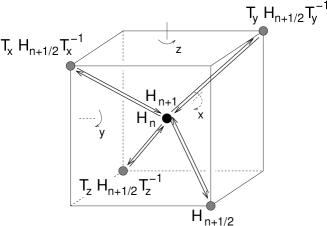
Figure 1: Four SUSY–QM chains for Akulin’s Hamiltonians: thick arrows correspond to SUSY–QM connections. The $180^{\circ}$ rotations about the axes $OX$, $OY$, and $OZ$ correspond to the transformations ${\cal T}_{x}\equiv\hat{R}\sigma_{x}\cdot\bigcirc\cdot\sigma_{x}^{-1}\hat{R}^{-1}$, ${\cal T}_{y}\equiv(i\sigma_{x})\cdot\bigcirc\cdot(i\sigma_{y})^{-1}$, and ${\cal T}_{z}\equiv\hat{R}\sigma_{z}\cdot\bigcirc\cdot\sigma_{z}^{-1}\hat{R}^{-1}$ respectively.

The intertwiners linking eigenstates of $\hat{H}_{n}$ to eigenstates of $\hat{H}_{n+1}$ $(\hat{\Upsilon}_{n+1\,\leftarrow\,n})$, and the intertwiners linking eigenstates of $\hat{H}_{n}$ to eigenstates of $\hat{H}_{n-1}$ $(\hat{\Upsilon}_{n-1\,\leftarrow\,n})$ can be easily extracted from the chain (9): $\hat{\Upsilon}_{n+1\,\leftarrow\,n}=v_{{\cal T}}\left({\cal T}[\hat{B}_{n+1}^{(-)}]{\cal T}[\hat{A}_{n}^{(+)}]\right)$, and $\hat{\Upsilon}_{n-1\,\leftarrow\,n}=v_{{\cal T}}\left({\cal T}[\hat{B}_{n-1}^{(+)}]{\cal T}[\hat{A}_{n}^{(-)}]\right)$, where we fix the arbitrary phase factor $v_{{\cal T}}$ to $v_{{\cal T}}={\cal T}[\hat{\Upsilon}]/\hat{\Upsilon}$, with values $v_{I}=+1$, $v_{x}=-1$, $v_{y}=+1$, and $v_{z}=-1$. Substituting the expressions for $\hat{A}$’s given above, one obtains the following expressions for the intertwiners:

$$\left.\right.\hat{\Upsilon}_{n+1\,\leftarrow\,n}=\partial_{x}-(n+\frac{1}{2})\tanh(x)+\frac{1}{2}(i\sigma_{y})/\cosh(x)$$

$$\left.\right.\hat{\Upsilon}_{n-1\,\leftarrow\,n}=\partial_{x}+(n-\frac{1}{2})\tanh(x)-\frac{1}{2}(i\sigma_{y})/\cosh(x).$$ (22)

Interestingly, while in the intermediate expressions, the intertwiners depend on ${\cal T}$, this dependence disappears in the final expressions (22). Thus, like Hamiltonians $\hat{H}_{n}$, the intertwiners form a one-dimensional representation of the group $\mathrm{Dih}_{2}$.

This (unexplained) property is nontrivial, because the eigenstates of $\hat{H}_{n}$ are doubly-degenerate, and thus, generally, different versions of the intertwiners can target different linear combinations of the eigenstates.

IV Some extensions of the class of reflectionless Hamiltonians

So far, we have shown that Hamiltonians $\hat{H}_{n}=\sigma_{z}\partial_{x}-\sigma_{x}w_{n}(x)$ are reflectionless for $w_{n}(x)=n/\cosh(x)$, for all integer values of $n$. Here, $\sigma_{x,y,z}$ are Pauli matrices. It can be easily shown that the class of reflectionless Hamiltonians can be extended to

$$\hat{H}_{n}(\xi,\,\eta,\,x_{0},\,\phi)=$$

$$\qquad\qquad\sigma_{z}\partial_{x}-\frac{1}{2}(\sigma_{+}w_{n}(x;\,\xi,\,\eta,\,x_{0},\,\phi)+h.c.)$$

$$w_{n}(x;\,\xi,\,\eta,\,x_{0},\,\phi)=\frac{n\xi\exp[i(\eta(x-x_{0})+\phi)]}{\cosh[\xi(x-x_{0})]}\,,$$ (23)

where $\sigma_{+}=\sigma_{x}+i\sigma_{y}$.

V Inverse Scattering Method

The inverse scattering method was developed to solve the initial value problem for integrable nonlinear partial differential equations (NPDE’s). Associated with each integrable NPDE are two linear differential operators, $\hat{L}=\hat{L}(u)$ and $\hat{M}=\hat{M}(u)$, known as the Lax pair. The solution $u(x,t)$ of the NPDE appears as a necessary condition for $\hat{L}$ and $\hat{M}$ to satisfy a Heisenberg-type equation $\dot{\hat{L}}=[\hat{M},\hat{L}]$ Fordy (1994); Drazin and Johnson (1989). Trivially related to $\hat{L}$ is a Hamiltonian $\hat{H}$ that defines a spectral problem $\hat{H}\psi=\lambda\psi$ Ablowitz et al. (1973); Drazin and Johnson (1989). In the case of KdV, $\hat{L}=\hat{H}$. For the sine-Gordon and attractive nonlinear Schrödinger equations, $\hat{L}=\hat{\sigma}_{z}(\hat{H}-\lambda)$. The eigenvector $\psi$ evolves in time through $\hat{M}$.

The procedure for finding $u(x,t)$ is as follows. First, find the scattering data at $t=0$, $S(0)$, for $\hat{H}(u(x,0))$. Next, use the time evolution through $\hat{M}$ to find the scattering data at time $t$, $S(t)$. Lastly, invert the scattering data at time $t$ to find $u(x,t)$. If the $\hat{H}$ operator for a NPDE is reflectionless, then the inversion formula, known as the Gel’fand-Levitan-Marchenko integral equation, greatly simplifies Drazin and Johnson (1989); Fordy (1994), reducing to a system of algebraic equations, and leads to soliton solutions of the NPDE. Thus, finding SUSY–QM chains of reflectionless Hamiltonians becomes a method of generating large families of multi-soliton solutions of the corresponding NPDE.

VI Solitons of the sine-Gordon equation

The sine-Gordon equation is given by

$$\frac{\partial^{2}}{\partial x\partial t}u=\sin(u)\quad,$$

where $u=u(x,t)$, and $x$ and $t$ are light-cone coordinates, related to lab-frame coordinates $\bar{x}$ and $\bar{t}$ by $x=(\bar{x}+\bar{t})/{2}$, $t=(\bar{x}-\bar{t})/{2}$. Direct-scattering for sG is done via:

$$\hat{H}_{SG}=\sigma_{z}\partial_{x}-\sigma_{x}q(x,t=0)\quad,$$ (24)

where $q(x,t)=-u_{x}(x,t)/2$. For $\eta=\phi_{0}=0$, Akulin’s Hamiltonians (23) have this same structure, and they give reflectionless direct-scattering initial conditions for the sine-Gordon equation. Several known solitonic solutions of sG can be identified. In particular, $\hat{H}_{\mp 1}(\xi\geq 0,\,0,\,x_{0},\,0)$ leads to a kink(anti-kink) soliton of initial position $x_{0}$ and velocity $v=(1-\xi^{2})/(1+\xi^{2})$ in the lab frame:

$$u(x,t)=-4\tan^{-1}\bm{\left(}\exp\left\{\mp[\xi(x-x_{0})+t/\xi]\right\}\bm{}\quad.$$

The Hamiltonian $\hat{H}_{\mp 2}(\xi\geq 0,\,0,\,x_{0},\,0)$ leads to a two-soliton solution,

$$u(x,t)=-4\tan^{-1}\bm{\left(}\frac{\mp\sinh\left\{2[\xi(x-x_{0})+t/3\xi]\right\}}{2\cosh\left[-\xi(x-x_{0})+t/3\xi\right]}\bm{}\quad,$$

which consists of two kinks(anti-kinks) that, at $t=0$ collide at $x_{0}$ with velocities $v_{1}=+1/2$ and $v_{2}=-1/2$ in the lab frame (Fig. 2), and that are observed from a reference frame of velocity $V=(3\xi^{2}-1)/(3\xi^{2}+1)$ with respect to the lab frame.

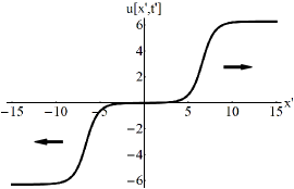
Figure 2: 2-soliton solution of sine-Gordon equation: scattering with Hamiltonian $\hat{H}_{-2}(\xi=1/\sqrt{3},\,0,\,0,\,0)$ leads to a two-soliton solution where two kinks, initially located at the origin, move apart with speeds $v=\pm 1/2$ in the stationary lab frame, shown above. Other values of $\xi$ yield the same solutions but viewed from moving frames.

VII Connection between the SUSY intertwiners and Darboux transformations

At this point, it is instructive to compare the intertwiners (22) to the (well-known) Darboux transformations Sall’ (1982); V. B. Matveev (1991), that also allow the generation of new soliton solutions of nonlinear equations from known solutions. In the context of the sine-Gordon equation, the Darboux connection states, in particular, that for any eigenstate $|\psi(\lambda)\rangle$ of the Hamiltonian $\hat{H}_{SG}$ (24) (parametrized by some $q(x)$) corresponding to an eigenvalue $\lambda$, the state

$$|\tilde{\psi}(\lambda)\rangle=\hat{U}|\psi(\lambda)\rangle$$

is an eigenstate of a new Hamiltonian $\hat{\tilde{H}}_{SG}$ (parametrized by $\tilde{q}(x)$) with the same eigenvalue. The intertwining operator $\hat{U}$ has the form

$$\hat{U}=-\frac{1}{2}\lambda_{0}(\zeta(x)+\frac{1}{\zeta(x)})$$

$$\quad-\frac{1}{2}\lambda_{0}(\zeta(x)-\frac{1}{\zeta(x)})\sigma_{y}+\lambda\sigma_{z}\quad,$$ (25)

and the new field $q$ is

$$\tilde{q}(x)=-q(x,t)+\lambda_{0}(\zeta(x)-1/\zeta(x)))\quad,$$

where $\zeta(x)=(\varphi_{1}(x)+i\varphi_{2}(x))/(\varphi_{1}(x)-i\varphi_{2}(x))$, and $(\varphi_{1}(x),\varphi_{2}(x))^{T}=|\phi(\lambda_{0})\rangle$ forms a “fixed” eigenstate of $\hat{H}_{SG}$ of an eigenvalue $\lambda_{0}$. We conjecture that for any intertwiner $\hat{\Upsilon}$ (22) identified above, there exists a Darboux operator $\hat{U}$ (25), such that $\hat{\Upsilon}$ and $\hat{U}$ coincide on the subspace of the eigenstates of $\hat{H}_{SG}$ of eigenvalue $\lambda$. For example, the choice of $\lambda_{0}=1/2$ and $|\phi(\lambda_{0})\rangle=(\exp[+x/2],\exp[-x/2])^{T}$ leads to the intertwiner $\hat{\Upsilon}_{+1\,\leftarrow\,0}$ (22).

According to our conjecture, our intertwiners do not generate new, previously unknown solutions of the sine-Gordon equation. Nevertheless, the intertwiners (22) allow one to interpret the Darboux links between various Hamiltonians $\hat{H}_{SG}$ (24) as a consequence a hidden SUSY–QM structure. Recall that in the case of the KdV equation (whose analog of $\hat{H}_{SG}$ is the usual stationary linear Schrödinger operator), a similar interpretation is well known Sukumar (1985, 1986); Barclay et al. (1993); Cooper et al. (1988). At the same time, we know of no published work which finds a similarly simple explanation for the existence of Darboux intertwiners (25).

VIII Solitons of the Nonlinear Schrödinger equation

The nonlinear Schrödinger equation with attractive interactions is given by

$$i\frac{\partial}{\partial t}u=-\frac{\partial^{2}}{\partial x^{2}}u-2|u|^{2}u\quad.$$

Direct-scattering is done with

$$\hat{H}_{NLS}=\sigma_{z}\partial_{x}-\frac{1}{2}(\sigma_{+}q(x,t=0)+h.c.)\quad,$$

with $q(x,t)=u(x,t)$. Akulin’s Hamiltonians (23), $\hat{H}_{\pm 1}(\xi>0,\,\eta,\,x_{0},\,\phi)$ produce all one-soliton solutions:

$$u(x,t)=\pm\xi\exp[i(vx^{\prime}/2+\phi)]\,\frac{\exp[it^{\prime}]}{\cosh[x^{\prime}]}\quad,$$

where $v=2\eta$ is the soliton velocity, $x_{0}$ is its initial position, $\phi$ is its phase Drazin and Johnson (1989), $x^{\prime}=\xi(x-vt-x_{0})$, and $t=\xi^{2}t$. In turn, $\hat{H}_{\pm 2}(\xi>0,\,\eta,\,x_{0},\,\phi)$ generates the following breather-like two-soliton solutions:

$$u(x,t)=\pm\xi\exp[i(vx^{\prime}/2+\phi)]$$

$$\qquad\times\frac{4e^{it^{\prime}}\left(\cosh(3x^{\prime})+3e^{8it^{\prime}}\cosh(x^{\prime})\right)}{3\cos(8t^{\prime})+4\cosh(2x^{\prime})+\cosh(4x^{\prime})}\quad,$$

where $v$, $x_{0}$, and $\phi$ now correspond to the velocity, initial position, and the overall phase of the breather, respectively. All $n$-soliton solutions of this type were first obtained, using the inverse scattering method, in Ref. Schrader (1995). Note that in the NLS case, as well as in the sG case, multisoliton solutions can be generated via Darboux transformations Sall’ (1982); V. B. Matveev (1991).

IX The sech-shaped Laser Pulses

Akulin’s Hamiltonians were first studied by Akulin in the context of a two-level, time-dependent system Akulin (2006) that maps to the spatial scattering problem we have considered in this paper: here we present the original problem. Consider a two-level atom subjected to a time-dependent pulse of the form $V_{eg}(t)=V/\cosh\left(t/\tau\right)$ and detuning $\Delta$. Here $V$ is the amplitude of the pulse, $\tau$ is its duration, and $|e\rangle$ and $|g\rangle$ are the excited and ground states, respectively. If we represent the probability amplitudes of the ground and excited states by $\psi_{g}$ and $\psi_{e}$, respectively, the dynamics of the system will obey

$$i\frac{d}{dt}\psi_{g} = +\frac{\Delta}{2}\psi_{g}+\frac{n}{\tau\cosh\left(t/\tau\right)}\psi_{e}$$

$$i\frac{d}{dt}\psi_{e} = +\frac{n}{\tau\cosh\left(t/\tau\right)}\psi_{g}-\frac{\Delta}{2}\psi_{e}\quad.$$

It is known that for specific values of the pulse amplitude, given by $V=n\hbar/\tau$, where $n$ is an integer, the transition probability is zero regardless of the detuning choice $\Delta$ Akulin (2006) (Fig. 3). Mathematically, this property was not well understood. However, a re-interpretation of this problem as finding eigenstates of a reflectionless Akulin’s Hamiltonian $\hat{H}_{n}(\xi=1/\tau,\,0,\,0,\,\pi/2)$ (23) with an eigenvalue $\lambda=-i\Delta/2$ explains the absence of the population transfer in the pulse propagation.

Figure 3: Sech-shaped laser pulse: our SUSY–QM connection of Akulin’s Hamiltonians to the potential-free $\hat{H}_{0}$ also explains a series of specific laser pulse shapes that exhibit a zero ground-excited population transfer for any value of the laser detuning.

X Summary and Outlook

We have shown that Akulin’s Hamiltonians (4) are connected to a potential-free Hamiltonian via supersymmetric chains (9), explaining their reflectionless nature. Akulin’s Hamiltonians lead to multi-soliton solutions when used as direct-scattering initial conditions for the sine-Gordon and attractive nonlinear Schrödinger equations. Additionally, we explain why laser pulses of the form $V(t)=(n\hbar/\tau)/\cosh(t/\tau)$ do not transfer population between the levels of a two-level atom, for any choice of detuning.

The most immediate open question is what specific multi-soliton solutions the $\hat{H}_{n}$’s correspond to for $n>2$ for the sine-Gordon equation. (The soliton solutions generated by $\hat{H}_{n}$ for the nonlinear Schrödinger equation are given in Ref. Schrader (1995).) Additionally, our analysis only contains one free-parameter $\xi$, which is not sufficient to fully classify the known multi-soliton solutions. Additional freedoms may come from different factorization energies leading to other SUSY–QM chains (similar to the analysis in Ref. Sukumar (1986) for the KdV case), and from the inclusion of spatial-shifts to the initial conditions at every step of the SUSY–QM chains.

References

- Kay and Moses (1956) I. Kay and H. E. Moses, J. App. Phys. 27, 1503 (1956).
- Shabat (1992) A. Shabat, Inverse Problems 8, 303 (1992).
- Spiridonov (1992) V. Spiridonov, Phys. Rev. Lett. 69, 398 (1992).
- Witten (1981) E. Witten, Nucl. Phys. B 188, 513 (1981).
- Sukumar (1985) C. V. Sukumar, J. Phys. A 18, 2917 (1985).
- Sukumar (1986) C. V. Sukumar, J. Phys. A 19, 2297 (1986).
- Barclay et al. (1993) D. T. Barclay, R. Dutt, A. Gangopadhyaya, A. Khare, A. Pagnamenta, and U. Sukhatme, Phys. Rev. A 48, 2786 (1993).
- Cooper et al. (1988) F. Cooper, A. Khare, R. Musto, and A. Wipf, Annals of Physics 187, 1 (1988).
- Gardner et al. (1967) C. S. Gardner, J. M. Greene, M. D. Kruskal, and R. M. Miura, Phys. Rev. Lett. 19, 1095 (1967).
- Scott et al. (1973) A. C. Scott, F. Y. F. Chu, and D. W. McLaughlin, Proc. IEEE 61, 1443 (1973).
-
Akulin (2006)
V. M. Akulin,
Coherent Dynamics of Complex Quantum
Systems (Springer, Heidelberg, 2006). - Delone and Krainov (1985) N. Delone and V. Krainov, Atoms in Strong Light Fields (Springer, Heidelberg, 1985).
- Sall’ (1982) M. A. Sall’, Theor. Math. Phys. 53, 1092 (1982).
-
V. B. Matveev (1991)
M. A. S. V. B. Matveev,
Darboux Transformations and
Solitons (Springer, Heidelberg, 1991). - Fordy (1994) A. Fordy, in Harmonic Maps and Integrable Systems, edited by A. Fordy and J. Wood (1994), pp. 7–28.
-
Drazin and Johnson (1989)
P. G. Drazin and
R. S. Johnson,
Solitons: an Introduc-
tion (Cambridge University Press, New York, 1989). - Ablowitz et al. (1973) M. J. Ablowitz, D. J. Kaup, A. C. Newell, and H. Segur, Phys. Rev. Lett. 31, 125 (1973).
- Schrader (1995) D. Schrader, IEEE J. Quantum Electron. 31, 2221 (1995).