Cohomologous Harmonic Cochains 111This is a much shorter incarnation of version 6 of this paper which is available on arXiv as [11].
Abstract
We describe algorithms for finding harmonic cochains, an essential ingredient for solving elliptic partial differential equations using finite element or discrete exterior calculus. Harmonic cochains are also useful in computational topology and computer graphics. We focus on finding harmonic cochains cohomologous to a given cocycle. Amongst other things, this allows for localization near topological features of interest. We derive a weighted least squares method by proving a discrete Hodge-deRham theorem on the isomorphism between the space of harmonic cochains and cohomology. The solution obtained either satisfies the Whitney form finite element exterior calculus equations or the discrete exterior calculus equations for harmonic cochains, depending on the discrete Hodge star used.
Keywords: Finite element exterior calculus; Discrete exterior calculus; Hodge theory; Poisson’s equation; Laplace-deRham operators; Hodge-deRham isomorphism
MSC Classes: 65F10, 68U05, 65N30, 55-04; ACM Classes: F.2.2, G.1.6
1 Introduction
We discuss methods for finding simplicial harmonic cochains – approximations of harmonic forms on simplicial meshes. In particular, we want to find the harmonic cochain cohomologous to a given cocycle. That is, given a cocycle , we want a harmonic cochain such that for some . We either solve an eigenvector problem followed by post processing or use a weighted least squares method.
Harmonic cochains are used in finite element solution of elliptic partial differential equations like the Poisson’s equation . See for instance [2]. They are also useful in computer graphics for design of vector fields, since they can provide a background on which vortices, sources and sinks may be superimposed [9]. In computer graphics they are also useful for finding conformal parameterization for texture mapping and other applications [10].
We prove an easy discrete version of the Hodge-deRham isomorphism theorem. This leads to a weighted least squares based method which is the main contribution of this paper. The linear system is an obvious one and can be derived also from the gradient part of Hodge decomposition or in other ways. The two other methods we describe are based on finding eigenvectors followed by post processing. The least squares method solves the mixed finite element exterior calculus equations for harmonic cochains given in [2, Lemma 3.10]. (This is a result of Demlow and Hirani, and the proof can be found in [11].) For each of the harmonic cochain methods considered, the choice of the Hodge star operator (Whitney or primal-dual) can be made, leading to two variations of each method.
Other methods are those by Gu and Yau [10], and Desbrun et al. [7]. Both of these have some numerical disadvantages especially when Whitney Hodge star is used instead of the diagonal primal-dual Hodge star of discrete exterior calculus. (The Whitney Hodge star is needed for general simplicial meshes, and for the lowest order finite element exterior calculus.) In cases such as 2-dimensional cochains in tetrahedral meshes, the Desbrun et al. method does more work than is necessary for forming the linear system, no matter which Hodge star is used.
2 Preliminaries
Most of the needed background information on algebraic topology and exterior calculus can be found in an earlier longer version of this paper which is still available on arXiv [11]. We use two types of discretizations of exterior calculus – discrete exterior calculus, and finite element exterior calculus. In finite element exterior calculus, we only consider the version that uses Whitney forms.
We first recall the smooth Hodge-deRham theorem on the isomorphism between cohomology and harmonic forms ( or harmonic fields (). (This material is based on [14]). The space of harmonic -dimensional fields on a manifold is denoted . For a closed manifold (i.e., compact manifold without boundary), harmonic forms and harmonic fields are the same, i.e., . However, in the case of compact manifolds with boundary , which we will refer to as -manifolds, one only has that and there can exist harmonic forms which are not harmonic fields [6].
One of the striking properties of harmonic forms or fields is the link they yield between topology and analysis or geometry. For closed manifolds there is an isomorphism between real cohomology and the space of harmonic forms. For compact -manifolds however, even the space of harmonic fields is infinite dimensional due to the possibility of specifying boundary conditions. An isomorphism with cohomology can be obtained by restricting harmonic fields by specifying certain boundary conditions.
The tangential component of a -form is denoted and its value is the value of on the tangential (to ) components of its vector field arguments. Then the normal component of is . See [14, page 27] or [1, page 540]. These can also be defined using the pullback via the inclusion map of the boundary into the manifold. A differential form is said to satisfy the Neumann or absolute boundary conditions if it has zero normal component (), and the Dirichlet or relative boundary conditions if it has zero tangential component (). Let and be harmonic fields satisfying the Neumann or Dirichlet boundary conditions, respectively. Then one has:
Theorem (Hodge-deRham Isomorphism [14]).
If is a closed manifold, then , and if it is a compact -manifold then and .
The space is the (absolute) real -cohomology vector space of , and is the relative real -cohomology vector space of , relative to its boundary. For -manifolds, we will only consider harmonic fields satisfying Neumann conditions. This is because the least squares method is based on a weak form of the Laplace-deRham operator, and in that framework the Neumann conditions are automatic, that is they do not have to be enforced explicitly. For manifold complexes with boundary we will use harmonic cochains synonymously with harmonic Neumann cochains.
3 Eigenvector Methods
Cohomologous harmonic cochains can be computed by first computing a harmonic cochain basis followed by some post processing. Such a basis can be obtained as eigenvectors of the zero eigenvalue of a discrete . The problem of finding eigenvectors can be formulated (in the terminology of finite element methods) using a weak mixed or weak direct method. While nothing is published about the eigenvector method, the weak mixed method was the one used by Arnold et al. [2] in one of their examples.
Let be the smooth Laplace-deRham operator on some manifold . Then the direct eigenvalue problem is to find a nonzero differential form and a real scalar such that . The formal derivation of the weak direct method goes like this: start by posing the problem of finding a such that for all , the inner products being those on forms. Then using the formula for the Laplace-deRham operator, and assuming appropriate boundary conditions (which implies adjointness of and ) this is equivalent to finding a such that for all . If is replaced by its simplicial complex approximation (which we will also refer to as ) then the discretization yields the linear system , where now is the discrete Laplace-deRham operator [11] and is a -cochain. Here is the mass matrix for Whitney -forms or the primal-dual discrete Hodge star. The harmonic cochains are thus the solutions corresponding to the zero eigenvalue for this generalized eigenvalue problem.
For the weak mixed eigenvector method, consider the linear system for the unknowns and :
for all and . Then is a solution if and only if and is a harmonic -form [2, Lemma 3.10]. We discretize these equations and obtain the system matrix
| (1) |
whose eigenvectors corresponding to the zero eigenvalue we seek.
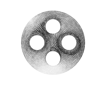
Figure 1 shows results of the eigenvector calculations.The eigenvector methods will often suffice, if all that is needed is some harmonic basis, which may be the common case in finite element exterior calculus. Applications like vector field design in computer graphics may require more control over the process, namely the satisfaction of the cohomology constraint.
|
|
||||
|
3.1 Projection based methods
If a harmonic cochain basis is available, then orthogonal projection to the harmonics can be used to obtain a harmonic cochain cohomologous to a given cocycle . (This method was suggested to us by Ari Stern.) In contrast, the least squares method discussed in Section 4 finds a cohomologous harmonic cochain without requiring any precomputation of a harmonic basis. Moreover, the projection method does not find the potential of the gradient part. If that is needed, then the least squares method equation (4) has to be solved anyway.
Let be a matrix whose columns form a harmonic -cochain basis. Given a nontrivial cocycle , we seek the harmonic cochain such that for some . (Thus we are interested in a Hodge decomposition of . Note that the Hodge decomposition of an arbitrary would be , but since the given is a nontrivial cocycle, it has no curl part.) Since is orthogonal to every column of , we have that for all , where is the that we seek. (The inner product above is the -cochain inner product.) Writing for the vector of unknown coefficients , we can express the last equality as the linear system . After solving this for the unknowns , the vector is the desired . This is the normal equation for a weighted least squares problem (a different system from theh one in Section 4). The matrix of the linear system is of order of the -Betti number and the cost of this projection will be dominated by the matrix vector multiplications needed in forming if the Betti number is small. If the columns of are orthonormal in the inner product then no linear solve is required.
3.2 Pairing with homology basis
For vector field design in computer graphics or in physical applications, the usual cases are dimension 2 with 1-cochains and dimension 3 with 1-cochains or 2-cochains. In the latter case, only solid handles and cavities are relevant since general 3-manifolds are typically not used in such applications. In all these cases, it makes sense to talk of homology basis elements corresponding to topological features. These can be used by pairing with cohomology to find cohomologous harmonic cochains. (This method was suggested to us by Douglas Arnold.) For this one needs an explicit isomorphism , where is the vector space dual of real-valued homology. Note that this method requires not only the entire harmonic cochain basis but also a full homology basis.
Given , define the map by for any . This map is well-defined: given other representatives and , one has . To prove that is an isomorphism, it is enough to show that it is injective. That is, we would like to show that for any , for all implies that . This is equivalent to showing that if is a representative of an element of , for all nontrivial cycles implies that is exact. Since is nontrivial, for some and harmonic cochain . To show is exact is the same as showing . Thus we have to show that given a harmonic cochain , for all nontrivial cycles implies that . We now show this for the case of ( of ) and .
Theorem 1.
Let be a surface simplicial complex. Then is injective (hence an isomorphism).
Proof.
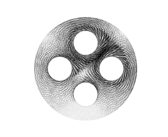
It is enough to consider a homology basis of nontrivial cycles. Suppose has holes and handles. Consider a homology basis corresponding to the holes, handles and tunnels. That is, let be cycles corresponding to of the holes (the remaning one hole is considered the outer boundary), be handle cycles corresponding to the handles, be tunnel cycles corresponding to the handles. (Handle cycles are like longitudes on a torus and tunnel cycles are like latitudes on a torus.) Let be the collection of nontrivial cocycles corresponding to the hole cycles in, and let and be similarly defined. Each such cocycle is a “picket fence” (see Figure 2). Either two edges of a triangle carry a part of or none. The hole cocycles join the boundary of a hole to the outer boundary. The handle and tunnel coycles go around the handle or tunnel. Such cocycles are obtained by dualizing cycles on the dual mesh. By Theorem 2, there is a basis of cohomologous cochains for all , for all , and for all (cohomologous to the corresponding ’s).
Now consider a harmonic 1-cochain that evaluates to 0 on all the basis cycles above. In terms of the harmonic basis above,
| (2) |
Note that evaluates to nonzero on and 0 on every other cycle, evaluates to nonzero on and 0 on every other cycle, evaluates to nonzero on and 0 on every other cycle. , where is the boundary of the corresponding hole since is cohomologous to and is homologous to . But (or whatever value was picked for edges). Likewise, , for since takes value 0 on edges of . Similarly for on other types of cycles, and for the other harmonic basis elements. Thus, the coefficients in (2) are all zero. ∎
If is the closure of a connected open subset of and the topological features of interest are cavities and solid handles then a result similar to the above one can be shown. Now let be a matrix whose columns form a basis of harmonic -cochains and a matrix whose columns form a homology basis corresponding to topological features in the sense described in the proof above. Then contains the harmonic cochains cohomologous to the topological features.
4 Least Squares Method
In what follows, will be a simplicial manifold complex, with or without boundary. All references to are to the discrete Laplace-deRham operators [11]. For a closed manifold, one way to show the Hodge-deRham isomorphism theorem of Section 2 for the smooth case is to use a variational approach [12, Theorem 2.2.1]. One shows that in each cohomology class there is exactly one harmonic form and it is the one with the smallest norm. The norm used is the norm induced from the inner product of differential forms. Inspired by this, we formulate a simple discrete version of this theorem. This is done for harmonic cochains in the case of manifold simplicial complexes without boundary, and for harmonic Neumann cochains in the case with boundary. First we derive the necessary stationarity conditions in the discrete case. For s.t. , we consider the optimization problem , where the is the inner product on -cochains [3]. Writing this in matrix notation, we want to find the minimizer in the optimization problem
| (3) |
From the stationary condition for the minimizer and using properties of the Hodge star matrix, we obtain:
| (4) |
This is the normal equation for the weighted least squares problem . Although the above equation is a necessary condition for solving the optimization problem (3), the matrix may have a nontrivial kernel. In fact in the interesting cases it generally will. (For example, for , the will have dimension equal to the number of connected components in the complex.) Thus, for to be a minimizer we need that the Hessian be at least positive semidefinite, which is true because of the positive definiteness of . In this case, may not be unique, but as we will show next, will be unique. Note that equation (4) is equivalent to which is . This should make the connection to being harmonic more transparent since we also have that .
From the above, if , then it is easy to see that (i) there exists a cochain , not necessarily unique, such that ; (ii) there is a unique cochain satisfying ; and (iii) implies . To see (i) consider the least squares problem . Let be a solution. Some such always exists because least squares problems always have a solution. Note that the norm used in formulating this problem as a residual minimization is the one induced from the Hodge star inner product on cochains. Specifically, the inner product matrix is and the least squares problem minimizes since is the residual. But from properties of least squares [5] the residual is -orthogonal to . Thus we have that since is the adjoint of up to sign in the Hodge star inner product on cochains. In (ii) uniqueness of follows from properties of least squares, and (iii) is obvious since is also closed. Note that unlike in the smooth case, and are adjoints of each other up to sign only. Specifically, for any -cochain and -cochain . From the preceding discussion, we have the following elementary but useful theorem:
Theorem 2 (Discrete Hodge-deRham Isomorphism).
There is a unique harmonic cochain in each cohomology class and it is the one with the smallest norm. Given a cocycle its cohomologous harmonic cochain is where is a solution of .
An alternative derivation of (4) is to project to image of by requiring that for all . Yet another derivation is the following. Given an , to find its Hodge decomposition, one starts with , where we are seeking a harmonic field or cochain and an and . Applying to both sides yields , which is the same as (4) up to sign after the is cancelled from both sides. Note that the linear system for the part is . This has a which cannot be removed by cancellation since this is . In his thesis [4], Bell was motivated by the need to address the inverse Hodge star matrix in order to apply algebraic multigrid to the Hodge decomposition problem. He proposed replacing the Hodge stars by identity and solving the above systems starting with random cochains until one has obtained a cohomology basis. (He did not prove that the procedure is guaranteed to produce such a basis.) He then showed that choosing the basis elements as and solving (4) for each one yields a basis of harmonic cochains. In contrast we have shown above that each such is cohomologous to the corresponding harmonic cochain individually.
|
|
||||||
|
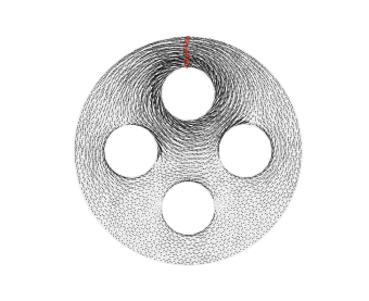

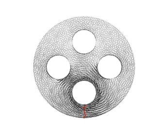
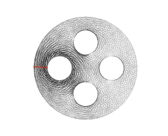
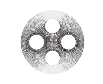
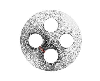
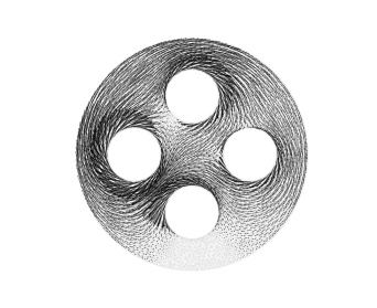
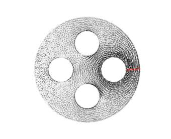
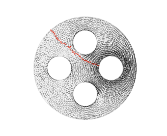
All computations in this paper were done using the Python language with SciPy, NumPy, and PyDEC [3] packages. The top two rows of Figure 2 show the harmonic cochains cohomologous to given nontrivial cocycles on a torus surface. The bottom two rows of Figure 2 show several examples on a planar mesh with holes. To single out a particular hole, so that the harmonic cochain proxy vector field will circulate around that hole, one picks a cocycle connecting that boundary to the outer boundary. Connecting two holes results in a harmonic cochain that circulates about those two holes. For the cochains shown in the third row of Figure 2, from left to right, the values of relative to are approximately , and , respectively. Similarly, for the cochains in the bottom row, from left to right, these values are , and , respectively. Figure 3 shows that the least squares method (as expected) finds the same harmonic cochain when very different initial cocycles from the same cohomology class are given as input. If the cohomologous cochains are denoted , , from left to right, respectively, then the differences between them are , and .
 |
 |
 |
4.1 Linear solvers for the least squares method
As noted earlier, the matrix in (4) is positive semidefinite since will typically have a nontrivial kernel. For example, for for a connected domain, the space of constant functions on the domain is in the kernel of . In this case, it is easy to make the system nonsingular (mod out the nontrivial kernel) by fixing the value at a vertex and adjusting the linear system accordingly. For the case of 2-cochains in tetrahedral meshes however, the kernel of can be large. Let be a three-dimensional manifold simplicial complex. Simple linear algebra and elementary topology reveals that the where is the number of vertices and is the Euler number (the alternating sum of Betti numbers at all dimensions) [13]. For example, for a connected domain with boundary, we will have . By refining the mesh this kernel dimension can be made arbitrarily large. If a direct solver is to be used for solving (4) then one must mod out this potentially large nontrivial kernel. An alternative is to use iterative Krylov solvers as they work well even in the presence of a nontrivial kernel and this is the approach we chose in our experiments. Specifically, we used a conjugate gradient solver without any preconditioning or modifications. Algebraic multigrid is another very efficient alternative whose effectiveness for this problem has been shown in [4].
4.2 Finding the initial nontrivial cochains
In this paper we assume that a nontrivial cocycle is given. Our aim here is not to give algorithms for finding a cocycle. However, a few words about this are in order. An initial nontrivial cocycle in a cohomology class can be found in a number of ways. For surfaces, efficient algorithms to do this exist. By a folklore theorem, in time linear in the number of simplices, one can find a homology basis for the topological dual (e.g., barycentric dual) graph of the triangulation. One can then use Poincaré-Lefschetz duality [13] to get a cohomology basis on the primal mesh. For a boundaryless manifold simplicial complex, one would start with nontrivial cycles on the dual graph. But in case of a manifold with boundary, due to Lefschetz duality, one has to start with a nontrivial relative cycle on the dual mesh, relative to the boundary. One can also start with a random cochain and compute the desired nontrivial cocycle using a Hodge decomposition with standard inner product [4]. Yet another method is to use the persistence algorithm [8]. This is usually implemented using coefficients in finite field and has cubic (in the number of simplices) complexity.
5 Comparisons with Other Methods
The first relevant method to compare with is from the book of Gu and Yau [10] and also appears in their earlier work. The formulation is very simple and straight forward, but it leads to inefficient methods on general simplicial meshes. This method was further simplified by Desbrun et al. [7] who solve a Poisson’s-like equation at a different dimension. The resulting linear systems in both methods suffer from numerical and scalability issues for general simplicial meshes.
Gu and Yau start with a nontrivial cocycle representing a cohomology class in and seek a cochain such that . This leads to the linear system . The presence of the inverse Hodge stars in this systems lead to numerical disadvantages.
Desbrun et al. [7] solve a different Poisson’s equation . A solution to the above equation yields an that is harmonic in the sense of this paper. Of course, if harmonic 1-cochains are being sought, then is a 0-cochain and is the 0 operator. Thus the term is not present. However, the term is superfluous at every dimension as we have shown. Thus their linear system has an extra, unnecessary term. This extra term causes numerical and scalability problems when Whitney Hodge star is used.
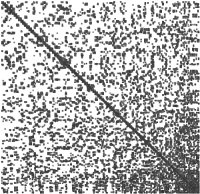
In Figure 4, we compare the sparsity of the least squares and Desbrun et al. matrices for finding harmonic 2-cochains on a tetrahedral mesh of a solid annulus (a solid ball with an internal cavity). The matrices are shown in Figure 4 for both the Whitney and DEC Hodge stars. Both matrices are of the same size but the Desbrun et al. matrix is denser. This is very obvious for the Whitney Hodge star case (14.3 million vs. 56 thousand nonzeros). However, it is also evident in the DEC Hodge star case (94 thousand vs. 40 thousand nonzeros). Here the increased density is due to the extra term in the Desbrun et al. system.
|
The superior sparsity of the linear system matrix in the least squares method leads to improved solution time. To illustrate this, we compare the time taken for again finding harmonic 2-cochains on a tetrahedral mesh of a solid annulus. For the least squares method, using conjugate gradient method (without preconditioning), the times are 0.1355 and 0.1181 seconds for the DEC and Whitney Hodge stars, respectively. For the Desbrun et al. method, these times are 3.510 and 1746 seconds, respectively. We also used a sparse solver in SuperLU for Desbrun et al. system and in this case, the times are 0.3171 and 13.05 seconds, respectively. (All times are averaged over many trials. Also, it may be possible to improve the times for both the methods by using preconditioners or special solvers.) Another least square method is that of Fisher et al. [9]. Comparisons with it are in an earlier version of this paper available on arXiv [11].
6 Conclusions
We presented two methods for finding harmonic cochains in the cohomology class of a given cocycle – an eigenvector method (using direct or mixed formulation) followed by post processing and a least squares method. The most salient feature of the least squares method is in finding a cohomologous harmonic cochain without requiring an entire harmonic or homology basis. The least squares method is numerically superior and independent of the choice of Hodge stars in comparison with the Poisson’s equation methods of Gu and Yao, and Desbrun et al. In future we plan to develop harmonic cochain methods for higher order finite element exterior calculus analogous to the one for Whitney forms. A precise quantification of the efficiency of the least squares method in comparison with the eigenvector method for finding a cohomologous harmonic basis is another direction to pursue.
Acknowledgement
This research was funded in part by NSF Grant DMS-0645604. We thank Douglas Arnold, Alan Demlow, Tamal Dey, Nathan Dunfield, Damrong Guoy, Rich Lehoucq, and Ari Stern for discussions, and Mathieu Desbrun for pointing out the Fisher et al. paper.
References
- [1] Abraham, R., Marsden, J. E., and Ratiu, T. Manifolds, Tensor Analysis, and Applications, second ed. Springer–Verlag, New York, 1988.
- [2] Arnold, D. N., Falk, R. S., and Winther, R. Finite element exterior calculus: from Hodge theory to numerical stability. Bull. Amer. Math. Soc. (N.S.) 47, 2 (2010), 281–354. doi:10.1090/S0273-0979-10-01278-4.
- [3] Bell, N., and Hirani, A. N. PyDEC: Algorithms and software for Discretization of Exterior Calculus, March 2011. arXiv:1103.3076.
- [4] Bell, W. N. Algebraic Multigrid for Discrete Differential Forms. PhD thesis, University of Illinois at Urbana-Champaign, Urbana, Illinois, 2008.
- [5] Björck, A. Numerical methods for least squares problems. Society for Industrial and Applied Mathematics (SIAM), Philadelphia, PA, 1996.
- [6] Cappell, S., DeTurck, D., Gluck, H., and Miller, E. Y. Cohomology of harmonic forms on riemannian manifolds with boundary. arXiv:0508372v1.
- [7] Desbrun, M., Kanso, E., and Tong, Y. Discrete differential forms for computational modeling. In Discrete Differential Geometry, A. I. Bobenko, J. M. Sullivan, P. Schröder, and G. M. Ziegler, Eds., vol. 38 of Oberwolfach Seminars. Birkhäuser Basel, 2008, pp. 287–324. doi:10.1007/978-3-7643-8621-4_16.
- [8] Edelsbrunner, H., Letscher, D., and Zomorodian, A. Topological persistence and simplification. Discrete and Computational Geometry 28, 4 (November 2002), 511–533. doi:10.1007/s00454-002-2885-2.
- [9] Fisher, M., Schröder, P., Desbrun, M., and Hoppe, H. Design of tangent vector fields. ACM Transactions on Graphics 26, 3 (July 2007), 56–1–56–9.
- [10] Gu, X. D., and Yau, S.-T. Computational Conformal Geometry, vol. 3 of Advanced Lectures in Mathematics (ALM). International Press, Somerville, MA, 2008.
- [11] Hirani, A. N., Kalyanaraman, K., Wang, H., and Watts, S. Cohomologous harmonic cochains, 2011. Older longer version (version 6) of this paper. arXiv:1012.2835v6.
- [12] Jost, J. Riemannian Geometry and Geometric Analysis, fourth ed. Universitext. Springer-Verlag, Berlin, 2005. doi:10.1007/3-540-28890-2.
- [13] Munkres, J. R. Elements of Algebraic Topology. Addison–Wesley Publishing Company, Menlo Park, 1984.
- [14] Schwarz, G. Hodge Decomposition—a Method for Solving Boundary Value Problems, vol. 1607 of Lecture Notes in Mathematics. Springer-Verlag, Berlin, 1995.